Towards the Scalability of De- tecting and Correcting Incom-patible Service Interfaces - Mo Diallo June 15, 2020
←
→
Page content transcription
If your browser does not render page correctly, please read the page content below
Bachelor Informatica

Informatica — Universiteit van Amsterdam

                                           Towards the Scalability of De-
                                           tecting and Correcting Incom-
                                           patible Service Interfaces

                                           Mo Diallo

                                           June 15, 2020

                                           Supervisor(s): Benny Åkesson, Jack Sleuters
2
Abstract
    In cyber-physical systems with long lifetimes, updating components is a costly process.
Service-oriented software architectures are used to introduce flexibility into a system. This
allows for modification of the underlying component, which implements a particular version
of an interface, causing the system to evolve. Service interfaces thus create an abstraction
layer over the components. With this abstraction layer, systems can be made up of various
components that may be replaced or modified, provided they implement the same version of
the interface. This abstraction breaks when service interfaces need to be modified, meaning
that all components implementing that interface may fail.
    The Dynamics project proposes a methodology for detecting and correcting incompati-
bilities within service interfaces post-modification. The scalability of the methodology pre-
sented in Dynamics has not been evaluated. They do not have sufficient existing interfaces
to use for evaluations. This thesis aims to provide a starting point for the scalability evalu-
ation of the proposed methodology. This will be done by generating synthetic interfaces of
various complexity. We make two contributions in this thesis. First, we define the notion
of complexity as inputs, outputs and non-determinism. Furthermore, the relation between
these parameters is studied. Second, the methodology for a ComMA interface generator
using user-supplied complexity parameters is introduced.

                                              3
4
Acknowledgements

I would like to express my gratitude to the ESI team at TNO. The time they spent on answering
questions and providing their insights was extremely valuable.
I would furthermore like to thank my supervisor B. Åkesson and J. Sleuters. Their overall help
in meeting with me to discuss the contents of thesis and providing me guidance during writing
were vital.

                                              5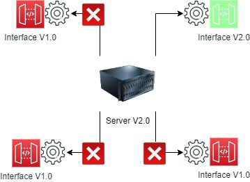
6
Contents

1 Introduction                                                                                                                                                 9

2 Related Work                                                                                                                                                 11

3 Project Background                                                                                                                                           13
  3.1 Dynamics . . . . . . . . . . . . . .             . . . . . .             .   .   .   .   .   .   .   .   .   .   .   .   .   .   .   .   .   .   .   .   13
  3.2 Component Modeling and Analysis                  (ComMA)                 .   .   .   .   .   .   .   .   .   .   .   .   .   .   .   .   .   .   .   .   15
  3.3 Petri nets . . . . . . . . . . . . . .           . . . . . .             .   .   .   .   .   .   .   .   .   .   .   .   .   .   .   .   .   .   .   .   16
  3.4 Portnet Refinement Rules . . . . .               . . . . . .             .   .   .   .   .   .   .   .   .   .   .   .   .   .   .   .   .   .   .   .   17
      3.4.1 Refinement Rules . . . . . .               . . . . . .             .   .   .   .   .   .   .   .   .   .   .   .   .   .   .   .   .   .   .   .   18

4 Synthetic Interface Generation                                                                                                                               23
  4.1 Requirements . . . . . . . . . . . . . . . . .                       .   .   .   .   .   .   .   .   .   .   .   .   .   .   .   .   .   .   .   .   .   23
  4.2 Complexity Parameters . . . . . . . . . . .                          .   .   .   .   .   .   .   .   .   .   .   .   .   .   .   .   .   .   .   .   .   24
      4.2.1 Number of Inputs and Outputs . . .                             .   .   .   .   .   .   .   .   .   .   .   .   .   .   .   .   .   .   .   .   .   24
      4.2.2 Non-Determinism . . . . . . . . . . .                          .   .   .   .   .   .   .   .   .   .   .   .   .   .   .   .   .   .   .   .   .   25
  4.3 Allowed Ruleset . . . . . . . . . . . . . . .                        .   .   .   .   .   .   .   .   .   .   .   .   .   .   .   .   .   .   .   .   .   25
      4.3.1 Definition . . . . . . . . . . . . . . .                       .   .   .   .   .   .   .   .   .   .   .   .   .   .   .   .   .   .   .   .   .   25
      4.3.2 Rules for Refinement Applications .                            .   .   .   .   .   .   .   .   .   .   .   .   .   .   .   .   .   .   .   .   .   26
  4.4 Generation Scheme . . . . . . . . . . . . .                          .   .   .   .   .   .   .   .   .   .   .   .   .   .   .   .   .   .   .   .   .   28
      4.4.1 Applying Parameters to Generation                              .   .   .   .   .   .   .   .   .   .   .   .   .   .   .   .   .   .   .   .   .   29
      4.4.2 Generational Description . . . . . .                           .   .   .   .   .   .   .   .   .   .   .   .   .   .   .   .   .   .   .   .   .   29
  4.5 Evaluating Non-Determinism . . . . . . . .                           .   .   .   .   .   .   .   .   .   .   .   .   .   .   .   .   .   .   .   .   .   30
  4.6 Limitations . . . . . . . . . . . . . . . . . .                      .   .   .   .   .   .   .   .   .   .   .   .   .   .   .   .   .   .   .   .   .   32
      4.6.1 Generational Scope . . . . . . . . . .                         .   .   .   .   .   .   .   .   .   .   .   .   .   .   .   .   .   .   .   .   .   32
      4.6.2 Randomized Complexity Generation                               .   .   .   .   .   .   .   .   .   .   .   .   .   .   .   .   .   .   .   .   .   33

5 Converting Internal Representation                                                                                                                           35
  5.1 Internal Representation . . . . . . . . . . . . . . . . . . . . . . . . . . . . . . . .                                                                  35
  5.2 Conversion of Internal Representation . . . . . . . . . . . . . . . . . . . . . . . .                                                                    35

6 Experiments                                                                                                                                                  39
  6.1 Maximum Prevalence of Non-Determinism . . . . . . . . . . . . . . . . . . . . . .                                                                        39
  6.2 Relation Input/Outputs to Prevalence . . . . . . . . . . . . . . . . . . . . . . . .                                                                     41

7 Conclusion                                                                                                                                                   43
  7.1 Future Work . . . . . . . .      .   .   .   .   .   .   .   .   .   .   .   .   .   .   .   .   .   .   .   .   .   .   .   .   .   .   .   .   .   .   43
      7.1.1 Scalability Analysis       .   .   .   .   .   .   .   .   .   .   .   .   .   .   .   .   .   .   .   .   .   .   .   .   .   .   .   .   .   .   44
      7.1.2 Modifying Ruleset .        .   .   .   .   .   .   .   .   .   .   .   .   .   .   .   .   .   .   .   .   .   .   .   .   .   .   .   .   .   .   44
      7.1.3 Complexity . . . . .       .   .   .   .   .   .   .   .   .   .   .   .   .   .   .   .   .   .   .   .   .   .   .   .   .   .   .   .   .   .   44
  7.2 Ethics . . . . . . . . . . . .   .   .   .   .   .   .   .   .   .   .   .   .   .   .   .   .   .   .   .   .   .   .   .   .   .   .   .   .   .   .   44

                                                           7
A Experiment Datapoints 49
A.1 6.1 Experiment 1 . . . . . . . . . . . . . . . . . . . . . . . . . . . . . . . . . . . 50
A.2 6.1 Experiment 2 . . . . . . . . . . . . . . . . . . . . . . . . . . . . . . . . . . . 51
B Example Interfaces and Conversions 53
B.1 Example 1 . . . . . . . . . . . . . . . . . . . . . . . . . . . . . . . . . . . . . . . . 53
B.2 Example 2 . . . . . . . . . . . . . . . . . . . . . . . . . . . . . . . . . . . . . . . . 55
B.3 Example 3 . . . . . . . . . . . . . . . . . . . . . . . . . . . . . . . . . . . . . . . . 57
8CHAPTER 1
Introduction
Technological needs are ever changing. Whether that is due to regulation, business needs, or
technological advancements; systems will regularly need to be updated to comply with these new
requirements. Within the context of these ever changing systems, issues unfold, such as in cyber-
physical systems. In cyber-physical systems with long lifetimes, it is infeasible to continuously
update individual components to adhere to new requirements or technological advancements.
One method of facilitating component updates is through the implementation of service-
oriented software architectures. By using service interfaces, an abstraction layer over the service’s
components is created. This abstraction layer makes it possible for components of the system to
be replaced by other components implementing the same interface. If this component implements
the same version of the interface, even if the implementation of the component or the underlying
technology differ, it will remain compatible with the system.
Utilizing services interfaces makes a system resistant to changes within the individual com-
ponent. This highlights one issue, the service interface itself may eventually need to be updated.
Figure 1.1 shows an example of such a scenario. Assuming all implemented interfaces were pre-
viously version 1, the example shows that the server and one component have been manually
updated to version 2. The three other components implement the original version of the in-
terface. This shows that when a service interface is updated, all server and client components
implementing the old interface may fail. Manually updating these components is expensive and
time consuming.
In collaboration with Thales, ESI (TNO) has developed an initial approach to detect in-
compatibilities between different versions of interfaces. Furthermore, their approach attempts
to correct incompatibilities through adapter generation. The methodology is presented in the
Dynamics [1] project. The proposed solution, which introduces a five-step methodology for the
detection and correction of incompatibilities, requires a scalability analysis of this approach in
the context of the required use case. The work conducted in this thesis provides a starting point
towards evaluating the scalability of this approach. This will be done by generating complex
interfaces. The findings from this thesis may be used in future work to establish the boundaries
of the proposed methodology.
Figure 1.1: Update to service interface requires manually updating components.
9Figure 1.2: Context of thesis within the Dynamics project.
This thesis consists of three contributions, Figure 1.2 shows our contributions within the
greater context.
1. We introduce and define the concept of complexity in synthetically generated interfaces as
the number of inputs, outputs and the amount of non-determinism. The relation between
the parameters is evaluated theoretically and experimentally.
2. A methodology for the synthetic generation of portnets, a subset of Petri Nets, using
user-defined complexity parameters is presented. This utilizes previous research [2] on
refinement rules for portnets. The application and properties of these rules is studied to
devise a methodology for applying them in a synthetic generational context.
3. The methodology for portnet generation is extended by introducing a converter to a
ComMA interface specification.
The rest of this thesis is structured as follows. Chapter 3 introduces the background this thesis
builds upon. Chapter 4 introduces the methodology for generating synthetic interfaces of various
complexity. This is done by defining the complexity parameters and introducing the generation
scheme. In the following Chapter 5, the conversion process of a generated portnet to a ComMA
interface is described. The generated methodology is evaluated in Chapter 6 by performing
experiments and elaborating on the results. Chapter 7 will elaborate on the conclusions of this
thesis.
10CHAPTER 2
Related Work
There are a multitude of studies that focus on the synthetic generation of models for various types
of analysis. “Task Graphs for Free” [6] introduces the generation of task graphs represented as
directed acyclic graphs. The problem solved in the paper aims to assist researchers in re-creating
examples by ensuring that there is a one-to-one relation when providing the same parameters to
their proposed generator.
“SDF For Free” [14] provides a similar approach. User-supplied parameters are provided to a
generator to create Synchronous DataFlow Graphs.
Both these papers align with the intent of this thesis: synthetically generating a model to perform
various evaluations. In the context of our work, this is to facilitate scalability evaluations.
Where they differ is that they do not directly specify which parameters influence the result of
the generator. It is not intuitive how the chosen parameters correspond to the output of the
generation, and thus the usage of their methodology already requires a substantial amount of
knowledge in the topic.
In contrast to the previous papers, this generator aims to provide users with intuitive pa-
rameters that directly affect what is generated. Furthermore, these parameters are also directly
responsible for adding complexity within the generated interface, allowing one to argue between
the complexity of two different interfaces utilizing only the given parameters.
Furthermore, the result of the generator that we devise will be completely random. The same
parameter values may result in completely different structures.
1112
CHAPTER 3

                                                    Project Background

The goal of our work is to generate part of the required tooling for complexity analysis of the
work conducted in Dynamics [1]. We generate the original ComMA model, as seen in Figure 3.1.
This chapter introduces the various background concepts this project builds upon. In Section
3.1 the Dynamics project, for which this work is conducted, is introduced. In Section 3.2 we
present one of the key concepts of the Dynamics project, ComMA interface specification. This
is further extended in Section 3.3 by the introduction of Petri Nets. Finally, the focus of this
generator, portnets and their refinement rules, are presented in Section 3.4.

3.1 Dynamics
The Dynamics [1] project provides a solution to the problem of “complex systems that need to
continuously evolve”.
The contributions made in the Dynamics project result in the five-step methodology for the
detection and correction of service interface incompatibilities.

                  Figure 3.1: Five-step methodology proposed by ESI (TNO)

   The five-step methodology for detecting and correcting incompatible service interfaces is
shown in figure 3.1. A brief summarized version of the explanation of each step is as follows:
  1. The first step within the proposed solution uses research done previously with Philips [8].
     The essence of the research defines modeling interface behavior and structure using ComMA
     (Component Modeling and Analysis) framework.
  2. In the second step, from the earlier created ComMA models an Open Net (Petri Net) [11]
     is generated.
  3. From the third step, detection and correction happens. This starts with accordance check-
     ing [10] using the tool Fiona [12]. If these two interfaces are in accordance, all clients of
     the old interface are compatible with the updated interface. Two different interfaces do
     not have to be incompatible. For example, one could have two different interfaces where

                                               13
the updated one includes an optional feature. These two interfaces would then still be in
accordance.
In contrast, if for example a new mandatory signal is added, they will not be in accordance
and clients will no longer work properly.
4. If during step three the two interfaces were found not to be in accordance, what remains
is the generation of a corresponding adapter. This is described in the proposed solution as
an approach based on controller synthesis [7].
5. As final step, if an adapter can be generated, the corresponding C++ code for the INAET-
ICS architecture [4] is generated.
143.2 Component Modeling and Analysis (ComMA)
ComMA [8] is an approach utilized for interface specification. The problem statement described
in the paper discusses that interfaces are often only described by their signature. They go on to
state that timing and data constraints usually stay implicit. The paper introduces an approach
that avoids these problems by formalizing interface specifications.
ComMA is described as a state machine-based DSL. The framework supports interface speci-
fication through providing an interface structure, interface behavior and data/timing constraints.
Furthermore, ComMA provides the ability to monitor the interface behavior during execution.
This way it can be checked that a system conforms to the interface specification.
In our work we will focus on how interface behavior is specified with ComMA.
Listing 3.1: Simple ComMA light switch example
1
2 machine LightSwitch {
3 initial state OFF {
4 transition trigger: LSOn
5 next state: ACK_ON
6 }
7
8 state ACK_ON {
9 transition
10 do:
11 LTAck
12 next state: ON
13 }
14
15 state ON {
16 transition trigger: LTOff
17 next state: OFF
18
19 }
20 }
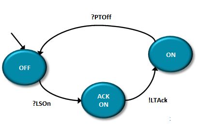
ComMA represents interface behavior as a traditional state machine. Listing 3.1 shows a simple
example of a light switch interface. Of importance within the context of our work are the basics:
signals, notifications, transitions and states. Signals are client to server communication and
notifications are server to client communication.
The provided example assumes a server-sided viewpoint for a remote-controlled light switch.
When the light switch is in the OFF state, upon receiving the signal LSOn, it goes into
the ACK_ON state. Within this state an acknowledgement follows by sending the LTAck
notification. The server will after these actions be in the ON state. Eventually, the client can
choose to switch the light off again by sending LTOff, which results in the server going back to
the OFF state. Figure 3.2 shows the corresponding communicating finite-state machine [5], “?”
denotes an incoming signal, while “!” denotes an outgoing notification.
Figure 3.2: Communicating finite-state machine representation of a light switch.
153.3 Petri nets
Petri Nets, or place/transitions nets, are a particular kind of directed graphs utilized for the
modelling of distributed systems [13]. Using the terminology of graphs, a Petri Net can be
considered as having two different types of nodes, places and transitions. The directed edges
within graphs are referred to as arcs. How this can be visualized is shown in Figure 3.3.
When modelling systems using Petri Nets, places can be considered as conditions. The truth
value of these conditions are considered markings. The marking of a place p, Mp , is a natural
number representing the tokens in that place. Referring back to the modeling example, a place
with three markings can be said to have fulfilled three of its pre-conditions.
Transitions within Petri Nets can be considered as events. These transitions have a number
of input places and output places, connected by arcs between them. The firing (activation) of a
transition is dependent on it being enabled. An enabled transition requires all connected input
places to contain a token. The example in Figure 3.3 shows tokens only in the places labeled as
“Input” and “Initial Place”. Therefore, the first transition is enabled, while the second transition
is disabled. When a transition is fired, it consumes one token from all of its input places and
produces a token in all the output places. Therefore, in the given example the firing of transition
1 would produce a token in place P 2.
Figure 3.3: Terminology of Petri Nets
Petri Nets are used within the Dynamics [1] project to detect incompatibilities. There are
three primary reasons stated within the paper. The first reason is due to it being possible to
translate interfaces specified in ComMA to a Petri Net. The second reason is due to Petri Nets
supporting the modeling of synchronous and asynchronous communication. The final reason is
due to already existing analysis methods for detecting and correction of incompatibilities [16].
163.4 Portnet Refinement Rules
This background section covers the refinement rules introduced in [2]. We introduce the concept
of portnets, a special case of workflow nets [15] [17]. In the context of this work, it is not integral
to know what workflow nets are, hence this explanation will be omitted.
There are several properties that valid portnets must adhere to. First, we introduce the
concept of markings: each portnet consists of a single initial marking Pinitial for which goes that
no arc in the net directs to it. Therefore, given an arc as the tuple < aorigin , adestination > then
{a : adestination == Pinitial } = ∅. Furthermore, a portnet must have a final marking, meaning a
place with no outgoing arcs, formally: {a : aorigin == Pinitial } = ∅. We now come towards weak
termination. In [2] the concept of weak termination is introduced. In Figure 3.4 a valid portnet is
given that weakly terminates. The paper states the definition as “The weak termination property
states that in each reachable state of the system, the system always has the possibility to reach
a final state”.
Using the portnet, that means that from any place, the system will reach the final marking.
Consequently, all tokens within the portnet will be in the final marking.
Figure 3.4: Valid weakly-terminating portnet
Another concern within portnets is the choice property. The property states that for any given
place, all transitions directly following that place must have the same direction of communication.
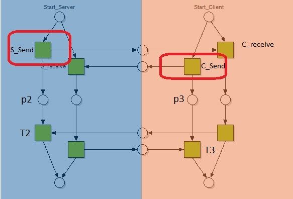
Figure 3.5 shows an example in which this does not happen.
Figure 3.5: Mirrored client example of choice property violation.
17If both the client and server decide to send, in CSend and SSend respectively, a deadlock
occurs. The transitions directly following, T 2 and T 3, are receive for both the client and server.
Consequently, neither the client nor server can ever reach the final marking.
To continue, portnets must also satisfy the leg property. The leg property refers to the
conditions each leg in the portnet must satisfy. A leg is defined as being a path within the
portnet that deviates from another path by a split and is concluded by a join. Furthermore, the
existence of a single path from the initial place to the final marking is also considered as being a
separate leg. The leg property requires each path to have at least two transitions in alternating
direction: an input and output. Therefore, each leg must have one transition that is an input
and one that is an output.
The example in Figure 3.6 shows a portnet that violates the leg property.
Figure 3.6: Mirrored client example of leg property violation.
The figure shows that the portnet is not weakly terminating: there are still remaining tokens
even though the final places have been reached for both the client and server. To understand
how this occurs we refer to the server side of the example. In the beginning, a token exists at
S_Start which is consumed to generate one token in S_P 2. From there it is possible for the
transition S_T 2 to be triggered as it contains a token in its only input place, S_P 2. This will
generate a token in S_P 3 and SC1. This is where the issue starts, when S_T 3 is triggered it
consumes the token in S_P 3 and produces a token in S_P 2. This process may now repeat itself
any number of times, causing the token count in SC1 to increase. Note how both the client and
server can in C_P 2 and S_P 2 continue to the final places without ever having to consume the
generated tokens. Therefore, this example does not weakly terminate: it contains leftover tokens
upon reaching the final places.
The final property we introduce covers transitions. The property states that for a portnet to be
valid, all of its transitions must connect to exactly one interface place and one input or output
place.
3.4.1 Refinement Rules
The base of synthetic interface generation is formed around a construction method [2], which
uses five different refinement rules that derive a Petri Net through continuous rule application.
With exception of the fifth rule, each of these rules can be split into base rules and modified rules.
18The base rules are the starting point for refinement, they operate upon a transition or place and
generate a new structure within the portnet. The modified rules can be best described as altering
the generated net to adhere to the validity properties of portnets, adding inputs/outputs and
ensuring the leg and choice property are complied with.
This section studies the aforementioned rules, such that an appropriate way to apply them
can be devised. These rules will be essential to creating valid portnets while adhering to user
supplied complexity parameters.
There are five refinement rules that are to be considered and their explanation will be given in
the following subsections.
R0: Default Place Refinement
The default rule, R0, forms the base of the refinement rules. As seen in Figure 3.7, the base
rule converts a single place into a structure of P lace → T ransition → P lace. The modified
rules alter this construct by adding either a single input or output to the transition. It should
be noted that the modified rules of R0 are the only rules that may generate a single input or
output. All other refinement rules add an equal number of inputs and outputs.
Figure 3.7: R0 adds a single place and transition, its modified rules generate one input and
output
R1: Transition Refinement
The transition refinement rule, R1, provides an expansion of a transition, Figure 3.8 shows this.
In expanding a transition, it adds one additional place and transition. An important characteris-
tic that presents itself can be seen when the modified rules are applied. The transition expansion
is considered as being part of a leg. As discussed earlier, the leg property states that within
every leg, there must be at least two transitions with different directions of communication. The
two modified rules satisfy this condition by adding one input and output to the two transitions.
The only difference between the two modified rules is the order in which this is done.
Figure 3.8: R1 adds a single place and two transitions, its modified rules generate one input and
output.
19R2: Non-deterministic Transition Refinement
The non-deterministic transition refinement rule, R2, is one of the rules that controls the non-
determinism of the generated net. Like rule R1, it is a transition refinement rule. The difference
between these rules lies in how they refine the transition. R2 duplicates a transition by adding
another transition with the same start and end, as can be seen from Figure 3.9. The issue with
the base rule of R2 is that it generates a structure which violates the leg property. To account for
this, these legs need to be expanded, which can be seen as applying the base rule of R1 upon both
generated transitions. When this is not done correctly an invalid portnet will be generated. This
occurs when two different modified versions of R1 would be applied to add the inputs/outputs.
This would violate the choice property, which requires all transitions directly following the place
(having an incoming arc from it) to have communication in the same direction. The modified
rules fix this issue by adding an additional place and transition in each leg. To preserve the
choice property, the order of inputs and outputs in each leg is the same.
Figure 3.9: R2 adds one place and transition. The modified rules add two transitions and places.
Furthermore, the modified rules add two inputs and outputs.
R3: Cyclic Place Refinement
Thus far, all rules have resulted in a structure where places and transitions are sequential. There
are no loops and consequently there is no way to go back to any previous place within the net.
Rule R3 (Figure 3.10) changes that by introducing a cyclic structure from a place refinement.
20Figure 3.10: R3 adds one transition. The modified rules add an additional place and transition.
Furthermore, one input and output are added.
The base rule of R3 introduces a structure that violates the leg property. The resulting
P 1− > T ransition− > P 1 structure does not have at least two transitions which have different
directions of communication. Thus, to account for this property the modified rules add an extra
transition and ensure both transitions have alternating directions of communication.
An important thing to note is that R3 similarly to R2 introduces non-deterministic behavior.
This is dependent on the place which it is refined upon. Figure 3.11 shows an example of
how R3 may be applied upon P2 to introduce non-determinism. When R3 is applied upon a
non-deterministic place, the already existing outgoing arc becomes non-deterministic. Thus, the
application of R3 would introduce 2 non-deterministic arcs to the net. However, if another appli-
cation of R3 follows upon that same place (P 2), this would only introduce one non-deterministic
arc into the net.
Figure 3.11: Introducing non-deterministic behavior by applying rule R3 upon place P 2.
R4: Concurrent Place/Transition Refinement
Rule four provides a special case within construction. Unlike the other rules thus far, R4 is not
extended by additional modified rules introducing inputs or outputs. As seen in Figure 3.12, this
rule only adds add concurrency to an initial construct of T ransition → P lace → T ransition.
21Figure 3.12: R3 adds one transition. The modified rules add an additional place and transition.
Furthermore, one input and output are added.
In the context of the Dynamics project, this rule is not supported. This rule introduces
concurrency, which means the resulting structure cannot be represented as a state machine.
This construct is thus not a portnet and is also not supported in ComMA, as ComMA interfaces
are state machines [8]. Considering the project pipeline as per Figure 3.1, this rule does not
introduce any constructs that could be a result of the proposed solution. For this reason, the
generator will not include this rule by default.
22CHAPTER 4
Synthetic Interface Generation
This chapter discusses the synthetic generation of interfaces of varying complexity. This chapter
is split into six sections. Section 4.1 will discuss the essential requirements the generator must
satisfy. Section 4.2 introduces and defines the complexity parameters. The allowed ruleset is pre-
sented in Section 4.3. This allowed ruleset is used in Section 4.5 and 4.4 to discuss parameterized
generation and devise the generation scheme for portnets adhering to user supplied complexity
parameters. This chapter concludes with Section 4.6 discussing the limitations of the portnet
generator.
4.1 Requirements
The requirements imposed on the generator are motivated by the work conducted in Dynamics [1].
This is done by performing accordance checking, and adapter generation if necessary. The
proposed solution by Dynamics solves the issues of having to update all components implementing
an interface, post-modification of this interface.
The goal of this thesis is to develop a generator capable of creating interfaces that emulate
the properties of those supplied to Dynamics. These generated interfaces can then be used for
testing the solution and for conducting a scalability analysis of the methodology proposed by the
Dynamics project.
There are various requirements that the generator must satisfy. Before making the requirements
concrete, it should be made clear where in the Dynamics pipeline (Figure 3.1) the generator
operates: this will define what the output of the generator is. Figures 4.2 and 4.1 show the two
possible approaches to generation.
Figure 4.1: Option 1: generating Open (Petri) Nets.
23Figure 4.2: Option 2: generating ComMA models.
The first approach is to generate portnets. This is the input accepted by FIONA to enable
accordance checking and adapter generation.
The second approach is to generate ComMA interfaces. The Dynamics project provides a con-
verter, which would then translate this into a portnet. Subsequently, the portnet would be
provided to FIONA as input.
The biggest shortcoming to the first approach is that it assumes the converter is fixed. If this
were not the case, and the converter is later modified, resulting in an elimination or addition of
possibilities, this thesis’s generator would be outdated, and it could no longer accurately be used
for scalability analysis.
As our goal is to synthetically generate interfaces, which can later be utilized for scalability
analysis, the generator should solely consider interfaces that can be a result of Steps 1 and 2 in
the proposed five-step methodology. If the first approach was chosen, we would need to evaluate
how the converter makes a portnet out of a ComMA model. This so that the generator does not
produce any interfaces that could not be created by the converter.
This gives the motivation behind the choice for the second approach: by generating ComMA
models, one makes the generator more resistant to changes within the Dynamics project.
With the knowledge of what is to be generated, the requirements can now be formalized.
1. The first requirement is that a notion of complexity must be defined. The generator
needs to be able to generate interfaces of various complexity. Henceforth, it is essential
that what is considered as complex can also be passed to the generator as parameters.
These parameters can be used during scalability analysis to get an understanding of which
constructs within the generated portnet add the most complexity to either accordance
checking and/or adapter generation.
2. The second requirement is that the generator must produce valid portnets. A converter
should be included alongside the generator to convert the generated portnets into ComMA
interface specification.
3. As scalability analysis requires two ComMA interfaces, an old and new interface, the gen-
erator should provide a format which allows further extensions of the generator to perform
modifications upon the constructed interfaces.
4.2 Complexity Parameters
Synthetic interface generation concerns itself with generating interfaces of various complexity.
Thus far, the notion of complexity has not been defined. This section will introduce three non-
zero parameters the generator considers as adding complexity: inputs, outputs and the prevalence
of non-determinism. Furthermore, this section will concern itself only with explaining and defin-
ing these parameters. Parameter constraints and how generation takes them into account is left
for Section 4.5.
4.2.1 Number of Inputs and Outputs
Out of the three parameters, inputs and outputs are the most trivial. In the case of ComMA
interfaces, inputs and outputs translate to signals and notifications, respectively. Defined in the
24requirements, the decision was made to generate portnets which are then converted to ComMA
interfaces. As mentioned in Section 3.4, one of the requirements of portnets is that every tran-
sition is connected to one input or output. Thus, the number of inputs and outputs directly
relate to the number of transitions in the net. Therefore, as transitions dictate the number of
places present, indirectly the number of inputs and outputs specified are a way of controlling the
size of the generated portnet. Parameters are specified as integers to the generator in the range
inputs, outputs > 0.
4.2.2 Non-Determinism
The third controllable parameter during generation is that of non-determinism. Compared to
inputs and outputs, non-determinism is of more interest, as the definition is open to various
interpretations.
Definition
The definition of the prevalence of non-determinism is given as the percentage of arcs in the
generated net which originate from a state with multiple outgoing arcs. Formally:
a =< aorigin , adestination > 2-tuple representation of arc (4.1)
Ap = {a : aorigin == p} Arcs (a) originating from place P (4.2)
N = {p : |Ap | > 1} Non-deterministic places (4.3)
X = {a : aorigin ∈ N } Arcs with origin in non-deterministic place (4.4)
|X|
prevalence = Prevalence of non-determinism (4.5)
total arcs
What the equations show is that an arc is a 2-tuple where the elements are the originating
and destination place, respectively. The set of arcs originating from a place, p, is denoted by
Ap . A place within a portnet is said to belong to the set of non-deterministic places, N , if the
cardinality of Ap is greater than one, meaning multiple outgoing arcs. Furthermore, all arcs that
are non-deterministic have their origin as element of the set N .
The definition of the prevalence of non-determinism follows as the fraction of non-deterministic
arcs outgoing from places in the entire portnet.
4.3 Allowed Ruleset
Thus far, this chapter gave the requirements that interface generation must adhere to. Further-
more, the complexity parameters have been introduced and defined. This section will build on
the introduced topics to devise a generation scheme utilizing the portnet refinement rules from
Section 3.4. The paper [2] introducing these rules introduces the concept of weak termination:
“From each reachable state, the system has the option to eventually terminate.”
In this section, these rules are used to generate the allowed ruleset: the set of rules which may
be subsequently followed by another rule to generate valid portnets.
The allowed ruleset guarantees that using the construction rules in the way described retains
the properties of portnets, as given in Section 3.4. Furthermore, facilitates the creation of a
refinement scheme using the described complexity parameters introduced in Section 4.2.
4.3.1 Definition
The paper that describes the refinement rules does not directly provide information for adopting
these rules in a generative way. Furthermore, the paper only concerns itself with the validity of
the portnet itself. The notion of complexity does not appear within the paper. Therefore, as our
generator needs consider the user-supplied parameters, we introduce a refinement scheme which
extends these rules for usage in the context of this thesis. A state machine representation is
given in Figure 4.3, this is used in the following subsections to elaborate on the rules concerning
25application of the construction rules. Final states are modified rules denoted by two circles; they
indicate the end of a refinement iteration.
R1′
R0′ R1 R4
R0
R0” R1”
ST ART
R3 R3′ R2 R2′
R3” R2”
Figure 4.3: Ruleset as a state-machine showing the allowed order of rule applications.
Refinement Iteration
The application of the refinement rules is done within refinement iterations. A refinement it-
eration is a sequence of refinement rules applied on an existing place, while preserving portnet
properties. To further elaborate, each refinement iteration starts with a single place. on this
place, one may according to the allowed ruleset apply a single rule (R3 or R0). From this point
forward, the allowed ruleset is in a new state depending on the rule applied. A refinement
iteration proceeds by randomly selecting rules based on the rule that was previously applied.
This continues until a final state is reached. This random selection is done while adhering to
the selected parameters, and taking into account that the properties of a valid portnet must be
retained after a full refinement iteration.
Once a final state is reached, the refinement iteration concludes, and the resulting structure is
guaranteed to be a valid portnet. This portnet then provides the basis of subsequent refinement
iterations. This continues until the stop conditions, the supplied parameter values, are reached.
4.3.2 Rules for Refinement Applications
Within refinements, the generator distinguishes between two refinement patterns: meaning a rule
is either a place or transition refinement. A refinement iteration is composed of refinement rules
that replace/expand the selected part of the portnet. Only base rules are considered as being
part of a refinement pattern, meaning that only they refine a transition or place. Modification
rules solely serve to ensure the result of a refinement iteration is a valid portnet. Therefore,
when evaluating the refinement rules, the only rules that perform place refinement are the base
rules R0 and R3. The three other base rules perform transition refinement. Thus, excluding
iterations that include applications of R4 (excluded in this work), all refinement iterations start
with exactly one place refinement optionally followed by a transition refinement. The refinement
iteration is then concluded by applying a modified rule.
Start
The start state marks the beginning of a refinement iteration. Each refinement iteration starts by
randomly selecting one of the places within the portnet. From here on, the refinement iteration
starts at random, either R0 or R3 is selected for further refinement of the portnet. As per the
26properties of portnets, each portnet must have one initial place and one final place. Due to
this restriction, R3 is excluded from being applied on these places. Thus, the first
refinement iteration, during which the portnet only consists of one single place, may
not start with R3. Furthermore, R3 is also excluded from being applied on the final place.
The final place may change during refinement iterations; hence the generator keeps track of this
and appropriately labels the final place while refinement occurs.
Rule R0
Within the allowed ruleset, if selected, the R0 state marks the first rule within a refinement
iteration. This rule, as introduced earlier, refines a single place and the result is a P lace →
T ransition → P lace. However, this is not a valid construct. The transition must meet one
condition to guarantee that the portnet is valid: it must be connected to an input or output.
The only way to satisfy this condition is by either applying modified rules on the transition,
or refining the transition further, ensuring that this property is satisfied later. The places that
have been introduced during the refinement need not be considered. These places can further be
refined in subsequent iterations, as opposed to transitions which must be closed (having a single
input/output connected) to comply with the properties of portnets. What follows is that from
R0, the only further rules that may be applied are modified rules or the transition refinement
rules, R1 and R2.
Rule R3
The cyclic place refinement rule, R3, has two restrictions. As mentioned earlier, it may not be
applied on the places denoted by start or final. This means that it may only be applied on
intermediate places. This introduces an interesting construct given in Figure 4.4.
Figure 4.4: Possible choice property violation.
Observing this figure, one can note that R3 generates non-deterministic behavior. Further-
more, in the example given, if t1 was to have an input connected to it: the choice property would
have been violated as not all transitions following P2 have the same direction of communication.
Fortunately, R3 introduces an equal number of inputs and outputs regardless of what modified
rule is applied. Thus, if an application of the modified rule of R3 would result in a choice prop-
erty violation, this is replaced by the application of the other modified rule.
An interesting property of the modified rule of R3 is that it is an application of the base rule R1
and a modified version of R1, on the transition resulting from the application of R3.
Rule R1 and R4
R1 is always preceded by an application of the default rule, R0. The base rule of R1, which creates
a T ransition → P lace → T ransition construct must always be followed by an application of a
modified rule of R1 to reach a final state. This is due to the leg property, in the case of R1 there
are two transitions, these must have different directions of communication thus an input and
27output or vice-versa. A further extension to R1 is the ability to apply R4 on a construct that
is generated from the base R1. R4 adds concurrency by adding an additional place between two
transitions. This can theoretically be done an unbounded number of times; the only condition
is that eventually a modified rule of R1 is applied.
If the decision is made to enable applications of R4, deriving a ComMA specification from the
generated portnet is no longer possible. ComMA specifies state machines and thus does not
support concurrency. This means that generation of a Petri Net is possible, but the conversion
to a ComMA interface is not.
Rule R2
The non-deterministic transition refinement rule introduces non-deterministic portnet structures
during generation. As a result of this, the parameter “prevalence of non-determinism” is directly
controlled by R2. The base rule which adds an additional transition between two places directly
violates the leg and possibly the choice property. The legs do not have two transitions and
thus no communication in both directions. Furthermore, depending on how the inputs/outputs
are added to these transitions, it could also violate the choice property. To prevent this from
happening, one of the modified versions of R2 must be applied for the refinement iteration to
finish.
4.4 Generation Scheme
The previous sections have introduced how the refinement rules are utilized and discussed con-
straints to the supplied parameters. This section will introduce the generational scheme of
portnets though the usage of user-supplied complexity parameters.
Generation is split into two steps: selecting the rules and applying the rules upon a randomly
selected place. The allowed ruleset in Section 4.3.1 introduced the concept of a refinement
iteration. All rules within a refinement iteration are applied upon a selected place. Therefore,
the generation first selects the rules and after that selects a place upon which this is applied.
To start generation, first the number of inputs and outputs is equalized. From the properties
of the refinement rules it follows that only the modified rules of R1 can account for a difference
in number of inputs or outputs. Therefore, the generator first equalizes the number of inputs
and outputs.
1. Generation stars with the three complexity parameters supplied: inputs, outputs and preva-
lence of non-determinism.
2. If the number of inputs does not equal the number of outputs, continue to step three.
Otherwise, abort these steps and continue generation.
3. Take the minimum of inputs and outputs, pmin .
4. Subtract pmin from the maximum of inputs and outputs generating pdelta .
5. pdelta denotes the number of modified rule 0 applications that must occur.
• This will be the input or output version of Rule R0.
6. Start generation with pmin as the number of both inputs and outputs. Furthermore, supply
the generator with a pre-existing number of modified inputs/outputs R0 applications.
This equalization process yields three things: An equal number of inputs and outputs, a
list of pre-filled rule applications, and the unmodified prevalence of non-determinism. These
parameters are supplied to the generator after which generation starts.
284.4.1 Applying Parameters to Generation
During the construction of a portnet the generator attempts to satisfy the three user-specified
parameters. Out of these, non-determinism is the most complex to achieve, as was shown in
Section 3.4. All rules introduce a number of inputs and/or outputs. However, only R2 and
R3 introduce non-deterministic behavior. For that reason, an issue may occur if selection of
rules is not done appropriately: the number of inputs and outputs may be reached before the
non-determinism parameter is reached. Considering that possibility, the set of available rules are
split into the set of deterministic and non-deterministic rules. Given the user-supplied prevalence
non-determinism as Pexpected and the current prevalence of generation as Pcurrent : if Pexpected <
Pcurrent all deterministic rules are excluded from the allowed ruleset. Conversely, if if Pexpected >
Pcurrent all non-deterministic rules are excluded.
4.4.2 Generational Description
The information provided in this section so far has introduced how the parameters are applied,
and how the generator receives the right number of parameters for generation, by if necessary,
pre-filling a list of R1 applications. We have now introduced all necessary concepts for generation.
Algorithm 1 shows the pseudocode associated with generation. As given earlier there are two
parts to generation: the selection of rules and the application of rules.
Generation of rules starts by evaluating the parameter conditions. While inputs and out-
puts initially start out as equal, this can change during generation if a modified version of R0
is selected. Therefore, both these parameters are stored as individual variables. The first step
towards rule selection is determining if the rules to be selected are from the non-deterministic
or deterministic set of rules. From there, the generator randomly selects from this set a final
rule. This is done by evaluating the allowed ruleset introduced in Section 4.3.1, which is a state
machine. Once a final rule is found, this sequence of rules is stored. A new refinement iteration
may now begin.
It should be noted that the allowed ruleset is restricted dynamically. Any path which may exceed
the number of inputs or outputs is removed from selection.
Once the rules are selected, they must be applied. Each portnet starts with a single place. Dur-
ing the application, a sequence of rules (refinement iteration) is selected randomly from the list
of rules. Afterwards, a random place is selected. The sequence of rules is then applied onto that
place. These steps continue until no rules remain.
29Algorithm 1 Generation of portnets
1: function Generator(inputs,outputs,prevalence,rules=[])
2: ▷ Note: inputs = outputs as defined in earlier generation scheme
3:
4: ▷ Note: Rules may be a list of already defined R1 applications.
5:
6: CurrentPrevalence ← 0
7:
8: generate rule applications:
9: while inputs, outputs != 0 do
10: ▷ Refine until all parameters satisfied
11: CurrentP revalence = computeP revalence(rules)
12:
13: if CurrentP revalence < P revalence and inputs, outputs > 1 then
14: ▷ Apply R2 or R3 if the prevalence under the supplied value.
15:
16: rules += Pick a random modified version of rule two or three
17: inputs, outputs -= ruleInputsOutputs(rules[-1])
18: else
19: ▷ If current prevalence is higher than supplied exclude R2 and R3.
20: currentRule = Start
21: tempRules = []
22:
23: while currentRule not Final do
24: ▷ Refinement iteration is a sequence of rule applications
25: currentRule = random(ruleset(currentRule))
26: temprules += currentRule
27: inputs, outputs -= ruleInputsOutputs(currentRule)
28: rules += temprules
29:
30: Application of rules:
31: portnet = CreatePortnet() ▷ portnet starts with a single place
32: while Rules not empty do
33: rule = pop at a random index rule from rules
34: place = random(portnet.places)
35: portnet applyRule(portnet,place,rule)
4.5 Evaluating Non-Determinism
In the previous Section 4.3, the allowed ruleset was introduced. With these insights it is clear
how the rules are applied at random. Concerning the parameters, inputs and outputs are trivial
to achieve. They are positive integers that can always be satisfied using the refinement rules.
Prevalence of non-determinism proves harder to achieve.
What has not been discussed so far is what range the prevalence of non-determinism can take.
The definition is given in Section 4.2 as the fraction of arcs that are non-deterministic. A value
of 1.00 would correspond with all arcs of the portnet being non-deterministic, this is currently
not possible.
To evaluate the maximum achievable prevalence of non-determinism, we isolate the rules
R2 and R3, these are the only rules capable of adding non-determinism during generation.
Furthermore, as only R1 can independently add inputs or output, this implies that to achieve
maximum amount of non-determinism, the number of inputs and outputs must be equal. This
also implies that for an unequal number of inputs and outputs, the maximum achievable non-
determinism is dependent on the minimum of inputs and outputs.
30Another requirement to achieving the maximum amount of non-determinism is given due to
the constraint imposed upon R3, it may not be applied upon the initial place or final place.
Only the former can affect non-determinism as the final place does not have any outgoing arcs.
Therefore, the initial place must be refined using rule R2. This introduces two non-deterministic
arcs and two deterministic arcs resulting in the prevalence of non-determinism being 0.5. To
continue, evaluating R3 it becomes apparent that it may turn a previously deterministic arc into
a non-deterministic arc. Hence, applying this upon both places generated by P 2 results four
non-deterministic arcs and two deterministic arcs. The example of this is given in Figure 4.5, for
clarity connected inputs and outputs are omitted.
Figure 4.5: Portnet showing the maximum achievable non-determinism as 0.75
The example given consists of two deterministic arcs, and six non-deterministic arcs resulting
in a prevalence of 34 . As should now be clear, in this example if R3 is once again applied upon
the deterministic places (P 5 and P 4), this value would again increase, as the number of non-
deterministic arcs would increase while the number of deterministic arcs would remain at two.
The number of times this can be done is dependent on the supplied number of inputs and outputs.
Therefore, if we assume inputs = outputs = x;
lim prevalence = 1.00
x→∞
Thus for the best-case scenario, for which R2 is applied upon the initial place and R3 is only
applied upon deterministic places, the prevalence converges to 1.00.
The introduced theoretical limit is probabilistic extremely unlikely. The odds of selecting R3
or R2 are equal. Furthermore, in the portnet a random place is selected to apply this rule on.
Assuming R3 is however selected each time, in the example from Figure 4.5 this would need to
be continuously applied on deterministic places, in the example these are places P 4 or P 5. As
the size of the net increases, the probability of this happening decreases.
In the perfect case, where the generator makes specific choices to ensure the maximum possible
non-determinism, it is possible to compute this maximum for a given number of inputs and
outputs. The following formula only holds when inputs, outputs > 4, this is the minimum
number required to have R2 applied upon the initial place and two applications of R3 upon the
resulting places of R2, as seen in Figure 4.5.
31rule1 = |inputs − outputs| (4.6)
rule2 = 1 (4.7)
rule3 = min(inputs, outputs) − (rule2 · 2) (4.8)
deterministic = (rule1 ) + 2 (4.9)
non_deterministic = 2(rule3 + rule2 ) (4.10)
non_deterministic
maxprevalence = (4.11)
deterministic + non_deterministic
The equations show how the theoretical maximum amount of non-determinism can be com-
puted for the scenario where only non-deterministic rules are applied. Equation (4.6) computes
the difference between inputs and outputs, this dictates the number of R1 applications that must
follow. Equation (4.8) shows that the number of R3 applications is equal to the minimum of
inputs and outputs. Furthermore, as the perfect case has one application of rule two (resulting in
two inputs and outputs) subtract this. For the perfect case, the number of deterministic places
is equal to the number of R1 applications and the two non-refined deterministic places. As both
R2 and R3 add two non-deterministic arcs, from Eq. (4.10) the number of non-deterministic
places follows. Finally, the maximum can be computed using the number of deterministic and
non-deterministic places, as per the definition of the prevalence of non-determinism.
4.6 Limitations
This chapter has introduced an approach for generating portnets of various complexity accord-
ing to refinement rules. We conclude this chapter by listing the limitations of the introduced
approach. There are two crucial limitations to the methodology devised. The first limitation
is the constrained generational scope of this methodology. The second limitation is a result of
the randomized generation: the product of generation may not resemble what realistic interfaces
look like.
4.6.1 Generational Scope
The paper [2] introduced in Section 3.4, which introduces the refinement rules that are utilized
for generation, does not go into depth on the scope of portnets that may be generated. Consider
Figure 4.6, an example of a valid portnet (labels and inputs/outputs removed for clarity). The
construct shows that it is possible to go from place P 1 to P 2 through the intermediate place P 3.
If inputs and outputs are added that adhere to the choice property, it will satisfy all conditions
of a portnet. With the current refinement rules, it is not possible to create such a construct. No
rule makes it possible to connect between already existing places or transitions, only new places
or transitions can be added. There is no rule in the format of the current refinement rules that
could be added to resolve this limitation, while preserving portnet properties.
32Figure 4.6: Example of a portnet that cannot be generated by the current methodology.
4.6.2 Randomized Complexity Generation
This generator uses a randomized constructional approach for generation. When not considering
the constraints of user-supplied parameters and retaining the validity properties of portnets, all
decisions are made at random. The issue that presents itself is that all rules are equally likely
to be selected. The use case of the Dynamics project [1] concerns that of Thales. This generator
does not adjust rule probabilities to account for more common interfaces as these interfaces have
not been made available.
3334
CHAPTER 5

                  Converting Internal Representation

In Chapter 4, the methodology for generating synthetic interfaces was introduced. Using the
described methodology, the generator will have created an internal representation of a portnet.
In this chapter, the conversion of the internal representation to a ComMA interface will be given.

5.1 Internal Representation
As portnets are state machines, there are various methods available for representing these. An
example is the Petri Net Markup Language (PNML) [3]. Although these formats provide a
standardized way for representing the results of generation, they make it difficult to convert
this to a ComMA interface. Furthermore, if this generator is to later be extended to perform
modifications upon interfaces this makes it even more problematic. Therefore, the generator
opts for the mathematical representation of a portnet utilizing four sets. The internal portnet
representation is a quadruple (P, Tin , Tout , A) consisting of: The set of places (P), the set of
input enabled transitions (Tin ), The set of output enabled transitions (Tout ), and the set of arcs
(A). The generator also provides a graphical visualization of the portnet. This is done through
generating a PNML file which can be opened in Yasper1 , a process modelling software.

5.2 Conversion of Internal Representation
Given a portnet, to convert this to a valid ComMA interface, the specific ComMA notations
need to be mapped to the four sets used for the representation. There are two files that must be
generated for a ComMA interface: a signature file and an interface file. The signature file defines
the signals and notifications, in this context these are the inputs and outputs respectively. In
the following examples Figure 5.1 is used as a reference portnet.

  1 http://www.yasper.org/

                                                35
Figure 5.1: Example portnet with two inputs, five outputs and non-determinism of 0.57.
The signature file is a listing of the signals (inputs) and notifications (outputs) within the
portnet. Within our notation the label for an input connected to a transition “t2” is t2IN .
Conversely, if this were an output this would be labeled “t2OU T ”. For this example, the signature
file “example.signature” is generated and displayed in Listing 5.1. We do not use any types,
therefore the first import can be an empty file. The signature file is uncomplicated in our case.
We list all the inputs under signals and all the outputs under notifications.
Listing 5.1: ComMA signature file for example 1.
1 import "Example.types"
2 signature Example
3
4 signals
5 /* Inputs */
6 t2IN
7 t3IN
8 notifications
9 /*
10 * Outputs
11 */
12 t1OUT
13 t4OUT
14 t5OUT
15 t6OUT
16 t7OUT
36You can also read