Geomorphological Analysis Using Unpiloted Aircraft Systems, Structure from Motion, and Deep Learning - arXiv.org
←
→
Page content transcription
If your browser does not render page correctly, please read the page content below
Geomorphological Analysis Using Unpiloted Aircraft Systems,
Structure from Motion, and Deep Learning
Zhiang Chen, Tyler R. Scott, Sarah Bearman, Harish Anand,
Devin Keating, Chelsea Scott, J Ramón Arrowsmith, Jnaneshwar Das
Abstract— We present a pipeline for geomorphological analy-
sis that uses structure from motion (SfM) and deep learning on
close-range aerial imagery to estimate spatial distributions of
rock traits (size, roundness, and orientation) along a tectonic
arXiv:1909.12874v5 [cs.RO] 17 Feb 2021
fault scarp. The properties of the rocks on the fault scarp
derive from the combination of initial volcanic fracturing
and subsequent tectonic and geomorphic fracturing, and our
pipeline allows scientists to leverage UAS-based imagery to
gain a better understanding of such surface processes. We
start by using SfM on aerial imagery to produce georeferenced
orthomosaics and digital elevation models (DEM). A human
expert then annotates rocks on a set of image tiles sampled from
the orthomosaics, and these annotations are used to train a deep
neural network to detect and segment individual rocks in the
entire site. The extracted semantic information (rock masks)
on large volumes of unlabeled, high-resolution SfM products
allows subsequent structural analysis and shape descriptors
to estimate rock size, roundness, and orientation. We present
results of two experiments conducted along a fault scarp in
the Volcanic Tablelands near Bishop, California. We conducted
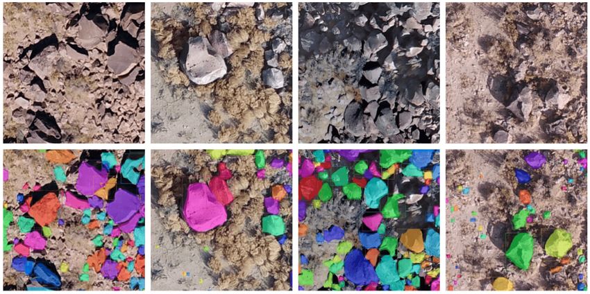
the first, proof-of-concept experiment with a DJI Phantom 4 Fig. 1: Visualization of instance segmentation. Colors indicate rock
Pro equipped with an RGB camera and inspected if elevation sizes. (A) Partial enlargement of the black rectangle in B. (B)
information assisted instance segmentation from RGB channels. Instance segmentation at the study area I. (C) Ground view after
Rock-trait histograms along and across the fault scarp were loading the GeoTiff image into Google Earth.
obtained with the neural network inference. In the second
experiment, we deployed a hexrotor and a multispectral camera cm-scale orthomosaics. Such data products require semi-
to produce a DEM and five spectral orthomosaics in red, green, automatic methods to yield interpretable information.
blue, red edge, and near infrared. We focused on examining
the effectiveness of different combinations of input channels in In recent years, deep neural networks have demonstrated
instance segmentation. unprecedented success in image classification, segmentation,
and object detection, leading to extensive application in
I. INTRODUCTION satellite and airborne image analysis. Compared with deep
learning applications with satellite imagery [5, 6], close-
Geographic Information Systems (GIS) have helped in- range UAS imagery with high resolution extends the use
tegrate a wide range of data sources, enabling efficient of deep learning to features of interest over a large range of
approaches for geological studies [1]. Traditionally, field feature sizes, ranging as low as a few centimeters. However,
surveys have been a gold standard for data collection due to directly using camera perspective images from UAS does not
low bias and high tolerance for ambiguity. However, there are provide precise georeference for features of interest, which
logistical constraints to field surveys, and findings may not be is essential in some applications, such as geological studies.
as unbiased as previously assumed [2]. Meanwhile, remote Our work is motivated by the need for precise, large
sensing for the collection of close-range terrestrial data has spatial-scale estimation of geomorphological features. In this
evolved from traditional methods such as airplanes, balloons, study, we collect and process data that potentially correlate
and kites equipped with cameras and LiDARs to the use of with surface processes of tectonic fault scarps in Volcanic
versatile robotic platforms such as Unpiloted Aerial Vehicles Tablelands near Bishop, California [7]. Rock traits such
(UAV) or Unpiloted Aerial Systems (UAS) [3, 4]. Combining as size, roundness, and orientation are of importance in
data collection with UAV/UAS and Structure from Motion many surface process studies, including earthquake geology
(UAS-SfM) offers a low-cost solution for rapid mapping research. Rock size distributions in the field site reflect
of geologic sites, and generates data products like digital both the initial cooling joint fracture geometry and the
surface models (DSM), digital elevation models (DEM), and faulting-induced fracturing, which both vary with position
as a function of strain magnitude and linkage characteristics.
Authors are affiliated with the School of Earth and Space Exploration,
Arizona State University, 781 Terrace Mall, Tempe, AZ 85287, USA In addition, impacts during transport and thermal cycling
{zch,ramon.arrowsmith,jnaneshwar.das}@asu.edu may further drive fracturing and influence the particle sizes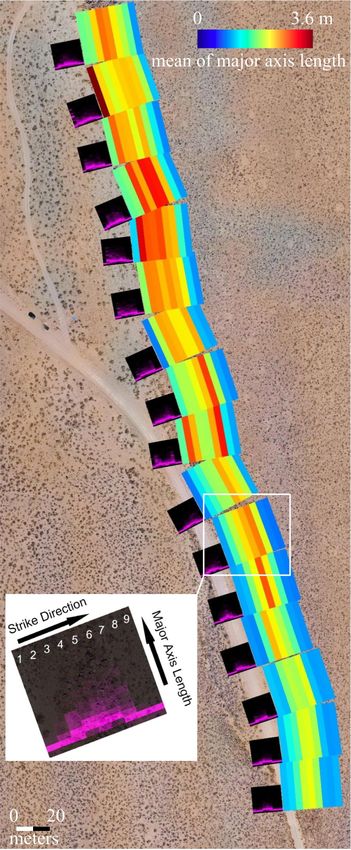
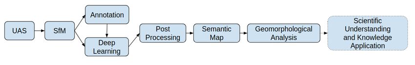
Fig. 2: Workflow of UAS-SfM-DL. The presented pipeline expands the utilities of models from UAS-SfM.

and shapes [8]. Rock orientations indicate the character
of downslope transport along the fault scarps, enhancing
our understanding of erosional processes. Current analyses
of topographic or imagery-based models produced by SfM
largely rely on experts manually annotating features of
interest (rocks).
   We present a pipeline that combines UAS, SfM, and deep
learning (UAS-SfM-DL) to produce high-resolution semantic
maps of objects, such as rocks, with wide variation in size
and appearance (Fig. 2). We show that deep learning can
be effectively applied to products from SfM, which may
contain artifacts resulting from reconstruction. Advantages
                                                                    Fig. 3: Areas of study and UAVs. (A) Areas of study. The top-right
of the presented system include low-cost, rapid deployment
                                                                    rectangle: experiment I; the bottom-left rectangle: experiment II.
and analysis, and automated processing with limited expert          (B) DJI Phantom 4 Pro with an RGB camera. (C) Hexrotor with a
intervention. In comparison with deep learning methods on           MicaSense RedEge MX.
perspective UAS imagery [9], the UAS-SfM-DL paradigm
can produce consistent georeferenced semantic maps (e.g.
                                                                    availability of low cost UAS and software such as Agisoft
Fig. 1), enabling large-scale, precise spatial analysis. The
                                                                    [11], UAS-SfM have widely been used in physical geography
map size, however, increases significantly when applying
                                                                    [12] ranging from coastal environments [13], to Antarctic
deep neural networks on large orthomosaics. Instead of
                                                                    moss beds [14], to fault scarps [15, 16]. However, geomor-
relying on expensive computation, we propose an affordable
                                                                    phological analysis of products from UAS-SfM still depends
solution that trains and infers on small tiles split from a large
                                                                    a lot on interpretive models carefully designed by experts
map. We present a registration algorithm to merge semantic
                                                                    [17, 18].
objects from multiple tiles during inference.
   We applied the UAS-SfM-DL system to two experiments              B. Deep Learning in Close-range Aerial Imagery Processing
analyzing rock traits along a tectonic fault scarp in Bishop,          The advances in deep learning have facilitated the devel-
California (Fig. 3). In the first experiment, we deployed a         opment of visual perception models deployed aboard UAS
DJI Phantom 4 Pro with an RGB camera to demonstrate                 as well as ground vehicles in various applications like weed
proof of concept, and inspected how much elevation infor-           classification [19], car detection [9], and fruit counting [20].
mation improved instance segmentation from RGB channels.            However, previous work largely targets camera perspective
In the second experiment, we equipped a hexrotor with a             imagery as the input to the deep learning models. Although
multispectral camera (MicaSense RedEdge MX) that can                feature tracking algorithms [21] can reconstruct objects of
capture spectral imagery from five bands: red (R), green            interest, they lack ground control points (GCPs) to globally
(G), blue (B), red edge (RE), and near infrared (NIR). The          correct geographic distortions, which is an essential step
orthomosaics of the five channels and the DEM acquired              in geological and surveying applications. Deep learning has
from SfM were used to train a deep neural network to                also been used to process 3D information, such as LiDAR
detect and segment individual rocks. We compared the neural         point clouds. For example, point cloud data generated from
network inference performance for different input channel           scanning trees were processed by fully connected layers for
combinations. This UAS-SfM-DL system presents a new                 tree classification [22].
way to automatically characterize surface processes on fault
scarps.                                                                              III. S YSTEM D ESCRIPTION
                                                                       The workflow of our UAS-SfM-DL pipeline is shown in
                     II. R ELATED W ORK
                                                                    Fig. 2. Although each component in the pipeline is not new,
A. Unpiloted Aircraft Systems and Structure from Motion             we focus on system integration and solutions to practical
(UAS-SfM)                                                           implementation issues involved in this fault scarp application
  Structure from motion originated in the computer vision           in geomorphological analysis. Additionally, we present the
community and has become popular with the utilization               pipeline from a high-level perspective to avoid curbing the
of bundle adjustment optimization [10]. With the recent             generalization to other potential applications.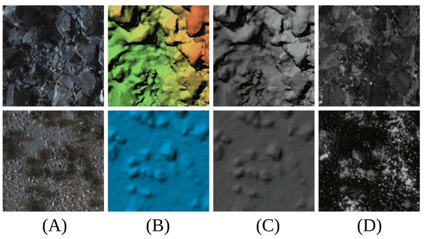
fault scarp. Additionally, because of the large range of rock
                                                                     sizes (major-axis lengths ranging between 0.2-3.6 meters),
                                                                     we select the Pyramid Feature Network (PFN) [26] as the
                                                                     backbone of the Faster R-CNN. PFN’s multi-scale, pyramidal
                                                                     hierarchy of anchor generation mechanism is suitable for
                                                                     object detection in such a setting. For other potential studies,
                                                                     segmentation neural networks such as U-Net [27] can be used
                                                                     when a goal is a pixel-level segmentation. Region proposal
                                                                     networks such as Faster R-CNN [25] can detect individual
                                                                     objects with bounding boxes, when instance segmentation is
Fig. 4: Spectral and DEM representations. All tiles on each row      not demanded.
are of the same area. Column (A) RGB orthomosaic tiles. Column          While it is common to scale spectral orthomosaics by
(B) Colormap elevation tiles. Column (C) Relative elevation tiles.   intensity values, directly scaling DEM by elevation range
Column (D) NDVI orthomosaic tiles.
                                                                     values will overshadow the rock information in the scaled
                                                                     space. This is because the fault scarp slope elevation (20-30
   Aerial imagery from UAS along with GCPs are processed             meters) is greater than the height of most of the rocks (0.2-
using SfM algorithms to reconstruct a high-resolution study          3 meters). Instead of compressing elevation into one single
site. Geologists annotate features of interest, such as rock         channel, we use a colormap (3 channels) to encode the DEM:
boundaries, from a portion of the RGB orthomosaics. We
train deep neural networks on annotated images, and carry                                    Drgb = c(s(h))                       (1)
out inference on unlabelled images from the entire site.             where h is absolute elevation, s is a linear scale function
Segmented objects inferred by the deep learning models are           s : [hmin , hmax ] → [0, 1], and c is a colormap function mapping
post-processed by geometric structural analysis and shape            scaled value to RGB color domain c : [0, 1] → {r, g, b}. In
descriptors to estimate properties such as rock size, round-         doing so, we capture the rock elevation in the three channels
ness, and orientation. We generate semantic maps by combin-          so that the rock height will not be overshadowed. An example
ing the post-processed inference results with georeferenced          of jet colormap is shown in Fig. 4(B). Because colormap
metadata. Statistics describing the distribution of rock traits      elevation represents absolute elevation, one concern is that
are acquired from the semantic maps, and they can be used in         deep learning networks may be constrained to learn features
statistical descriptions for future geomorphological studies.        only from a certain range of absolute elevation. This issue
A. UAS-SfM                                                           may become more serious in this study because the number
                                                                     of rocks on the fault scarp is greater than the number of
   Georeferenced aerial imagery collected from UAS and               rocks on the lower-side hanging wall.
GCPs measured from differential GPS devices are pro-                     Apart from colormap elevation, we present another eleva-
cessed by bundle-adjustment-based SfM algorithms [23],               tion representation that preserves local, relative elevation:
which produce precise georeferenced products including
point clouds, DEM, DSM, and orthomosaics for each spectral                                            Dr Dg Db
                                                                                     D = g(Drgb ) =      +      +                 (2)
band. In practice, the orthomosaics and DEM are formatted                                              3     3     3
as GeoTiff files with metadata such as global coordinates,           where Dr , Dg , and Db are three channels from Drgb . The
projection type, and ground resolution. These data give us           relative elevation representation (Fig. 4(C)) is superior in the
access to global coordinates of each 3D point or pixel in            sense that it can reflect local elevation such that deep neural
the models, which enables succeeding spatial analysis of             networks can attain generalization to detect and segment
semantic features from deep learning.                                rocks on any elevations. One potential concern of relative
                                                                     elevation is that the mapping g(c(s(·))) is noncontinuous
B. Deep Learning                                                     on the absolute elevation domain, which may result in
   We use deep neural networks to automatically extract              high-frequency noises in relative elevation tiles. However,
semantic information in large-scale georeferenced models             our experiments in the next section show that such high-
produced from SfM. Deep learning accommodates versatile,             frequency noises will not cause problems for deep neural
selectable inputs such as RGB orthomosaics, DEMs, and                networks.
other spectral orthomosaics from multispectral cameras. The
selection of neural network architecture depends on the              C. Tiling and Registration
features and distributions of objects of interest. We use the           The orthomosaics of survey sites produced by SfM are
Mask R-CNN deep neural network architecture [24] for this            of high resolution and large scale (for our first fault scarp
study because it generates both bounding boxes and the               study, 2 cm/pixel, 25664x10589 pixels). Directly working
corresponding masks for object instances (rocks). Faster R-          with high-resolution images for neural network training or
CNN [25] with a large number of Regions of Interest is               inference is computationally challenging because it places a
adopted for the object detection branch in the Mask R-CNN            high demand on GPU RAM. To address this limitation, we
because of the dense spatial distribution of the rocks at this       split the orthomosaics into smaller tiles (400x400 pixels).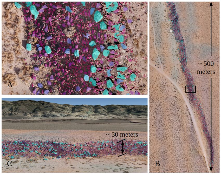
Fig. 5: Rock registration at tile boundaries. (Left) Rocks detected by
the neural network at the edges of each inference are not merged;
(right) any two rocks at the edges of each inference are merged and
registered as one if they belong to the same instance.
 Algorithm 1 Rock Registration
 input: orthomosaics, neural_network
 output: registered_rocks                                                      Fig. 6: Identifying the fault scarp. (A) Slope map. (B) Fault scarp
 1. tiles = overlap_split(orthomosaics)                                        contour. (C) Overlap with RGB orthomosaics.
 2. rocks = project(neural_network(tiles))
 3. registered_rock = Empty_list
 4. for rock in rocks:
        if rock.bbox is on its own tile edges:
             id = check_bbox_overlap(rock.bbox, registered_rocks)
             if id 6= None:
                 if check_mask_overlap(rock.mask, registered_rocks[id].mask)
                     > threshold:
                      merge(registered_rocks[id], rock)
                      continue                                                 Fig. 7: Contour analysis to compensate for instability of segmen-
         register(registered_rocks, rock)                                      tation prediction. (A) Mask prediction from Mask R-CNN. (B)
 Comments:                                                                     Contours by topological structure analysis. (C) The largest contour
 overlap_split splits orthomosaics into 400x400 pixel tiles with 10-pixel      kept to approximate outline of the rock. (D) Filtered mask.
 overlap at four edges
 project projects local bounding boxes with pixel coordinates to global
 coordinates
 check_bbox_overlap returns None if there is no registered rocks having
                                                                               D. Post Processing
 bounding box overlap with the rock, otherwise returns the overlapped             Post processing is necessary to identify the rocks on the
 registered rock’s id
 check_mask_overlap returns the intersection of two masks                      fault scarp, and to compensate for errors resulting from deep
 merge merges the bounding boxes and masks to the registered rock              neural networks. Because only rocks near the fault scarp are
 register registers a new rock
                                                                               of interest for tectonic study, we need to clear away rocks
                                                                               detected on the perimeter. As the fault scarp has a steep slope,
                                                                               we first estimate the gradient of the DEM [29], then denoise
We select a subset of tiles and annotate rocks as bounding                     it with Gaussian filtering. From the smoothed slope map, the
polygons in LabelMe [28], then divide them into a training                     fault scarp is identified by the slope above a certain threshold
dataset and a testing dataset. We augment the training dataset                 and further processed through morphological transformations
with a combination of random left-right flipping, top-down                     such as opening, dilation, erosion, etc.
flipping, rotation, and zooming-in (cropping) and zooming-                        The segmentation sub-network has stochastic errors, with
out.                                                                           an example shown in Fig. 7(A) where a hole is present
   Splitting the orthomosaics into tiles causes some rocks to                  in the segmented rock body. We assume that there are
be divided. As a result, rocks detected at the edges of tiles                  no rocks with torus topology on the fault scarp, and use
may belong to one single instance and risk getting treated as                  topological structure analysis to remove such artifacts [30].
several smaller rocks as shown in Fig. 5(right). To address                    The contours of rocks are generated, with the largest or most
this problem, we split the orthomosaics into 400x400 pixel                     exterior contours retained as the outlines of the rocks. The
tiles with 10-pixel overlaps on four edges when carrying                       rock sizes are approximated by the number of pixels in the
out inference. A registration scheme is applied to merge                       largest contours. Note that georeferenced models enable us to
objects detected at the edges of tiles if they are from a single               associate rock size in pixels and rock size in meters, which
instance (Algorithm I). We determine that two georeferenced                    is more accurate than the association from perspective 2D
rock instances within the 10-pixel region of overlap are the                   camera photos where object scale is ambiguous with depth.
same instance by checking if the intersection of their masks
is greater than a threshold. If true, the two rock instances                                         IV. E XPERIMENTS
are merged and registered as one instance (Fig. 5(left)). To                     In this section, we discuss the results of our pipeline
keep the comparison in check_bbox_overlap from becoming                        in two experiments at the Volcanic Tablelands, which is
quadratic with rock numbers, we utilize the spatial relation                   a faulted plateau of approximately 150-meter-thick welded
and only compare rock overlaps for rocks on the 10-pixel                       Bishop Tuff (760 ka) at the north end of Owens Valley near
overlap zones of four neighbor tiles.                                          Bishop, California [7].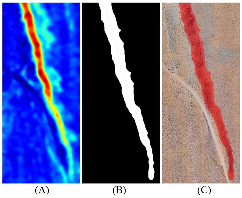
TABLE I: Experiment I: Neural Network Inference Results*
                                                        Detection                                      Segmentation
                                                     (Bounding Box)                                       (Mask)
                                       AP1     AP2     AP3     AP4     AR1     AR2     AP1      AP2     AP3     AP4    AR1    AR2
                  1 RGB                21.7    46.5    17.0    36.9    31.4    48.3    20.8     46.5 14.6       48.6   29.8   51.7
          TL      2 RGB+DEM3 22.7              45.3    19.4    51.1    32.1    58.3    21.2     45.7 16.4       50.7   30.3   53.3
                  3 RGB+DEM1 23.1              46.9    20.5    53.9    32.6    58.3    25.1     47.4 16.2       61.0   30.8   65.0
                  4 RGB                21.2    46.2    16.5    42.9    29.9    43.3    21.2     45.7 16.3       42.9   29.3   50.0
         NTL 5 RGB+DEM3 20.5                   42.6    16.6    40.2    29.9    45.0    19.4     42.4 14.6       48.6   28.1   53.3
                  6 RGB+DEM1 21.4              45.9    16.1    40.6    30.9    48.3    21.6     46.6 16.5       49.9   31.0   56.7
         * TL: transfer learning, NTL: no transfer learning, IoU: intersection over union, AP1 : average precision (%) with
         IoU=0.5:0.95, AP2 : average precision (%) with IoU=0.5, AP3 : average precision (%) with IoU=0.75, AP4 : average
         precision (%) with IoU=0.5:0.95 for large objects, AR1 : average recall (%) with IoU=0.50:0.95,
         AR2 : average recall (%) with IoU=0.50:0.95 for large objects

                                                                       Fig. 9: Ellipse fitting and estimation of major orientations from the
                                                                       inferred rock boundaries. Yellow line indicates major axis.

                                                                       and segmentation), RGB+DEM1 outperformed others in both
                                                                       transfer learning and non-transfer learning.
Fig. 8: Prediction of Mask R-CNN on test dataset sample tiles.
Colors are randomly selected to distinguish rocks.                         Once neural network inference was conducted on all tiles
                                                                       from the study area, we carried out post-processing to obtain
                                                                       rock-trait histograms at the fault scarp. We removed outliers
A. DJI Phantom 4 Pro and RGB Camera                                    on the perimeter and identified the boundaries of the fault
   The study area for the first experiment is shown in the top-        scarp from the slope map utilizing terrain gradient. The slope
right rectangle in Fig. 3(A). One goal of this experiment is           map and the fault scarp contour are shown in Fig. 6. The
to demonstrate the proof of concept by going through imple-            enclosed rocks were then estimated by the refined masks
mentation details in the presented pipeline and obtaining the          from topological structure analysis. The results of the filtered
rock-trait histograms. We conducted surveys of the Volcanic            rock instances at the fault scarp of this study area are shown
Tablelands with a DJI Phantom 4 Pro in March 2018. A grid              in Fig. 1. Some predictions randomly selected from the test
flight pattern was implemented with 66% image overlap and              dataset are shown in Fig. 8.
a 90° (nadir) camera angle. The flight altitude varied between             Lastly, we used the georeferenced rock boundary informa-
70-100 meters above the ground level because the height of             tion to estimate rock diameter, roundness, and orientation. To
the fault scarp slope is around 30 meters. The onboard RGB             approximate roundness and major orientations of rocks, we
camera had an 84° field of view and 5472x3648 resolution.              fitted the refined masks with ellipses as shown in Fig. 9.
   We used Agisoft [11] for SfM and produced a DEM and                 We used ellipse eccentricity to describe rock roundness. The
an RGB orthomosaic (25664x10589 pixels, 2 cm/pixel). The               orientations of rocks were parameterized by orientations of
orthomosaics were split into 400x400 tiles. It took about 65           the ellipses’ major axes. Fig. 10 shows rock-trait histograms
work hours for a human expert to annotate 67 tiles with                of the fault scarp. In this experiment, 12,682 rocks were
4095 rocks (49 tiles for training, and 18 for testing). We             detected along the fault scarp in the study area, which only
trained Mask R-CNN (ResNet-50 backbone) on an Nvidia                   has an area of 513 meters by 212 meters.
RTX 2080 Ti, and the inference results on the test dataset                 We are not only interested in the distribution of rock traits
are shown in Table I.                                                  along the length of the scarp, but along the cross strike
   For transfer learning, the neural network weights were              as well, which is the perpendicular direction of the fault
initialized with training results from COCO 2017, except               scarp (Fig. 11). We computed the skeleton of the fault scarp
that the first and the last layers were initialized from a             contour to acquire the middle spline [31], then selected a
uniform distribution. When comparing trials between TL                 subsection of the spline and approximated it with a straight
and NTL (Table I), we found the neural networks benefited              line by linear regression. We considered the normal vector of
from transfer learning. Both colormap elevation (DEM3)                 the straight line as the cross strike direction. The whole fault
and relative elevation (DEM1) improved neural network                  scarp is divided into 16 areas that are lying in the center
performance from RGB orthomosaics in the case of transfer              of the spline. Each area is divided into 9 boxes along the
learning. DEM3 assisted the neural network performance                 cross strike direction. Within each box, there are 20 bins
in transfer learning but decreased in non-transfer learning.           representing the normalized rock diameter histogram in the
Considering key performances (AP1 , AR1 for both detection             true box. From the bottom (south) to top (north) in each area,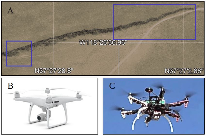
Fig. 10: Histograms of rock traits. (A) Rock size histogram of the
fault scarp. The rock sizes are approximated by the area of the
refined masks. The horizontal axis is rock area in meters2 , and the
vertical axis is the number of rocks. (B) Rock eccentricity histogram
of the fault scarp. (C) Rock major-axis length histogram on the fault
scarp. The major-axis length is L = 2a, where a is the semimajor
                              2     2
axis of the fitting ellipse ax2 + by2 = 1. (D) Polar histogram of major-
axis orientation at the fault scarp.

the histogram axis (major-axis length) varies from 0 to 3.6
meters.

B. Hexrotor and Multispectral Camera
   In this experiment, we focused on examining the presented
pipeline on different combinations of inputs including multi-
spectral orthomosaics, color elevation, and relative elevation.
The study area for this experiment is shown in the bottom-left
rectangle in Fig. 3(A). We equipped a hexrotor with an RTK
GPS and a straight-down multispectral camera (MicaSense
RedEdge MX) that can capture spectral bands of blue (465-
485 nm), green (550-570 nm), red (663-673 nm), red edge
(712-722 nm), and near infrared (820-860 nm). We deployed
a lawnmower pattern with a flight altitude of 30-50 meters
above the fault scarp (the height of the fault scarp slope is
about 20 meters) and collected synchronized multispectral
imagery in April 2019. Agisoft [11] was used for SfM and
produced a DEM and five spectral orthomosaics (9258x8694
pixels, 2 cm/pixel). We split the spectral orthomosaics and
DEM into 400x400 tiles with 10-pixel size overlap at four
edges. It took about 50 work hours for a human expert to                   Fig. 11: Detailed rock diameter (major-axis length) histogram
annotate 37 tiles for training and 18 tiles for testing (2541              colormap for the study area. The colormap on the fault scarp shows
rocks annotated in total). We trained Mask R-CNN (ResNet-                  the mean rock diameter for each box along the scarp. The smaller
50 backbone) on an Nvidia RTX 2080 Ti.                                     black plots at the left show detailed histograms of rock diameter
   The inference results on the test dataset are shown in                  with transparency indicating lower spatial density.
Table II. We consider RGB results (trials 1 and 8) as
the baseline and discuss the neural network performances                   bushes in the site, e.g. Fig. 4. Relative elevation (DEM1)
with different input combinations. Because there are several               outperformed colormap elevation (DEM3) in trial 3 versus
different performance metrics in the table and neural network              trial 4, trial 10 versus trial 11, and trial 13 versus trial 14.
prediction can be noisy, we emphasize four key metrics - AP1               Though from trial 6 versus trial 7 these two elevation repre-
and AR1 from detection and segmentation.                                   sentations had comparable improvements, relative elevation
   1) DEM: Additional elevation information improved the                   showed slight advances in key metrics.
performance by the comparisons of trial 3/4 versus trial 1,                   2) Multispectral orthomosaics: RE and NIR can reveal
and trial 10/11 versus trial 8. Elevation information alone,               information that RGB alone cannot obtain. For example,
however, only worked for the detection and segmentation of                 normalized difference vegetation index (NDVI) has largely
large rocks, which may be caused by the comparable-size                    been used for vegetation detection. An example of NDVI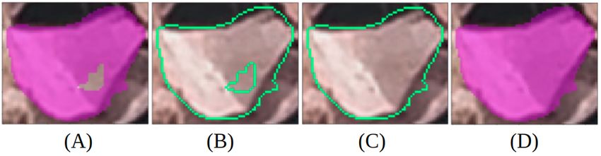
TABLE II: Experiment II: Neural Network Inference Result*
                                                                 Detection                                 Segmentation
                                                              (Bounding Box)                                  (Mask)
                                                AP1    AP2      AP3     AP4    AR1    AR2    AP1    AP2     AP3   AP4     AR1    AR2
                  1    RGB                      25.7   60.7     17.2   51.9    37.0   57.0   23.4   51.8   15.3 52.9      27.8   55.0
                  2    DEM1                     4.9    15.3     2.3    39.5    11.2   58.0   4.3    12.5   2.0    45.5    9.9    53.0
                  3    RGB+DEM3                 28.4   64.0     19.7   64.9    39.5   69.0   26.6   61.6   18.7 61.1      36.3   62.0
          TL      4    RGB+DEM1                 28.8   64.7     22.1   59.1    40.1   63.0   26.8   61.8   19.1 54.5      36.3   56.0
                  5    RGB+RE+NIR               28.5   61.7     22.2   58.8    38.8   61.0   25.8   57.2   20.1 57.1      35.1   58.0
                  6    RGB+RE+NIR+DEM3          29.6   63.4     23.7   60.2    39.1   64.0   29.0   62.0   22.1 54.9      37.7   56.0
                  7    RGB+RE+NIR+DEM1          29.7   64.7     23.7   58.3    40.6   63.0   28.3   61.6   21.0 54.4      38.2   56.0
                  8    RGB                      24.9   60.4     16.1   40.2    34.2   45.0   22.5   55.9   14.3 43.5      31.2   45.0
                  9    DEM1                     3.8    11.5     1.8    31.7    8.7    45.0   3.3    9.8    1.1    31.1    7.3    36.0
                 10 RGB+DEM3                    26.0   62.3     17.9   45.0    36.0   55.0   24.1   57.4   16.3 51.6      33.6   54.0
         NTL 11 RGB+DEM1                        27.1   63.8     19.0   36.6    38.5   41.0   25.2   62.0   16.2 44.4      35.5   45.0
                 12 RGB+RE+NIR                  27.6   63.5     18.7   41.5    39.3   47.0   23.5   59.6   14.6 49.1      34.2   51.0
                 13 RGB+RE+NIR+DEM3             26.9   63.5     17.0   32.1    38.8   37.0   23.2   59.3   14.3 30.6      34.0   30.0
                 14 RGB+RE+NIR+DEM1             28.0   65.8     17.8   40.0    39.3   41.0   25.8   62.2   16.7 47.7      35.7   49.0
         * Refer to the table note in Table I

tiles is shown in Fig. 4(D). While NDVI was not directly                 the larger particles are typically in the mid scarp position.
used in our experiment, we included original RE and NIR                  Such information can guide future scientific inquiries about
in the input and let the neural networks mine the multi-                 strain across the fault as well as geomorphic modifications of
spectral orthomosaics themselves. RE+NIR assisted neural                 fault scarps to better understand earthquake recurrence in a
network performance when added to RGB, RGB+DEM3,                         tectonically active region. As far as we know, this is the first
and RGB+DEM1 in both transfer learning and non-transfer                  time that UAVs and machine learning are used to measure
learning.                                                                rock traits on fault scarps.
   3) Transfer learning: The trials with transfer learning                  In the second experiment, we focused on examining the
generally outperformed the ones without transfer learning                effectiveness of different input combinations of multispectral
with the exception of some acceptable noises in AP2 . Consid-            orthomosaics and two elevation representations. From the
ering key metrics, transfer learning did demonstrate advances            inference results, additional spectral data and elevation in-
in the inference performances.                                           formation improved the performance of the neural networks.
   4) DEM       and      Multispectral     orthomosaics:                 Even though the first convolutional layer of Mask R-CNN
RGB+RE+NIR+DEM3/RGB+RE+NIR+DEM1                        yielded           needed to be retrained, transfer learning showed general ad-
better results than other trials. While in transfer learning             vances over non-transfer learning in all combination settings.
RGB+RE+NIR+DEM1 was slightly better at key metrics, it                      Field inspection of the fault scarp indicated that the grain
surpassed other trials in non-transfer learning.                         size of the rocks included those smaller than the mode of
                                                                         0.2 meters (Fig. 10(C)). The rollover in grain size to the
         V. C ONTRIBUTION AND F UTURE W ORK                              smaller side is therefore likely due to a sensitivity issue from
                                                                         both image resolution (2-cm pixels for orthomosaics) and
   In this paper, we presented a pipeline for geomorpholog-
                                                                         neural network architectures. Addressing the finer size tail
ical analysis using structure from motion and deep learning
                                                                         on the rock size distribution is an important topic for future
on close-range aerial imagery. Our UAS-SfM-DL pipeline
                                                                         research.
was used to assess the effectiveness of multispectral data
                                                                            Rock sizes are approximated using 2D areas from ortho-
and elevation representations in neural networks and to
                                                                         mosaics. We will look at rock size estimation from 2.5D
estimate the distribution of rock traits (size, roundness, and
                                                                         (elevation) and 3D (point cloud) approaches. In this work,
orientation) on a fault scarp in the Volcanic Tablelands,
                                                                         we simply stack all different data as input and implicitly
California. Although presented in the context of fault zone
                                                                         rely on neural networks to learn useful features from in-
geology, we foresee our pipeline being extended to a variety
                                                                         put channels for instance segmentation. We will investigate
of geomorphological analysis tasks in other domains such as
                                                                         attention mechanism to actively weight interesting input
crop property estimation in precision agriculture and debris
                                                                         channels, which will benefit deep neural network learning
field analysis after natural disasters.
                                                                         in multispectral and hyperspectral data.
   From our first, proof-of-concept experiment, we conclude
that relative elevation improved the neural network per-                                     ACKNOWLEDGEMENTS
formance in both transfer learning and non-transfer learn-                 This work was supported in part by Southern California
ing. With transfer learning, we have shown both elevation                Earthquake Center (SCEC) award 19179, National Science
representations assisted neural network performance from                 Foundation award CNS-1521617, and National Aeronautics
RGB data, and the relative elevation resulted in the best                and Space Administration STTR award 19-1-T4.01-2855.
improvement. We also obtained rock-trait histograms along                Thank you to Duane DeVecchio for discussion on the ge-
and across the fault scarp. The distributions of rock size               omorphic concepts presented here.
are asymmetrical throughout the fault, with larger rocks
in the north and smaller rocks in the south. Additionally,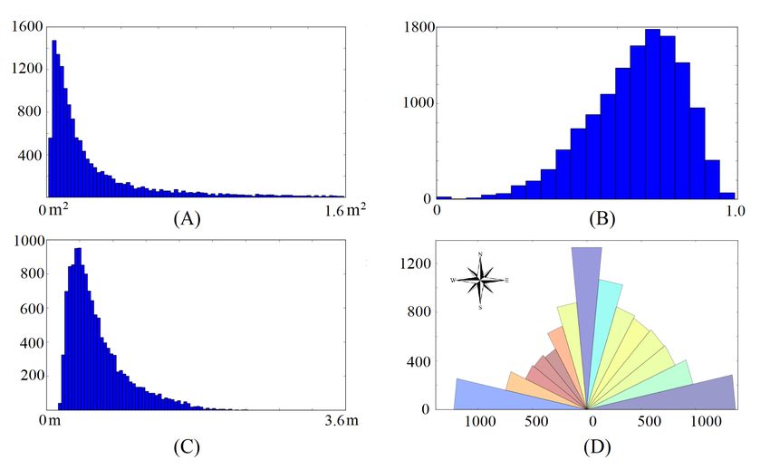
R EFERENCES                                  [17]   K. L. Cook. “An evaluation of the effectiveness of low-cost
 [1]   M. F. Goodchild. “Twenty years of progress: GIScience in               UAVs and structure from motion for geomorphic change
       2010”. In: Journal of spatial information science 2010.1               detection”. In: Geomorphology 278 (2017), pp. 195–208.
       (2010), pp. 3–20.                                               [18]   M. Bunds, C. Scott, N. Toke, R. Arrowsmith, J. Saldivar,
 [2]   J. B. Salisbury, D. Haddad, T. Rockwell, J. R. Arrowsmith,             L. Woolstenhulme, J. Phillips, S. Janecke, and J. Evans.
       C. Madugo, O. Zielke, and K. Scharer. “Validation of                   “Three dimensional aseismic creep deformation from differ-
       meter-scale surface faulting offset measurements from high-            encing of Structure from Motion and LiDAR high resolution
       resolution topographic data”. In: Geosphere 11.6 (2015),               topography on the San Andreas Fault, California”. In: AGU
       pp. 1884–1901.                                                         Fall Meeting Abstracts. 2018.
 [3]   J. Das, W. C. Evans, M. Minnig, A. Bahr, G. S. Sukhatme,        [19]   C. Hung, Z. Xu, and S. Sukkarieh. “Feature learning based
       and A. Martinoli. “Environmental sensing using land-based              approach for weed classification using high resolution aerial
       spectrally-selective cameras and a quadcopter”. In: Experi-            images from a digital camera mounted on a UAV”. In:
       mental Robotics. Springer. 2013, pp. 259–272.                          Remote Sensing 6.12 (2014), pp. 12037–12054.
 [4]   J. Das, G. Cross, C. Qu, A. Makineni, P. Tokekar, Y.            [20]   S. W. Chen, S. S. Shivakumar, S. Dcunha, J. Das, E. Okon,
       Mulgaonkar, and V. Kumar. “Devices, systems, and methods               C. Qu, C. J. Taylor, and V. Kumar. “Counting apples and
       for automated monitoring enabling precision agriculture”. In:          oranges with deep learning: A data-driven approach”. In:
       2015 IEEE International Conference on Automation Science               IEEE Robotics and Automation Letters 2.2 (2017), pp. 781–
       and Engineering (CASE). IEEE. 2015, pp. 462–469.                       788.
 [5]   X. X. Zhu, D. Tuia, L. Mou, G.-S. Xia, L. Zhang, F. Xu, and     [21]   X. Liu, S. W. Chen, C. Liu, S. Skandan, J. Das, C. J. Taylor,
       F. Fraundorfer. “Deep learning in remote sensing: A compre-            J. P. Underwood, and V. Kumar. “Monocular camera based
       hensive review and list of resources”. In: IEEE Geoscience             fruit counting and mapping with semantic data association”.
       and Remote Sensing Magazine 5.4 (2017), pp. 8–36.                      In: IEEE Robotics and Automation Letters (2019).
 [6]   N. Kussul, M. Lavreniuk, S. Skakun, and A. Shelestov.           [22]   H. Guan, Y. Yu, Z. Ji, J. Li, and Q. Zhang. “Deep learning-
       “Deep learning classification of land cover and crop types             based tree classification using mobile LiDAR data”. In:
       using remote sensing data”. In: IEEE Geoscience and Re-                Remote Sensing Letters 6.11 (2015), pp. 864–873.
       mote Sensing Letters 14.5 (2017), pp. 778–782.                  [23]   B. Triggs, P. F. McLauchlan, R. I. Hartley, and A. W.
 [7]   D. A. Ferrill, A. P. Morris, R. N. McGinnis, K. J. Smart,              Fitzgibbon. “Bundle adjustment—a modern synthesis”. In:
       M. J. Watson-Morris, and S. S. Wigginton. “Observations                International workshop on vision algorithms. Springer. 1999,
       on normal-fault scarp morphology and fault system evolution            pp. 298–372.
       of the Bishop Tuff in the Volcanic Tableland, Owens Valley,     [24]   K. He, G. Gkioxari, P. Dollár, and R. Girshick. “Mask R-
       California, USA”. In: Lithosphere 8.3 (2016), pp. 238–253.             CNN”. In: Proceedings of the IEEE international conference
 [8]   L. McFadden, M. Eppes, A. Gillespie, and B. Hallet. “Phys-             on computer vision. 2017, pp. 2961–2969.
       ical weathering in arid landscapes due to diurnal variation     [25]   S. Ren, K. He, R. Girshick, and J. Sun. “Faster R-CNN:
       in the direction of solar heating”. In: Geological Society of          Towards real-time object detection with region proposal
       America Bulletin 117.1-2 (2005), pp. 161–173.                          networks”. In: Advances in neural information processing
 [9]   N. Ammour, H. Alhichri, Y. Bazi, B. Benjdira, N. Alajlan,              systems. 2015, pp. 91–99.
       and M. Zuair. “Deep learning approach for car detection in      [26]   T.-Y. Lin, P. Dollár, R. Girshick, K. He, B. Hariharan, and S.
       UAV imagery”. In: Remote Sensing 9.4 (2017), p. 312.                   Belongie. “Feature pyramid networks for object detection”.
[10]   N. Snavely, I. Simon, M. Goesele, R. Szeliski, and S. M.               In: Proceedings of the IEEE Conference on Computer Vision
       Seitz. “Scene reconstruction and visualization from commu-             and Pattern Recognition. 2017, pp. 2117–2125.
       nity photo collections”. In: Proceedings of the IEEE 98.8       [27]   O. Ronneberger, P. Fischer, and T. Brox. “U-net: Convo-
       (2010), pp. 1370–1390.                                                 lutional networks for biomedical image segmentation”. In:
[11]   Agisoft. https://www.agisoft.com/. 2018.                               International Conference on Medical image computing and
[12]   M. J. Westoby, J. Brasington, N. F. Glasser, M. J. Hambrey,            computer-assisted intervention. Springer. 2015, pp. 234–241.
       and J. Reynolds. “‘Structure-from-Motion’photogrammetry:        [28]   B. C. Russell, A. Torralba, K. P. Murphy, and W. T. Freeman.
       A low-cost, effective tool for geoscience applications”. In:           “LabelMe: A database and web-based tool for image anno-
       Geomorphology 179 (2012), pp. 300–314.                                 tation”. In: International journal of computer vision 77.1-3
[13]   F. Mancini, M. Dubbini, M. Gattelli, F. Stecchi, S. Fabbri,            (2008), pp. 157–173.
       and G. Gabbianelli. “Using unmanned aerial vehicles (UAV)       [29]   B. K. Horn. “Hill shading and the reflectance map”. In:
       for high-resolution reconstruction of topography: The struc-           Proceedings of the IEEE 69.1 (1981), pp. 14–47.
       ture from motion approach on coastal environments”. In:         [30]   S. Suzuki et al. “Topological structural analysis of digitized
       Remote Sensing 5.12 (2013), pp. 6880–6898.                             binary images by border following”. In: Computer vision,
[14]   A. Lucieer, S. A. Robinson, and D. Turner. “Unmanned                   graphics, and image processing 30.1 (1985), pp. 32–46.
       aerial vehicle (UAV) remote sensing for hyperspatial terrain    [31]   T. Zhang and C. Y. Suen. “A fast parallel algorithm for
       mapping of Antarctic moss beds based on structure from                 thinning digital patterns”. In: Communications of the ACM
       motion (SfM) point clouds”. In: (2011).                                27.3 (1984), pp. 236–239.
[15]   A. Donnellan, J. Green, A. Ansar, R. Muellerschoen, J.
       Parker, A. Tanner, Y. Lou, M. Heflin, R. Arrowsmith, J.
       Rundle, et al. “Geodetic imaging of fault systems from
       airborne platforms: UAVSAR and Structure from Motion”.
       In: IGARSS 2018-2018 IEEE International Geoscience and
       Remote Sensing Symposium. IEEE. 2018, pp. 7878–7881.
[16]   K. Johnson, E. Nissen, S. Saripalli, J. R. Arrowsmith, P.
       McGarey, K. Scharer, P. Williams, and K. Blisniuk. “Rapid
       mapping of ultrafine fault zone topography with structure
       from motion”. In: Geosphere 10.5 (2014), pp. 969–986.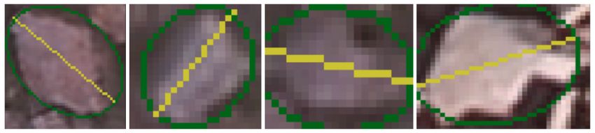
You can also read


