DC3: A LEARNING METHOD FOR OPTIMIZATION WITH HARD CONSTRAINTS
←
→
Page content transcription
If your browser does not render page correctly, please read the page content below
Published as a conference paper at ICLR 2021

                                         DC3: A LEARNING METHOD FOR OPTIMIZATION
                                         WITH HARD CONSTRAINTS

                                             Priya L. Donti1, * , David Rolnick2, * , J. Zico Kolter1,3
                                          1
                                             Carnegie Mellon University, 2 McGill University and Mila, 3 Bosch Center for AI
                                          pdonti@cs.cmu.edu, drolnick@cs.mcgill.ca, zkolter@cs.cmu.edu

                                                                                         A BSTRACT
arXiv:2104.12225v1 [cs.LG] 25 Apr 2021

                                                       Large optimization problems with hard constraints arise in many settings, yet clas-
                                                       sical solvers are often prohibitively slow, motivating the use of deep networks as
                                                       cheap “approximate solvers.” Unfortunately, naive deep learning approaches typ-
                                                       ically cannot enforce the hard constraints of such problems, leading to infeasible
                                                       solutions. In this work, we present Deep Constraint Completion and Correction
                                                       (DC3), an algorithm to address this challenge. Specifically, this method enforces
                                                       feasibility via a differentiable procedure, which implicitly completes partial so-
                                                       lutions to satisfy equality constraints and unrolls gradient-based corrections to
                                                       satisfy inequality constraints. We demonstrate the effectiveness of DC3 in both
                                                       synthetic optimization tasks and the real-world setting of AC optimal power flow,
                                                       where hard constraints encode the physics of the electrical grid. In both cases,
                                                       DC3 achieves near-optimal objective values while preserving feasibility.

                                         1        I NTRODUCTION
                                         Traditional approaches to constrained optimization are often expensive to run for large problems,
                                         necessitating the use of function approximators. Neural networks are highly expressive and fast
                                         to run, making them ideal as function approximators. However, while deep learning has proven
                                         its power for unconstrained problem settings, it has struggled to perform well in domains where it
                                         is necessary to satisfy hard constraints at test time. For example, in power systems, weather and
                                         climate models, materials science, and many other areas, data follows well-known physical laws,
                                         and violation of these laws can lead to answers that are unhelpful or even nonsensical. There is thus
                                         a need for fast neural network approximators that can operate in settings where traditional optimizers
                                         are slow (such as non-convex optimization), yet where strict feasibility criteria must be satisfied.
                                         In this work, we introduce Deep Constraint Completion and Correction (DC3), a framework for
                                         applying deep learning to optimization problems with hard constraints. Our approach embeds dif-
                                         ferentiable operations into the training of the neural network to ensure feasibility. Specifically, the
                                         network outputs a partial set of variables with codimension equal to the number of equality con-
                                         straints, and “completes” this partial set into a full solution. This completion process guarantees
                                         feasibility with respect to the equality constraints and is differentiable (either explicitly, or via the
                                         implicit function theorem). We then fix any violations of the inequality constraints via a differ-
                                         entiable correction procedure based on gradient descent. Together, this process of completion and
                                         correction enables feasibility with respect to all constraints. Further, this process is fully differen-
                                         tiable and can be incorporated into standard deep learning methods.
                                         Our key contributions are:
                                                     • Framework for incorporating hard constraints. We describe a general framework, DC3,
                                                       for incorporating (potentially non-convex) equality and inequality constraints into deep-
                                                       learning-based optimization algorithms.
                                                     • Practical demonstration of feasibility. We implement the DC3 algorithm in both convex
                                                       and non-convex optimization settings. We demonstrate the success of the algorithm in pro-
                                                       ducing approximate solutions with significantly better feasibility than other deep learning
                                                       approaches, while maintaining near-optimality of the solution.
                                              ∗
                                                  These authors contributed equally.

                                                                                               1
Published as a conference paper at ICLR 2021
• AC optimal power flow. We show how the general DC3 framework can be used to opti-
mize power flows on the electrical grid. This difficult non-convex optimization task must be
solved at scale and is especially critical for renewable energy adoption. Our results greatly
improve upon the performance of general-purpose deep learning methods on this task.
2 R ELATED W ORK
Our approach is situated within the broader literature on fast optimization methods, and draws inspi-
ration from literature on implicit layers and on incorporating constraints into neural networks. We
briefly describe each of these areas and their relationship to the present work.
Fast optimization methods. Many classical optimization methods have been proposed to improve
the practical efficiency of solving optimization problems. These include general techniques such as
constraint and variable elimination (i.e., the removal of non-active constraints or redundant variables,
respectively), as well as problem-specific techniques (e.g., KKT factorization techniques in the case
of convex quadratic programs) (Nocedal & Wright, 2006). Our present work builds upon aspects
of this literature, applying concepts from variable elimination to reduce the number of degrees of
freedom associated with the optimization problems we wish to solve.
In addition to the classical optimization literature, there has been a large body of literature in deep
learning that has sought to approximate or speed up optimization models. As described in reviews
on topics such as combinatorial optimization (Bengio et al., 2020) and optimal power flow (Hasan
et al., 2020), ML methods to speed up optimization models have thus far taken two main approaches.
The first class of approaches, akin to work on surrogate modeling (Koziel & Leifsson, 2013), has
involved training machine learning models to map directly from optimization inputs to full solu-
tions. However, such approaches have often struggled to produce solutions that are both feasible
and (near-)optimal. The second class of approaches has instead focused on employing machine
learning approaches alongside or in the loop of optimization models, e.g., to learn warm-start points
(see, e.g., Baker (2019) and Dong et al. (2020)) or to enable constraint elimination techniques by
predicting active constraints (see, e.g., Misra et al. (2018)). We view our work as part of the for-
mer set of approaches, but drawing important inspiration from the latter: that employing structural
knowledge about the optimization model is paramount to achieving both feasibility and optimality.
Constraints in neural networks. While deep learning is often thought of as wholly unconstrained,
in reality, it is quite common to incorporate (simple) constraints within deep learning procedures. For
instance, softmax layers encode simplex constraints, sigmoids instantiate upper and lower bounds,
ReLUs encode projections onto the positive orthant, and convolutional layers enforce translational
equivariance (an idea taken further in general group-equivariant networks (Cohen & Welling, 2016)).
Recent work has also focused on embedding specialized kinds of constraints into neural networks,
such as conservation of energy (see, e.g., Greydanus et al. (2019) and Beucler et al. (2019)), and
homogeneous linear inequality constraints (Frerix et al., 2020). However, while these represent
common “special cases,” there has to date been little work on building more general hard constraints
into deep learning models.
Implicit layers. In recent years, there has been a great deal of interest in creating structured neural
network layers that define implicit relationships between their inputs and outputs. For instance, such
layers have been created for SAT solving (Wang et al., 2019), ordinary differential equations (Chen
et al., 2018), normal and extensive-form games (Ling et al., 2018), rigid-body physics (de Avila
Belbute-Peres et al., 2018), sequence modeling (Bai et al., 2019), and various classes of optimization
problems (Amos & Kolter, 2017; Donti et al., 2017; Djolonga & Krause, 2017; Tschiatschek et al.,
2018; Wilder et al., 2018; Gould et al., 2019). (Interestingly, softmax, sigmoid, and ReLU layers
can also be viewed as implicit layers (Amos, 2019), though in practice it is more efficient to use
their explicit form.) In principle, such approaches could be used to directly enforce constraints
within neural network settings, e.g., by projecting neural network outputs onto a constraint set using
quadratic programming layers (Amos & Kolter, 2017) in the case of linear constraints, or convex
optimization layers (Agrawal et al., 2019) in the case of general convex constraints. However, given
the computational expense of such optimization layers, these projection-based approaches are likely
to be inefficient. Instead, our approach leverages insights from this line of work by using implicit
differentiation to backpropagate through the “completion” of equality constraints in cases where
these constraints cannot be solved explicitly (such as in AC optimal power flow).
2Published as a conference paper at ICLR 2021
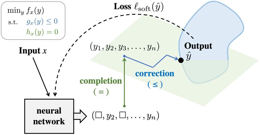
3 DC3: D EEP C ONSTRAINT C OMPLETION AND C ORRECTION
In this work, we consider solving families of optimization problems for which the objectives and/or
constraints vary across instances. Formally, let x ∈ Rd denote the problem data, and y ∈ Rn denote
the solution of the corresponding optimization problem (where y depends on x). For any given x,
our aim is then to find y solving:
minimize
n
fx (y), s. t. gx (y) ≤ 0, hx (y) = 0, (1)
y∈R
(where f , g, and h are potentially nonlinear and non-convex). Solving such a family of optimization
problems can be framed as a learning problem, where an algorithm must predict an optimal y from
the problem data x. We consider deep learning approaches to this task – that is, training a neural
network Nθ , parameterized by θ, to approximate y given x.
A naive deep learning approach to approximating such a problem involves viewing the constraints
as a form of regularization. That is, for training examples x(i) , the algorithm learns to minimize a
composite loss containing both the objective and two “soft loss” terms representing violations of the
equality and inequality constraints (for some λg , λh > 0):
`soft (ŷ) = fx (ŷ) + λg k ReLU(gx (ŷ))k22 + λh khx (ŷ)k22 . (2)
An alternative framework (see, e.g., Zamzam & Baker (2019)) is to use supervised learning on
examples (x(i) , y (i) ) for which an optimum y (i) is known. In this case, the loss is simply ||ŷ−y (i) ||22 .
However, both these procedures for training a neural network can lead in practice to highly infeasible
outputs (as we demonstrate in our experiments), because they do not strictly enforce constraints.
Supervised methods also require constructing a training set (e.g., via an exact solver), a sometimes
difficult or expensive step.
To address these challenges, we introduce the method of Deep Constraint Completion and Correc-
tion (DC3), which allows hard constraints to be integrated into the training of neural networks. This
method is able to train directly from the problem specification (instead of a supervised dataset), via
the following two innovations:
Equality completion. We provide a mechanism to enforce equality constraints during training and
testing, inspired by the literature on variable elimination. Specifically, rather than outputting the
full-dimensional optimization solution directly, we first output a subset of the variables, and then
infer the remaining variables via the equality constraints – either explicitly, or by solving an implicit
set of equations (through which we can then backpropagate via the implicit function theorem).
Inequality correction. We correct for violation of the inequality constraints by mapping infeasible
points to feasible points using an internal gradient descent procedure during training. This allows us
to fix inequality violations while taking steps along the manifold of points satisfying the equalities,
which yields an output that is feasible with respect to all constraints.
Overall, our algorithm involves training a neural network Nθ (x) to output a partial set of vari-
ables z. These variables are then completed to a full set of variables ỹ satisfying the equal-
ity constraints. In turn, ỹ is corrected to ŷ to satisfy the inequality constraints while contin-
uing to satisfy the equality constraints. The overall network is trained using backpropagation
on the soft loss described in Equation (2) (which is necessary for correction, as noted below).
Importantly, both the com-
pletion and correction pro-
cedures are differentiable ei-
ther implicitly or explicitly
(allowing network training to
take them into account), and
the overall framework is ag-
nostic to the choice of neu-
ral network architecture. A
schematic of the DC3 frame-
work is given in Figure 1, and
corresponding pseudocode is
given in Algorithm 1.
Figure 1: A schematic of the DC3 framework.
3Published as a conference paper at ICLR 2021
Algorithm 1 Deep Constraint Completion and Correction (DC3)
1: assume equality completion procedure ϕx : Rm → Rn−m // to solve equality constraints
2:
3: procedure TRAIN(X)
4: init neural network Nθ : Rd → Rm
5: while not converged do for x ∈ X
6: compute partial set of variables z = Nθ (x)
T
7: complete to full set of variables ỹ = z T ϕx (z)T ∈ Rn
(t )
8: correct to feasible (or approx. feasible) solution ŷ = ρx train (ỹ)
9: compute constraint-regularized loss `soft (ŷ)
10: update θ using ∇θ `soft (ŷ)
11: end while
12: end procedure
13:
14: procedure TEST(x, Nθ )
15: compute partial set of variables z = Nθ (x)
T
16: complete to full set of variables ỹ = z T ϕx (z)T
17: correct to feasible solution ŷ = ρ(ttest ) (ỹ)
18: return ŷ
19: end procedure
We note that as this procedure is somewhat general, in cases where constraints have a specialized
structure, specialized techniques may be more appropriate to use. For instance, while we examine
linearly-constrained settings in our experiments for the purposes of illustration, in practice, tech-
niques such as Minkowski-Weyl decomposition or Cholesky factorization (see Frerix et al. (2020),
Amos & Kolter (2017)) may be more efficient in these settings. However, for more general settings
without this kind of structure – e.g., non-convex problems such as AC optimal power flow, which
we examine in our experiments – the DC3 framework can provide a (differentiable) mechanism for
satisfying hard constraints. We now detail the completion and correction procedures used in DC3.
3.1 E QUALITY COMPLETION
Assuming that the problem (1) is not overdetermined, the number of equality constraints hx (y) = 0
must not exceed the dimension of the decision variable y ∈ Rn : that is, the number of equality
constraints equals n − m for some m ≥ 0. Then, given m of the entries of a feasible point y, the
other (n−m) entries are, in general, determined by the (n−m) equality constraints. We exploit this
observation in our algorithm, noting that it is considerably more efficient to output a point in Rm and
complete it to a point y ∈ Rn such that hx (y) = 0, as compared with outputting full-dimensional
points y ∈ Rn and attempting to adjust all coordinates to satisfy the equality constraints.
In particular, we assume that given m entries of y, we either can solve for the remaining entries ex-
plicitly (e.g. in a linear system) or that we have access to a process (e.g. Newton’s Method) allowing
us to solve any implicit equations. Formally, we assume access to a function ϕx : Rm → Rn−m
T T
such that hx ( z T ϕx (z)T ) = 0, where z T ϕx (z)T is the concatenation of z and ϕx (z).
In our algorithm, we then train our neural network Nθ to output points z ∈ Rm , which are completed
T
to z T ϕx (z)T ∈ Rn . A challenge then arises as to how to backpropagate the loss during
the training of Nθ if ϕx (z) is not a readily differentiable explicit function – for example, if the
completion procedure uses Newton’s Method. We solve this challenge by leveraging the implicit
function theorem, as e.g. in OptNet (Amos & Kolter, 2017) and SATNet (Wang et al., 2019). This
approach allows us to express, for any training loss `, the derivatives d`/dz using d`/dϕx (z).
Namely, let J h ∈ R(n−m)×n denote the Jacobian of hx (y) with respect to y. By the chain rule:
d z ∂hx ∂hx ∂ϕx (z) h h ∂ϕx (z)
0 = hx = + = J:,0:m + J:,m:n ,
dz ϕx (z) ∂z ∂ϕx (z) ∂z ∂z
h
−1 h
⇒ ∂ϕx (z)/∂z = − J:,m:n J:,0:m . (3)
4Published as a conference paper at ICLR 2021
We can then backpropagate losses through the network by noting that
d` ∂` ∂` ∂ϕx (z) ∂` ∂` −1 h
= + = − Jh J:,0:m . (4)
dz ∂z ∂ϕx (z) ∂z ∂z ∂ϕx (z) :,m:n
We note that in practice, the Jacobian ∂ϕx (z)/∂z should generally not be computed explicitly due to
space complexity considerations; instead, it is often desirable to form the result of the left matrix-
vector product (∂`/∂ϕx (z))(∂ϕx (z)/∂z) directly. This process is well-described in e.g. Amos & Kolter
(2017), and also in detail for the problem of AC optimal power flow in Appendix C.
3.2 I NEQUALITY CORRECTION
While the completion procedure described above guarantees feasibility with respect to the equality
constraints, it does not ensure that the inequality constraints will be satisfied. To additionally ensure
feasibility with respect to the inequality constraints, our algorithm incorporates a correction proce-
dure that maps the outputs from the previous step into the feasible region. In particular, we employ a
gradient-based correction procedure that takes gradient steps in z towards the feasible region along
the manifold of points satisfying the equality constraints.
T
Let ρx (y) be the operation that takes as input a point y = z T ϕx (z)T , and moves it closer to
satisfying the inequality constraints by taking a step along the gradient of the inequality violation
with respect to the partial variables z. Formally, for a learning rate γ > 0, we define:
z z − γ∆z
ρx = ,
ϕx (z) ϕx (z) − γ∆ϕx (z)
2
z ∂ϕx (z)
for ∆z = ∇z ReLU gx , ∆ϕx (z) = ∆z.
ϕx (z) 2 ∂z
While gradient descent methods do not always converge to global (or local) optima for general
optimization problems, if initialized close to an optimum, gradient descent is highly effective in
practice for non-pathological settings (see e.g. Busseti et al. (2019); Lee et al. (2017)). At test
time, the input to the DC3 correction procedure should already be close to feasible with respect to
the inequality constraints, as it is the output of a differentiable completion process that is trained
(t)
using the soft loss `soft . Therefore, we may expect that in practice, the limit limt→∞ ρx (y) will
converge to a point satisfying both inequality and equality constraints (while for problems with
linear constraints as in §4.1–4.2, the correction process is mathematically guaranteed to converge).
(t)
As the exact limit limt→∞ ρx (y) is difficult to calculate in practice, we make approximations at
(t)
both training and test time. Namely, we apply ρx (y) to the output of the completion procedure, with
t = ttrain relatively small at train time to allow backpropagation through the correction. Depending
on time constraints, this same value of t may be used at test time, or a larger value t = ttest > ttrain
may be used to ensure convergence to a feasible point.
4 E XPERIMENTS
We evaluate DC3 for convex quadratic programs (QPs), a simple family of non-convex optimization
problems, and the real-world task of AC optimal power flow (ACOPF). 1 In particular, we assess our
method on the following criteria:
• Optimality: How good is the objective value fx (y) achieved by the final solution?
• Feasibility: How much, if at all, does the solution violate the constraints? Specifically,
what are the maximum and mean feasibility violations of the inequality and equality con-
straints: max(ReLU(gx (y))), mean(ReLU(gx (y))), max(hx (y)), and mean(hx (y))?
• Speed: How fast is the method?
1
Code for all experiments is available at https://github.com/locuslab/DC3
5Published as a conference paper at ICLR 2021
We compare DC3 against the following methods (referred to by abbreviations in our tables below):
• Optimizer: A traditional optimization solver. For convex QP settings, we use OSQP (Stel-
lato et al., 2020), as well as the batched, differentiable solver qpth developed as part
of OptNet (Amos & Kolter, 2017). For the generic non-convex setting, we use IPOPT
(Wächter & Biegler, 2006). For ACOPF, we use the solver provided by PYPOWER, a
Python port of MATPOWER (Zimmerman et al., 1997).
• NN: A simple deep learning approach trained to minimize a soft loss (Equation (2)).
• NN, ≤ test: The NN approach, with a gradient-based correction procedure 2 applied to the
output at test time in an effort to mitigate violations of equality and inequality constraints.
Unlike in DC3, correction is not used during training, and completion is not used at all.
• Eq. NN: A more sophisticated approach inspired by 3 that in Zamzam & Baker (2019),
where (i) the neural network outputs a partial set of variables ẑ, which is completed to the
full set using the equality constraints, (ii) training is performed by supervised learning on
optimal pairs (x(i) , z (i) ) with loss function ||ẑ − z (i) ||22 , not using the objective value at all.
• Eq. NN, ≤ test: The approach in Eq. NN, augmented with gradient-based correction at test
time to mitigate violations of equality and inequality constraints.
We also attempted to use the output of the NN method as a “warm start” for traditional optimizers,
but found that the NN output was sufficiently far from feasibility that it did not help.
In addition, we consider weaker versions of DC3 in which components of the algorithm are ablated:
• DC3, 6=. The DC3 algorithm with completion ablated. All variables are output by the
network directly and correction is performed by taking gradient steps for both equality and
inequality constraints.
• DC3, 6≤ train. The DC3 algorithm with correction ablated at train time. Correction is still
performed at test time.
• DC3, 6≤ train/test. The DC3 algorithm with correction ablated at both train and test time.
• DC3, no soft loss. The DC3 algorithm with training performed to minimize the objective
value only, without auxiliary terms capturing equality and inequality violation.
As our overall framework is agnostic to the choice of neural network architecture, to facilitate com-
parison, we use a fixed neural network architecture across all experiments: fully connected with two
hidden layers of size 200, including ReLU activation, batch normalization, and dropout (with rate
0.2) at each hidden layer (Ioffe & Szegedy, 2015; Srivastava et al., 2014). For our correction proce-
dure, we use ttrain = ttest = 10 for the convex QP and simple non-convex tasks and ttrain = ttest = 5
for ACOPF (see Appendix B). All neural networks are trained using PyTorch (Paszke et al., 2019).
To generate timing results, all neural nets and the qpth optimizer were run with full paralleliza-
tion on a GeForce GTX 2080 Ti GPU. The OSQP, IPOPT, and PYPOWER optimizers were run
sequentially on an Intel Xeon 2.10GHz CPU, and we report the total time divided by the number of
test instances to simulate full parallelization. As our implementations are not tightly optimized, we
emphasize that all timing comparisons are approximate.
4.1 C ONVEX QUADRATIC PROGRAMS
As a first test of the DC3 method, we consider solving convex quadratic programs with a quadratic
objective function and linear constraints. Note that we examine this simple task first for illustration,
2
Note that this correction procedure is not exactly the same as that described in Section 3.2, as the outputs
of the NN baseline do not necessarily meet the prerequisite of satisfying the equality constraints. Instead, we
adjust the full set of output variables directly with respect to gradients of the inequality and equality violations.
3
In Zamzam & Baker (2019), the authors employ one step of an ACOPF-specific heuristic called PV/PQ
switching to correct inequality constraint violations at test time. We do not apply this heuristic here in the
spirit of presenting a more general framework. As PV/PQ switching is not necessarily guaranteed to correct
all inequality violations (although it can work well in practice), in principle, one could consider employing a
combination of PV/PQ switching and gradient-based corrections in the context of ACOPF.
6Published as a conference paper at ICLR 2021
Obj. value Max eq. Mean eq. Max ineq. Mean ineq. Time (s)
Optimizer (OSQP) -15.05 (0.00) 0.00 (0.00) 0.00 (0.00) 0.00 (0.00) 0.00 (0.00) 0.002 (0.000)
Optimizer (qpth) -15.05 (0.00) 0.00 (0.00) 0.00 (0.00) 0.00 (0.00) 0.00 (0.00) 1.335 (0.012)
DC3 -13.46 (0.01) 0.00 (0.00) 0.00 (0.00) 0.00 (0.00) 0.00 (0.00) 0.017 (0.001)
DC3, 6= -12.58 (0.04) 0.35 (0.00) 0.13 (0.00) 0.00 (0.00) 0.00 (0.00) 0.008 (0.000)
DC3, 6≤ train -1.39 (0.97) 0.00 (0.00) 0.00 (0.00) 0.02 (0.02) 0.00 (0.00) 0.017 (0.000)
DC3, 6≤ train/test -1.23 (1.21) 0.00 (0.00) 0.00 (0.00) 0.09 (0.13) 0.01 (0.01) 0.001 (0.000)
DC3, no soft loss -21.84 (0.00) 0.00 (0.00) 0.00 (0.00) 23.83 (0.11) 4.04 (0.01) 0.017 (0.000)
NN -12.57 (0.01) 0.35 (0.00) 0.13 (0.00) 0.00 (0.00) 0.00 (0.00) 0.001 (0.000)
NN, ≤ test -12.57 (0.01) 0.35 (0.00) 0.13 (0.00) 0.00 (0.00) 0.00 (0.00) 0.008 (0.000)
Eq. NN -9.16 (0.75) 0.00 (0.00) 0.00 (0.00) 8.83 (0.72) 0.91 (0.09) 0.001 (0.000)
Eq. NN, ≤ test -14.68 (0.05) 0.00 (0.00) 0.00 (0.00) 0.89 (0.05) 0.07 (0.01) 0.018 (0.001)
Table 1: Results on QP task for 100 variables, 50 equality constraints, and 50 inequality constraints.
We compare the performance of DC3 and other algorithms according to the objective value and
max/mean values of equality/inequality constraint violations, each averaged across test instances.
We also compare the total time required to run on all 833 test instances, assuming full parallelization.
(Std. deviations across 5 runs are shown in parentheses for all figures reported.) Lower values are
better for all metrics. We find that methods other than DC3 and Optimizer violate feasibility (as
shown in red). DC3 gives a feasible output with reasonable objective value 78× faster than qpth
and only 9× slower than OSQP, which is optimized for convex QPs.
but the general DC3 method is assuredly overkill for solving convex quadratic programs. It may not
even be the most efficient deep learning-based method for constraint enforcement on this task, since
more specialized techniques are available in such linearly constrained settings (Frerix et al., 2020).
We consider the following problem:
1 T
minimize y Qy + pT y, s. t. Ay = x, Gy ≤ h, (5)
n
y∈R 2
for constants Q ∈ Rn×n 0, p ∈ Rn , A ∈ Rneq ×n , G ∈ Rnineq ×n , h ∈ Rnineq , and variable x ∈ Rneq
which varies between problem instances. We must learn to approximate the optimal y given x.
In our experiments, we take Q to be a diagonal matrix with all diagonal entries drawn i.i.d. from
the uniform distribution on [0, 1], ensuring that Q is positive semi-definite. We take matrices A, G
with entries drawn i.i.d. from the unit normal distribution. We assume that in each problem instance,
P of x are in the interval [−1, 1]. In order to ensure that the problem is feasible, we take
all entries
h = j |(GA+ )ij |, where A+ is the Moore-Penrose pseudoinverse of A; namely, for this choice of
h, the point y = A+ x is feasible (but not, in general, optimal), because:
X
AA+ x = x, GA+ x ≤ (GA+ )ij since |xj | ≤ 1. (6)
j
During training, we use examples x with entries drawn i.i.d. from the uniform distribution on [−1, 1].
Table 1 compares the performance of DC3 (and various ablations of DC3) with traditional optimiz-
ers and other deep learning-based methods, for the case of n = 100 variables and neq = nineq = 50.
In Appendix A, we evaluate settings with other numbers of equality and inequality constraints. Each
experiment is run 5 times for 10,000 examples x (with train/test/validation ratio 10:1:1). Hyperpa-
rameters are tuned to maximize performance for each method individually (see Appendix B).
We find that DC3 preserves feasibility with respect to both equality and inequality constraints, while
achieving reasonable objective values. (The average per-instance optimality gap for DC3 over the
classical optimizer is 10.59%.) For every baseline deep learning algorithm, on the other hand,
feasibility is violated significantly for either equality or inequality constraints. As expected, “DC3
6=” (completion ablated) results in violated equality constraints, while “DC3 6≤” (correction ablated)
violates inequality constraints. Ablating the soft loss also results in violated inequality constraints,
leading to an objective value significantly lower than would be possible were constraints satisfied.
Even though we have not optimized the code of DC3 to be maximally fast, our implementation of
DC3 still runs about 78× faster than the state-of-the-art differentiable QP solver qpth, and only
7Published as a conference paper at ICLR 2021
Obj. value Max eq. Mean eq. Max ineq. Mean ineq. Time (s)
Optimizer -11.59 (0.00) 0.00 (0.00) 0.00 (0.00) 0.00 (0.00) 0.00 (0.00) 0.121 (0.000)
DC3 -10.66 (0.03) 0.00 (0.00) 0.00 (0.00) 0.00 (0.00) 0.00 (0.00) 0.013 (0.000)
DC3, 6= -10.04 (0.02) 0.35 (0.00) 0.13 (0.00) 0.00 (0.00) 0.00 (0.00) 0.009 (0.000)
DC3, 6≤ train -0.29 (0.67) 0.00 (0.00) 0.00 (0.00) 0.01 (0.01) 0.00 (0.00) 0.010 (0.004)
DC3, 6≤ train/test -0.27 (0.67) 0.00 (0.00) 0.00 (0.00) 0.03 (0.03) 0.00 (0.00) 0.001 (0.000)
DC3, no soft loss -13.81 (0.00) 0.00 (0.00) 0.00 (0.00) 15.21 (0.04) 2.33 (0.01) 0.013 (0.000)
NN -10.02 (0.01) 0.35 (0.00) 0.13 (0.00) 0.00 (0.00) 0.00 (0.00) 0.001 (0.000)
NN, ≤ test -10.02 (0.01) 0.35 (0.00) 0.13 (0.00) 0.00 (0.00) 0.00 (0.00) 0.009 (0.000)
Eq. NN -3.88 (0.56) 0.00 (0.00) 0.00 (0.00) 6.87 (0.43) 0.72 (0.05) 0.001 (0.000)
Eq. NN, ≤ test -10.99 (0.03) 0.00 (0.00) 0.00 (0.00) 0.87 (0.04) 0.06 (0.00) 0.013 (0.000)
Table 2: Results on our simple nonconvex task for 100 variables, 50 equality constraints, and 50
inequality constraints, with details as in Table 1. Since this problem is nonconvex, we use IPOPT
as the classical optimizer. DC3 is differentiable and about 9× faster than IPOPT, giving a near-
optimal objective value and constraint satisfaction, in contrast to baseline deep learning-based meth-
ods which result in significant constraint violations.
about 9× slower than the classical optimizer OSQP, which is specifically optimized for convex QPs.
Furthermore, this assumes OSQP is fully parallelized – in this case, across 833 CPUs – whereas
standard, non-parallel implementations of OSQP would be orders of magnitude slower. By contrast,
DC3 is easily parallelized within a single GPU using standard deep learning frameworks.
4.2 S IMPLE NON - CONVEX OPTIMIZATION
We now consider a simple non-convex adaptation of the quadratic program above:
1 T
minimize y Qy + pT sin(y), s. t. Ay = x, Gy ≤ h,
n
y∈R 2
where sin(y) denotes the componentwise application of the sine function to the vector y, and where
all constants and variables are defined as in (5). We consider instances of this problem where all
parameters are drawn randomly as in our preceding experiments in the convex setting.
In Table 2, we compare the performance of DC3 and other deep learning-based methods against the
classical non-convex optimizer IPOPT. 4 We find that DC3 achieves good objective values (8.02%
per-instance optimality gap), while maintaining feasibility. By contrast, all other deep learning-
based methods that we consider violate constraints significantly. DC3 also runs about 10× faster
than IPOPT, even assuming IPOPT is fully parallelized. (Even on the CPU, DC3 takes 0.030 ±
0.000 seconds, about 4× faster than IPOPT.) Note that the DC3 algorithm is essentially the same
between the convex QP and this non-convex task, since only the objective function is altered.
4.3 AC OPTIMAL POWER FLOW
We now show how DC3 can be applied to the problem of AC optimal power flow (ACOPF). ACOPF
is a fundamental problem for the operation of the electrical grid, and is used to determine how much
power must be produced by each generator on the grid in order to meet demand. As the amount of
renewable energy on the power grid grows, this problem must be solved more and more frequently to
account for the variability of these renewable sources, and at larger scale to account for an increasing
number of distributed devices (Rolnick et al., 2019). However, ACOPF is a non-convex optimization
problem and classical optimizers scale poorly on it. While specialized approaches to this problem
have started to emerge, including using machine learning (see, e.g., Zamzam & Baker (2019) for a
discussion), we here assess the ability of our more general framework to address this problem.
Formally, a power network may be considered as a graph on b nodes, representing different locations
(buses) within the electrical grid, and with edges weighted by complex numbers wij ∈ C (admit-
tances) that represent how easily current can flow between the corresponding locations in the grid.
Let W ∈ Cb×b denote the graph Laplacian (or nodal admittance matrix). Then, the problem of
ACOPF can be defined as follows: Given input variables pd ∈ Rb , qd ∈ Rb (representing real power
4
We initialize the optimizer using the feasible point y = A+ x noted in Equation (6).
8Published as a conference paper at ICLR 2021
Obj. value Max eq. Mean eq. Max ineq. Mean ineq. Time (s)
Optimizer 3.81 (0.00) 0.00 (0.00) 0.00 (0.00) 0.00 (0.00) 0.00 (0.00) 0.949 (0.002)
DC3 3.82 (0.00) 0.00 (0.00) 0.00 (0.00) 0.00 (0.00) 0.00 (0.00) 0.089 (0.000)
DC3, 6= 3.67 (0.01) 0.14 (0.01) 0.02 (0.00) 0.00 (0.00) 0.00 (0.00) 0.040 (0.000)
DC3, 6≤ train 3.82 (0.00) 0.00 (0.00) 0.00 (0.00) 0.00 (0.00) 0.00 (0.00) 0.089 (0.000)
DC3, 6≤ train/test 3.82 (0.00) 0.00 (0.00) 0.00 (0.00) 0.01 (0.00) 0.00 (0.00) 0.039 (0.000)
DC3, no soft loss 3.11 (0.05) 2.60 (0.35) 0.07 (0.00) 2.33 (0.33) 0.03 (0.01) 0.088 (0.000)
NN 3.69 (0.02) 0.19 (0.01) 0.03 (0.00) 0.00 (0.00) 0.00 (0.00) 0.001 (0.000)
NN, ≤ test 3.69 (0.02) 0.16 (0.00) 0.02 (0.00) 0.00 (0.00) 0.00 (0.00) 0.040 (0.000)
Eq. NN 3.81 (0.00) 0.00 (0.00) 0.00 (0.00) 0.15 (0.01) 0.00 (0.00) 0.039 (0.000)
Eq. NN, ≤ test 3.81 (0.00) 0.00 (0.00) 0.00 (0.00) 0.15 (0.01) 0.00 (0.00) 0.078 (0.000)
Table 3: Results on ACOPF over 100 test instances. We compare the performance of DC3 and
other algorithms according to the metrics described in Table 1. We find again that baseline methods
violate feasibility (as shown in red), while DC3 gives a feasible and near-optimal output about 10×
faster than the PYPOWER optimizer, even assuming that PYPOWER is fully parallelized.
and reactive power demand at the various nodes of the graph), output the variables pg ∈ Rb , qg ∈ Rb
(representing real power and reactive power generation) and v ∈ Cb (representing real and imagi-
nary voltage), according to the following optimization problem:
minimize pTg Apg + bT pg
pg ∈Rb , qg ∈Rb , v∈Cb
subject to pmin ≤ pg ≤ pmax , qgmin ≤ qg ≤ qgmax , v min ≤ |v| ≤ v max , (7)
g g
(pg − pd ) + (qg − qd )i = diag(v)W v.
More details about how we apply DC3 to the problem of ACOPF are given in Appendix C.
We assess our method on a 57-node power system test case available via the MATPOWER package.
We conduct 5 runs over 1,200 input datapoints (with a train/test/validation ratio of 10:1:1). As with
other tasks, hyperparameters for ACOPF were tuned to maximize performance for each method
individually (see Appendix B). Optimality, feasibility, and timing results are reported in Table 3.
We find that DC3 achieves comparable objective values to the optimizer, and preserves feasibility
with respect to both equality and inequality constraints. Once again, for every baseline deep learning
algorithm, feasibility is violated significantly for either equality or inequality constraints. Ablations
of DC3 also suffer from constraint violations, though the effect is less pronounced than for the con-
vex QP and simple non-convex settings, especially for ablation of the correction (perhaps because
the inequality constraints here are easier to satisfy than the equality constraints). We also see that
DC3 runs about 10× faster than the PYPOWER optimizer, even when PYPOWER is fully parallelized.
(Even when running on the CPU, DC3 takes 0.906 ± 0.003 seconds, slightly faster than PYPOWER.)
Out of 100 test instances, there were 3 on which DC3 output lower-than-optimal objective values of
up to a few percent (-0.30%, -1.85%, -5.51%), reflecting slight constraint violations. Over the other
97 instances, the per-instance optimality gap compared to the classical optimizer was 0.22%.
5 C ONCLUSION
We have described a method, DC3, for fast approximate solutions to optimization problems with
hard constraints. Our approach includes a neural network that outputs a partial set of variables,
a differentiable completion procedure that fills in remaining variables according to equality con-
straints, and a differentiable correction procedure that fixes inequality violations. We find that DC3
yields solutions of significantly better feasibility and objective value than other approximate deep
learning-based solvers on convex and non-convex optimization tasks.
We note that, while DC3 provides a general framework for tackling constrained optimization, de-
pending on the setting, the expensiveness of both the completion and correction procedures may
vary (e.g., implicit solutions may be more time-consuming, or gradient descent may converge more
or less easily). We believe that, while our method as stated is broadly applicable, it will be possible
in future work to design further improvements tailored to specific problem instances, for example
by designing problem-dependent correction procedures.
9Published as a conference paper at ICLR 2021
ACKNOWLEDGMENTS
This work was supported by the U.S. Department of Energy Computational Science Graduate Fel-
lowship (DE-FG02-97ER25308), U.S. National Science Foundation (DMS-1803547), the Center
for Climate and Energy Decision Making through a cooperative agreement between the National
Science Foundation and Carnegie Mellon University (SES-00949710), the Computational Sustain-
ability Network, and the Bosch Center for AI.
We thank Shaojie Bai, Rizal Fathony, Filipe de Avila Belbute Peres, Josh Williams, and anonymous
reviewers for their feedback on this work.
R EFERENCES
Akshay Agrawal, Brandon Amos, Shane Barratt, Stephen Boyd, Steven Diamond, and J Zico Kolter.
Differentiable convex optimization layers. In Advances in Neural Information Processing Systems
(NeurIPS), 2019.
Brandon Amos. Differentiable optimization-based modeling for machine learning. PhD thesis,
Carnegie Mellon University, 2019.
Brandon Amos and J Zico Kolter. OptNet: Differentiable optimization as a layer in neural networks.
In International Conference on Machine Learning (ICML), 2017.
Shaojie Bai, J Zico Kolter, and Vladlen Koltun. Deep equilibrium models. In Advances in Neural
Information Processing Systems (NeurIPS), 2019.
Kyri Baker. Learning warm-start points for AC optimal power flow. In 2019 IEEE 29th International
Workshop on Machine Learning for Signal Processing (MLSP), pp. 1–6, 2019.
Yoshua Bengio, Andrea Lodi, and Antoine Prouvost. Machine learning for combinatorial optimiza-
tion: a methodological tour d’horizon. European Journal of Operational Research, 2020.
Tom Beucler, Stephan Rasp, Michael Pritchard, and Pierre Gentine. Achieving conservation of
energy in neural network emulators for climate modeling. Preprint arXiv:1906.06622, 2019.
Enzo Busseti, Walaa M Moursi, and Stephen Boyd. Solution refinement at regular points of conic
problems. Computational Optimization and Applications, 74(3):627–643, 2019.
Ricky TQ Chen, Yulia Rubanova, Jesse Bettencourt, and David K Duvenaud. Neural ordinary
differential equations. In Advances in Neural Information Processing Systems (NeurIPS), 2018.
Taco Cohen and Max Welling. Group equivariant convolutional networks. In International Confer-
ence on Machine Learning (ICML), 2016.
Filipe de Avila Belbute-Peres, Kevin Smith, Kelsey Allen, Josh Tenenbaum, and J Zico Kolter.
End-to-end differentiable physics for learning and control. In Advances in Neural Information
Processing Systems (NeurIPS), 2018.
Josip Djolonga and Andreas Krause. Differentiable learning of submodular models. In Advances in
Neural Information Processing Systems (NeurIPS), 2017.
Wenqian Dong, Zhen Xie, Gokcen Kestor, and Dong Li. Smart-PGSim: Using neural network to
accelerate AC-OPF power grid simulation. arXiv preprint arXiv:2008.11827, 2020.
Priya L Donti, Brandon Amos, and J Zico Kolter. Task-based end-to-end model learning in stochastic
optimization. Preprint arXiv:1703.04529, 2017.
Thomas Frerix, Matthias Nießner, and Daniel Cremers. Homogeneous linear inequality constraints
for neural network activations. In Proceedings of the IEEE/CVF Conference on Computer Vision
and Pattern Recognition Workshops, pp. 748–749, 2020.
Stephen Gould, Richard Hartley, and Dylan Campbell. Deep declarative networks: A new hope.
Preprint arXiv:1909.04866, 2019.
10Published as a conference paper at ICLR 2021
Samuel Greydanus, Misko Dzamba, and Jason Yosinski. Hamiltonian neural networks. In Advances
in Neural Information Processing Systems (NeurIPS), 2019.
Fouad Hasan, Amin Kargarian, and Ali Mohammadi. A survey on applications of machine learning
for optimal power flow. In 2020 IEEE Texas Power and Energy Conference (TPEC), pp. 1–6.
IEEE, 2020.
Sergey Ioffe and Christian Szegedy. Batch normalization: Accelerating deep network training by
reducing internal covariate shift. In International Conference on Machine Learning (ICML), 2015.
Slawomir Koziel and Leifur Leifsson. Surrogate-based modeling and optimization. Springer, 2013.
Jason D Lee, Ioannis Panageas, Georgios Piliouras, Max Simchowitz, Michael I Jordan, and Ben-
jamin Recht. First-order methods almost always avoid saddle points. Preprint arXiv:1710.07406,
2017.
Chun Kai Ling, Fei Fang, and J Zico Kolter. What game are we playing? End-to-end learning in
normal and extensive form games. Preprint arXiv:1805.02777, 2018.
Sidhant Misra, Line Roald, and Yeesian Ng. Learning for constrained optimization: Identifying
optimal active constraint sets. Preprint arXiv:1802.09639, 2018.
Jorge Nocedal and Stephen Wright. Numerical optimization. Springer Science & Business Media,
2006.
Adam Paszke, Sam Gross, Francisco Massa, Adam Lerer, James Bradbury, Gregory Chanan, Trevor
Killeen, Zeming Lin, Natalia Gimelshein, Luca Antiga, et al. PyTorch: An imperative style,
high-performance deep learning library. In Advances in Neural Information Processing Systems
(NeurIPS), 2019.
David Rolnick, Priya L Donti, Lynn H Kaack, Kelly Kochanski, Alexandre Lacoste, Kris Sankaran,
Andrew Slavin Ross, Nikola Milojevic-Dupont, Natasha Jaques, Anna Waldman-Brown, et al.
Tackling climate change with machine learning. Preprint arXiv:1906.05433, 2019.
Nitish Srivastava, Geoffrey Hinton, Alex Krizhevsky, Ilya Sutskever, and Ruslan Salakhutdinov.
Dropout: a simple way to prevent neural networks from overfitting. Journal of Machine Learning
Research, 15(1):1929–1958, 2014.
B. Stellato, G. Banjac, P. Goulart, A. Bemporad, and S. Boyd. OSQP: an operator splitting solver
for quadratic programs. Mathematical Programming Computation, 12(4):637–672, 2020.
Sebastian Tschiatschek, Aytunc Sahin, and Andreas Krause. Differentiable submodular maximiza-
tion. Preprint arXiv:1803.01785, 2018.
Andreas Wächter and Lorenz T Biegler. On the implementation of an interior-point filter line-
search algorithm for large-scale nonlinear programming. Mathematical programming, 106(1):
25–57, 2006.
Po-Wei Wang, Priya L Donti, Bryan Wilder, and Zico Kolter. SATNet: Bridging deep learning
and logical reasoning using a differentiable satisfiability solver. In International Conference on
Machine Learning (ICML), 2019.
Bryan Wilder, Bistra Dilkina, and Milind Tambe. Melding the data-decisions pipeline: Decision-
focused learning for combinatorial optimization. In AAAI Conference on Artificial Intelligence,
2018.
Ahmed Zamzam and Kyri Baker. Learning optimal solutions for extremely fast AC optimal power
flow. Preprint arXiv:1910.01213, 2019.
Ray D Zimmerman, Carlos E Murillo-Sánchez, and Deqiang Gan. MATPOWER: A MATLAB
power system simulation package. Manual, Power Systems Engineering Research Center, Ithaca
NY, 1, 1997.
11Published as a conference paper at ICLR 2021
Optimizers Obj. val. -27.26 (0.00) -23.13 (0.00) -15.05 (0.00) -14.80 (0.00) -4.79 (0.00)
Max eq. 0.00 (0.00) 0.00 (0.00) 0.00 (0.00) 0.00 (0.00) 0.00 (0.00)
(OSQP, qpth)
Max ineq. 0.00 (0.00) 0.00 (0.00) 0.00 (0.00) 0.00 (0.00) 0.00 (0.00)
Obj. val. -25.79 (0.02) -20.29 (0.20) -13.46 (0.01) -13.73 (0.02) -4.76 (0.00)
DC3 Max eq. 0.00 (0.00) 0.00 (0.00) 0.00 (0.00) 0.00 (0.00) 0.00 (0.00)
Max ineq. 0.00 (0.00) 0.00 (0.00) 0.00 (0.00) 0.00 (0.00) 0.00 (0.00)
Obj. val. -22.59 (0.18) -20.40 (0.03) -12.58 (0.04) -13.36 (0.02) -5.27 (0.00)
DC3, 6= Max eq. 0.12 (0.01) 0.24 (0.00) 0.35 (0.00) 0.47 (0.00) 0.59 (0.00)
Max ineq. 0.00 (0.00) 0.00 (0.00) 0.00 (0.00) 0.00 (0.00) 0.00 (0.00)
Obj. val. -25.75 (0.04) -20.14 (0.15) -1.39 (0.97) -13.71 (0.04) -4.75 (0.00)
DC3, 6≤ train Max eq. 0.00 (0.00) 0.00 (0.00) 0.00 (0.00) 0.00 (0.00) 0.00 (0.00)
Max ineq. 0.00 (0.00) 0.00 (0.00) 0.02 (0.02) 0.00 (0.00) 0.00 (0.00)
Obj. val. -25.75 (0.04) -20.14 (0.15) -1.23 (1.21) -13.71 (0.04) -4.75 (0.00)
DC3, 6≤ train/test Max eq. 0.00 (0.00) 0.00 (0.00) 0.00 (0.00) 0.00 (0.00) 0.00 (0.00)
Max ineq. 0.00 (0.00) 0.00 (0.00) 0.09 (0.13) 0.00 (0.00) 0.00 (0.00)
Obj. val. -66.79 (0.01) -40.63 (0.02) -21.84 (0.00) -15.56 (0.02) -4.76 (0.01)
DC3, no soft loss Max eq. 0.00 (0.00) 0.00 (0.00) 0.00 (0.00) 0.00 (0.00) 0.00 (0.00)
Max ineq. 122.52 (0.22) 50.25 (0.14) 23.83 (0.11) 5.85 (0.18) 0.00 (0.00)
Obj. val. -22.65 (0.12) -20.43 (0.03) -12.57 (0.01) -13.35 (0.03) -5.29 (0.02)
NN Max eq. 0.11 (0.01) 0.24 (0.00) 0.35 (0.00) 0.47 (0.00) 0.59 (0.00)
Max ineq. 0.00 (0.00) 0.00 (0.00) 0.00 (0.00) 0.00 (0.00) 0.00 (0.00)
Obj. val. -22.65 (0.12) -20.43 (0.03) -12.57 (0.01) -13.35 (0.03) -5.29 (0.02)
NN, ≤ test Max eq. 0.11 (0.01) 0.24 (0.00) 0.35 (0.00) 0.47 (0.00) 0.59 (0.00)
Max ineq. 0.00 (0.00) 0.00 (0.00) 0.00 (0.00) 0.00 (0.00) 0.00 (0.00)
Obj. val. -27.20 (0.02) -22.74 (0.14) -9.16 (0.75) -14.64 (0.01) -4.74 (0.01)
Eq. NN Max eq. 0.00 (0.00) 0.00 (0.00) 0.00 (0.00) 0.00 (0.00) 0.00 (0.00)
Max ineq. 0.43 (0.02) 1.37 (0.09) 8.83 (0.72) 0.86 (0.05) 0.00 (0.00)
Obj. val. -27.20 (0.02) -22.76 (0.13) -14.68 (0.05) -14.65 (0.01) -4.74 (0.01)
Eq. NN, ≤ test Max eq. 0.00 (0.00) 0.00 (0.00) 0.00 (0.00) 0.00 (0.00) 0.00 (0.00)
Max ineq. 0.42 (0.02) 1.27 (0.09) 0.89 (0.05) 0.85 (0.05) 0.00 (0.00)
Table A.1: Results on QP task for 100 variables and 50 inequality constraints, as the number of
equality constraints varies as 10, 30, 50, 70, 90. We compare the performance of DC3 and other
algorithms according to objective value and maximum equality/inequality constraint violations av-
eraged across test instances. (Standard deviations across 5 runs are shown in parentheses.) We
find that neural network baselines give significantly inferior performance (shown in red) across all
problems.
A A DDITIONAL QP TASK RESULTS
We compare the performance of DC3 against other methods for the convex QP task with 100 vari-
ables, as the number of equality constraints (Table A.1) and inequality constraints (Table A.2) varies.
B D ETAILS ON HYPERPARAMETER TUNING
The following parameters were kept fixed for all neural network-based methods across all exper-
iments, based on a small amount of informal experimentation to ensure training was stable and
properly converged:
• Epochs: 1000
• Batch size: 5 200
• Hidden layer size: 200 (for both hidden layers)
• Correction procedure stopping tolerance: 10−4
• Correction procedure momentum: 0.5
5
While this batch size was used for training, final timing experiments were run with all test datapoints in
one batch.
12Published as a conference paper at ICLR 2021
10 30 50 70 90
Optimizers Obj. val. -17.33 (0.00) -16.33 (0.00) -15.05 (0.00) -14.61 (0.00) -14.26 (0.00)
Max eq. 0.00 (0.00) 0.00 (0.00) 0.00 (0.00) 0.00 (0.00) 0.00 (0.00)
(OSQP, qpth)
Max ineq. 0.00 (0.00) 0.00 (0.00) 0.00 (0.00) 0.00 (0.00) 0.00 (0.00)
Obj. val. -15.18 (0.31) -13.90 (0.20) -13.46 (0.01) -10.52 (0.93) -11.77 (0.07)
DC3 Max eq. 0.00 (0.00) 0.00 (0.00) 0.00 (0.00) 0.00 (0.00) 0.00 (0.00)
Max ineq. 0.00 (0.00) 0.00 (0.00) 0.00 (0.00) 0.00 (0.00) 0.00 (0.00)
Obj. val. -15.66 (0.05) -14.10 (0.04) -12.58 (0.04) -12.10 (0.03) -11.72 (0.03)
DC3, 6= Max eq. 0.35 (0.00) 0.35 (0.00) 0.35 (0.00) 0.35 (0.00) 0.35 (0.00)
Max ineq. 0.00 (0.00) 0.00 (0.00) 0.00 (0.00) 0.00 (0.00) 0.00 (0.00)
Obj. val. -15.60 (0.30) -13.83 (0.15) -1.39 (0.97) -11.14 (0.05) -11.76 (0.06)
DC3, 6≤ train Max eq. 0.00 (0.00) 0.00 (0.00) 0.00 (0.00) 0.00 (0.00) 0.00 (0.00)
Max ineq. 0.00 (0.00) 0.00 (0.00) 0.02 (0.02) 0.00 (0.00) 0.00 (0.00)
Obj. val. -15.60 (0.30) -13.83 (0.15) -1.23 (1.21) -11.14 (0.05) -11.76 (0.06)
DC3, 6≤ train/test Max eq. 0.00 (0.00) 0.00 (0.00) 0.00 (0.00) 0.00 (0.00) 0.00 (0.00)
Max ineq. 0.00 (0.00) 0.00 (0.00) 0.09 (0.13) 0.00 (0.00) 0.00 (0.00)
Obj. val. -21.78 (0.01) -21.72 (0.03) -21.84 (0.00) -21.82 (0.01) -21.83 (0.00)
DC3, no soft loss Max eq. 0.00 (0.00) 0.00 (0.00) 0.00 (0.00) 0.00 (0.00) 0.00 (0.00)
Max ineq. 23.85 (0.52) 23.54 (0.23) 23.83 (0.11) 23.73 (0.09) 23.69 (0.06)
Obj. val. -15.66 (0.03) -14.10 (0.05) -12.57 (0.01) -12.12 (0.03) -11.70 (0.02)
NN Max eq. 0.35 (0.00) 0.35 (0.00) 0.35 (0.00) 0.35 (0.00) 0.35 (0.00)
Max ineq. 0.00 (0.00) 0.00 (0.00) 0.00 (0.00) 0.00 (0.00) 0.00 (0.00)
Obj. val. -15.66 (0.03) -14.10 (0.05) -12.57 (0.01) -12.12 (0.03) -11.70 (0.02)
NN, ≤ test Max eq. 0.35 (0.00) 0.35 (0.00) 0.35 (0.00) 0.35 (0.00) 0.35 (0.00)
Max ineq. 0.00 (0.00) 0.00 (0.00) 0.00 (0.00) 0.00 (0.00) 0.00 (0.00)
Obj. val. -17.07 (0.20) -15.45 (0.09) -9.16 (0.75) -14.20 (0.06) -14.10 (0.10)
Eq. NN Max eq. 0.00 (0.00) 0.00 (0.00) 0.00 (0.00) 0.00 (0.00) 0.00 (0.00)
Max ineq. 1.65 (0.22) 1.79 (0.10) 8.83 (0.72) 2.26 (0.04) 1.28 (0.05)
Obj. val. -17.06 (0.20) -15.65 (0.09) -14.68 (0.05) -14.31 (0.06) -14.10 (0.10)
Eq. NN, ≤ test Max eq. 0.00 (0.00) 0.00 (0.00) 0.00 (0.00) 0.00 (0.00) 0.00 (0.00)
Max ineq. 1.53 (0.19) 1.58 (0.08) 0.89 (0.05) 1.92 (0.04) 1.25 (0.04)
Table A.2: Results on QP task for 100 variables and 50 equality constraints. The number of inequal-
ity constraints varies as 10, 30, 50, 70, 90. Content and interpretation as in Table A.1.
For all remaining parameters, we performed hyperparameter tuning via a coordinate search over
relevant parameters. Central values for this coordinate search were determined via a small amount
of informal experimentation to ensure training was stable on that central set of parameters. Final
parameters were chosen so as to prioritize feasibility (as determined via the mean and max violations
of equality and inequality constraints), followed by objective value and speed.
B.1 C ONVEX QUADRATIC PROGRAMS
We list the ranges over which different hyperparameters were tuned for each method, with central
values for the coordinate search in italics, and the final parameter values in bold. In order to min-
imize the amount of tuning, we employ the hyperparameters obtained for DC3 to “DC3, 6≤ train”
and “DC3, no soft loss” as well (rather than tuning the latter two methods separately). For this set
of experiments, we set the learning rate of the gradient-based correction procedure ρx to 10−7 for
all methods, as most methods went unstable for higher correction learning rates.
DC3
DC3, 6≤ train DC3, 6= NN Eq. NN
DC3, no soft loss
Lr 10−2 , 10 −3 , 10−4 10−2 , 10 −3 , 10−4 10−2 , 10 −3 , 10−4 10−2 , 10 −3 , 10−4
λg + λh 1,10,100 1,10,100 1,10,100 –
λh
λg +λh 0.5, 0.1, 0.01 0.5, 0.9, 0.99 0.5, 0.9, 0.99 –
ttest 5, 10, 50, 100, 1000 5, 10, 50, 100, 1000 5, 10, 50, 100, 1000 5, 10, 50, 100, 1000
ttrain 1, 2, 5, 10, 100 1, 2, 5, 10, 100 – –
13Published as a conference paper at ICLR 2021
B.2 S IMPLE NON - CONVEX OPTIMIZATION
All hyperparameters in these experiments were maintained at the settings chosen for the convex QP
task, since these tasks were similar by design.
B.3 AC OPTIMAL POWER FLOW
We list the ranges over which different hyperparameters were tuned for each method, with central
values for the coordinate search in italics, and the final parameter values in bold. As in the previous
setting, in order to minimize the amount of tuning, we employ the hyperparameters obtained for
DC3 to “DC3, 6≤ train” and “DC3, no soft loss” as well (rather than tuning the latter two methods
separately).
DC3
DC3, 6≤ train DC3, 6= NN Eq. NN
DC3, no soft loss
Lr 10−2 , 10 −3 , 10−4 10−2 , 10 −3 , 10−4 10−2 , 10 −3 , 10−4 10−2 , 10 −3 , 10−4
λg + λh 1,10,100 1,10,100 1,10,100 –
λh
λg +λh 0.5, 0.1, 0.01 0.5, 0.9, 0.99 0.5, 0.9, 0.99 –
ttest 5, 10, 50, 100 5, 10, 50, 100 5, 10, 50, 100 5, 10, 50, 100, 200
ttrain 1, 2, 5, 10, 100 1, 2, 5, 10, 100 – –
Lr, ρx 10−3 , 10 −4 , 10−5 10−4 , 10 −5 , 10−6 10−5 , 10 −6 , 10−7 10−5 , 10 −6 , 10−7
C D ETAILS OF DC3 FOR ACOPF
C.1 P ROBLEM SETTING
We consider the problem of ACOPF defined in §4.3.
Let B denote the overall set of buses (i.e., nodes in the power network). In any instance of ACOPF
there exists a set D ⊆ B of load (demand) buses at which pg and qg are identically zero, as well as
a set R ⊆ B of reference (slack) buses at which pg and qg are potentially nonzero, and where the
voltage angle ∠v is known. Let G = B \ (D ∪ R) be the remaining generator buses at which pg and
qg are potentially nonzero, but where the voltage angle ∠v is not known.
Then, we may rewrite Equation (7) as follows, where v ≡ |v|ei∠v and W ≡ Wr + Wi i:
minimize pTg Apg + bT pg (C.1a)
pg ,qg ,|v|,∠v∈R|B|
subject to pmin
g ≤ pg ≤ pmax
g (C.1b)
qgmin ≤ qg ≤ qgmax (C.1c)
min max
v ≤ |v| ≤ v (C.1d)
(∠v)R = φslack (C.1e)
(pg )D = (qg )D = 0 (C.1f)
pg − pd − diag(vr )(Wr vr − Wi vi ) − diag(vi )(Wi vr + Wr vi ) = 0 (C.1g)
qg − qd + diag(vr )(Wi vr + Wr vi ) − diag(vi )(Wr vr − Wi vi ) = 0 (C.1h)
where vr = |v| cos(∠v) and vi = |v| sin(∠v)
(While we write the problem in this form to minimize notation, in practice, some of the constraints
in the above problem – e.g., (C.1b), (C.1c), and (C.1f) – can be condensed.)
C.2 OVERALL APPROACH
As pointed out in Zamzam & Baker (2019), given pd , qd , (pg )G and |v|B\D , the remaining variables
(pg )R , (qg )B\D , |v|D , and (∠v)B\R can be recovered via the power flow equations (C.1g)–(C.1h).
14Published as a conference paper at ICLR 2021
As such, our implementation of DC3 may be outlined as follows.
T
• Input: x = pTd qdT . (The constant ∠vR is fixed across problem instances.)
• Neural network: Output α ∈ [0, 1]|G| and β ∈ [0, 1]|B|−|D| (applying a sigmoid to the
final layer of the network), and compute:
(pg )G = α(pmin max
g )G + (1 − α)(pg )G ,
min max
|v|B\D = βvB\D + (1 − β)vB\D .
(In other words, output a partial set of variables, and enforce box constraints on this set of
variables via sigmoids in the neural network.)
h iT
• Completion procedure: Given z = (pg )TG |v|TB\D , solve Equations (C.1g)–(C.1h)
for the remaining quantities (pg )R , (qg )B\D , |v|D , and (∠v)B\R as described below. Out-
T
put all decision variables y = (pg )TG (qg )TG |v|T (∠v)T .
• Correction procedure: Correct y using the gradient-based feasibility correction procedure
described in §3.2.
• Backpropagate: Compute the loss and backpropagate as described below to update neural
network parameters. Repeat until convergence.
We now describe the forward and backward passes through the completion procedure, where we
have introduced several “tricks” that significantly reduce the computational cost, including some
that are specific to the ACOPF setting.
For ease of notation throughout, we will let J ∈ R1+2|B| denote the Jacobian of the equality con-
straints (C.1e)–(C.1h) with respect to the complete vector y of decision variables. This matrix, which
we pre-compute, will be useful throughout our computations.
C.3 S OLVING THE COMPLETION
The neural network outputs (pg )G and |v|B\D are the inputs to the completion procedure. The-
oretically, we could use Newton’s method to solve for all additional variables from the equality
constraints. However, in practice we find that solving for all variables using Newton’s method is
sometimes unstable. Fortunately, we can divide the completion procedure into two substeps, where
Step 1 invokes Newton’s method to identify some of the variables, while Step 2 solves in closed
form for the others. This greatly improves the stability of the completion procedure.
Step 1. Compute |v|D , (∠v)B\R via Newton’s method using real power flow constraints (C.1g) at
buses B \ R, and reactive power constraints (C.1h) at buses D (note that the number of equations
matches the number of variables being identified). We initialize Newton’s method by fixing variables
determined by the neural network and those already determined in Step 1 of the completion process,
and initializing |v|D , (∠v)B\R at generic initial values (these are provided in the ACOPF task setup
and are typically used to initialize state-of-the-art solvers). Note that the remaining variables, those
determined in Step 2 of the completion process, do not actually appear in the relevant equality
constraints and therefore do not need to be set.
Let J Step 1 denote the submatrix of J corresponding to the equality constraints (C.1g)B\R and
(C.1h)D and the voltage variables |v|D and (∠v)B\R that we are solving in this step. At the tth
step of Newton’s method, let h Step 1 (t) ∈ R|B|−|R|+|D| denote the vector of values on the left-hand
side of the relevant equality constraints (which we wish to equal identically zero), evaluated at the
current setting of all problem variables. Our Newton’s method updates are then
" # " #
|v|D |v|D
= − J −1
Step 1 h Step 1 (t). (C.2)
(∠v)B\R (∠v)B\R
t+1 t
15You can also read