Energy Consumption, Economic Growth And Environmental Sustainability Challenges For Belt And Road Countries: A Fresh Insight From "Chinese Going ...

Energy Consumption, Economic Growth And
Environmental Sustainability Challenges For Belt
And Road Countries: A Fresh Insight From “Chinese
Going Global Strategy”
Abdul Jalil (  jalil_ahmed21@yahoo.com )
 Nanjing University of Information Science and Technology Binjiang College https://orcid.org/0000-
0002-4317-8226
Abdul Rauf
 Nanjing University of Information Science and Technology
Waqas Sikander
 University of the Punjab Quaid-i-Azam Campus: University of the Punjab
Zhang Yonghong
 Nanjing University of Information Science and Technology Binjiang College
Wang Tiebang
 Nanjing University of Information Science and Technology Binjiang College

Research Article

Keywords: Energy consumption, Economy, Environment, Belt and Road Initiative, Sustainable
development, Carbon Dioxide

Posted Date: June 15th, 2021

DOI: https://doi.org/10.21203/rs.3.rs-573704/v1

License:   This work is licensed under a Creative Commons Attribution 4.0 International License.
Read Full License

Version of Record: A version of this preprint was published at Environmental Science and Pollution
Research on July 29th, 2021. See the published version at https://doi.org/10.1007/s11356-021-15549-z.

1

 1 Energy consumption, Economic growth and Environmental Sustainability

 2 Challenges for Belt and Road Countries: A Fresh Insight from “Chinese

 3 Going Global Strategy”

 4

 5 Abdul Jalila*, Abdul Raufb**, Waqas Sikanderc, Zhang Yonghonga, Wang Tiebanga

 6

 a
 7 Binjiang College, Nanjing University of Information Science and Technology, 333, Xishan road,
 8 Wuxi, 214105, China

 b
 9 School of Management Science and Engineering, Nanjing University of Information Science
10 and Technology, Nanjing, 210044, China

 c
11 College of Earth and Environmental Science, University of the Punjab, New Quaid-e-Azam
12 campus, Lahore, Pakistan

13 Corresponding Authors:
14 *Abdul Jalil
15 Binjiang College, Nanjing University of Information Science and Technology, No 333, Xishan
16 road, Wuxi city, Jiangsu, 214105, China
17 Tel: +86-15905173417
18 E-mail: jalil_ahmed21@hotmail.com
19 **Abdul Rauf
20 School of Management and Engineering, Nanjing University of Information Science and
21 Technology, 219, Ningliu Road, Nanjing, Jiangsu, 210044, China
22 Tel: +86-13770641422
23 E-mail: abdulrauf@seu.edu.cn

2

24 Abstract

25 The present study investigated impact of energy and economy related variables on CO2

26 emissions in 49 countries of belt and road initiative from 1995-2018. The robust type of cross-

27 section dependence and heterogeneity methods were adopted to analyze data set of countries.

28 Energy consumption, foreign direct investment, medium and high-tech industry, and GDP has

29 been found highly unfavorable for the ecological health (CO2 emissions) in 49 nations on BRI

30 panel. However, renewable energy consumption has been found in positive correlation with

31 environmental quality (CO2). Financial development indicator has no significant impact on CO2

32 emissions in present study. The present outcomes clearly claim strong relationship of economic

33 growth and energy with increased CO2 emissions in 49 nations. Therefore, it is important for

34 policy makers, experts and governments to incentivize and appreciate portfolio investors for

35 sustainable green investments to transform the economic growth into a sustainable and energy

36 efficient development.

37

38 Keywords: Energy consumption; Economy; Environment; Belt and Road Initiative; Sustainable

39 development; Carbon Dioxide

40

41

42

43

44

3

45 Declaration

46 Ethics approval and consent to participate: Not Applicable

47 Consent for publication: Not Applicable

48 Availability of data and materials: The datasets generated and/or analysed during the current

49 study are available in the [World Bank] repository,

50 [https://databank.worldbank.org/source/world-development-indicators#]

51 Competing interest: The authors declare that they have no competing interest.

52 Funding: “The study is supported by Startup foundation for introducing Foreign Talent

53 (Changwang high level talents) for Binjiang college of Nanjing University of Information

54 Science and Technology, (NUIST), P.R.China (EMP#100003); startup foundation for

55 introducing Talent of Nanjing University of Information Science and Technology, (NUIST),

56 P.R.China (EMP#003203)”.

57 Authors’ contributions: Conceptualization from Abdul Jalil and Abdul Rauf; Data curation

58 done by Waqas sikander and Abdul Rauf; Formal analysis completed by Waqas Sikander and

59 Wang Tiebang; Methodology done by Abdul Jalil, Abdul Rauf, Waqas Sikander and Wang

60 Tiebang; Project administration, Zhang Yonghong; Resources, Zhang Yonghong; Software,

61 Abdul Rauf and Wang Tiebang; Supervision, Zhang Yonghong; Writing – original draft done by

62 Abdul Jalil and Waqas Sikander; Writing – review & editing, Abdul Rauf and Wang Tiebang.

63 All authors read and approved the final manuscript.

64 Acknowledgments: The authors wish to thank to the responsible editor and reviewers for their

65 constructive and valuable comments for enhancing the quality of our manuscript.

4

66 1. Introduction

67 In the current era of development and modernization, climate change is the biggest threat

68 particularly to the human beings and earth ecosystem in total. Global emissions of Greenhouse

69 gases (GHGs), Carbon dioxide, and rise in atmospheric temperature are being considered as the

70 core reasons of the global climate change (IPCC 2014). The 21st Conference of Parties

71 (December 2015) held in Paris reached at an agreement called “Paris agreement” which

72 emphasis on the limiting of global warming to well below 2 ℃ and working on developing

73 strategies for long term reduction of greenhouse gases to achieve long term goals of Paris

74 agreement (UNFCCC. 2018). The international trade has implications on the environment, which

75 ultimately plays its role in global climate change (Cai et al. 2018).

76 The “Belt and Road (BRI)” is an initiative taken by Chinese government to develop

77 international cooperation and economic strategy (Chen 2016, Rauf et al. 2020). This initiative

78 has main goals to cover international trade, infrastructural and financial connectivity among

79 partner countries, policies integration and coordination, sharing technologies for the development

80 and economic advancement of partner countries around the globe (Finance 2021, Intelligence

81 2017). BRI has potential to develop a unified world trade partnership along with a strong

82 geopolitical coalition, which will bring a common future for all partner nations (Ho 2017). The

83 projects under BRI will have strong impact on the economic development of the partner

84 economies (Yii et al. 2018), through trade extension, access to advanced markets, shared skills,

85 technologies and manpower, and inflow of funds towards the under developed, developing and

86 emerging countries (Economy 2017). The Ministry of Ecology and Environment of China issued

87 guidelines in 2017 for promoting “Green Belt and Road”. Later on, mentioned Chinese ministry

88 initiated “BRI International Green Development Coalition” focusing on green initiative (finance,

5

 89 transport, innovation, urbanization and standards). They are mainly addressing the five goals of

 90 BRI initiative with the green development concept (Finance 2021). Along with advancement in

 91 infrastructure, economic and trade cooperation with developing and developed countries (Du

 92 &Zhang 2018), the climate change related issues and energy cooperation are major concerns of

 93 China while expanding BRI projects range (Zhang et al. 2017b). European Union (EU) and

 94 China in this regard showed strong commitment on clean energy (Zhang 2021) and climate

 95 change(Torney &Gippner 2018) through intensifying economic, political and technical

 96 cooperation (Liu &Hao 2018).

 97 The energy growth has strong correlation with financial development (here in the sense

 98 of economic growth) and environmental change which can be found in literature. As, Grossman

 99 and Krueger (Grossman &Krueger 1995) testified the three stages of Environmental Kuznet

100 curve (EKC) (Kuznets 1955) where first phase focusses on evolution of economy along with

101 policy formulations while neglecting the ecological impacts of the development. Second phase

102 shows the intensified emissions of CO2 due to economic evolution while third phase is about

103 realization of damage and adaptation of environment friendly policies and technologies to

104 minimize the environmental impact. Many researchers around the globe tested EKC hypothesis

105 and found a strong liaison between economic development and emissions of CO2. Toman

106 andJemelkova (2003) tested 25 OECD countries, Musolesi et al. (2010) tested 106 countries,

107 Jaunky (2011) tested 36 high income countries; Apergis andOzturk (2015) tested 14 Asian

108 countries. All aforementioned studies approved EKC hypothesis and found that emissions of

109 CO2 have strong long-term relationship with economic growth. Balsalobre-Lorente et al. (2018)

110 also investigated the economic advancement relationship with emissions of CO2 that was N-

111 shaped nexus between them in 5 European countries.

6

112 Ayeche et al. (2016) investigated 40 European economies and found a strong linkage

113 between GDP, financial development, trade openness and emissions of CO2. In case of China,

114 Xu andLin (2016a, b) found that rapid industrialization and economic development are the key

115 factors behind CO2 emissions in China. But Dombrowski (2017) warned that BRI projects will

116 transfer the CO2 emitting industries and businesses to other BRI partner countries, relieving

117 china in a better state without having severe environmental impacts on it. The Statistical review

118 by British Petroleum (Petroleum 2017) showed that BRI partner countries are contributing

119 around 61.4% of CO2 emissions among which 80% is energy consumption based emissions, that

120 leading to global ecological deterioration impacts. Rauf et al. (2018a) also mentioned that BRI

121 host countries might face severe natural resources deterioration effects along with stern impacts

122 on their culture and ecology. Figure 1 shows the investments of china in BRI partner nations and

123 39.3% of those investments belongs to the energy sector.

124 The BRI projects can have impacts of accelerated global warming due to increased

125 infrastructural, energy generation and trade activities (Fan et al. 2017, Zhao et al. 2016). On the

126 other hand, it could also be an opportunity to minimize the global CO2 emissions and to improve

127 the quality of environment while implementing BRI in the partner countries (Zhang et al. 2017a).

128 It is possible especially through empowering developing countries having abundant renewable

129 resources but do not have sufficient technological and financial equipment to utilize those

130 resources (Schwerhoff &Sy 2017). The BRI could also serve as a platform for the partner

131 countries to take joint action against CO2 emissions (Zhang et al. 2018). There has been highly

132 sophisticated research been done on the economic, trade and international cooperation impacts of

133 BRI on partner countries in particular and on the world in general. But it is a dire need to do the

134 research on the long-term climate change related impacts of BRI in the partner countries and also

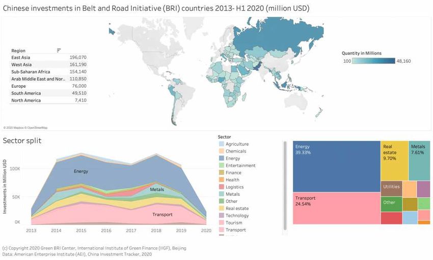
7

135 on the global warming. Therefore, the present study objectives are; to investigate the impacts of

136 energy consumption, economic growth and other developmental parameters on the emissions of

137 CO2 in BRI partner countries; and to evaluate the linkages between economic growth,

138 environmental sustainability and energy growth factors in BRI countries.

139 Figure 1: Investments of China in BRI countries from 2013-H12020 (million USD) 1

140 2. Materials and Methods

141 2.1. Data and Variables

142 This study contemplates BRI-associated nations in the terrestrial locations of Europe,

143 East Asia, Pacific, Central Asia, South Asia, Middle East and North Africa. There were 49

 1 Source: https://green-bri.org/wp-content/uploads/2020/09/Investments-in-the-Belt-and-Road-Initiative-
 BRI-2020-1024x614.png

8

144 countries selected from those regions based on the data available (Please see list of countries in

145 Table 1A).

146 The present study used CO2 as dependent variable and other variables mentioned in Table

147 1 considered independent variables. The dataset has been log-transformed for the purpose of

148 standardization. This standardization will minimize the robustness from data and will minimize

149 the enlargement of coefficients, multi-correlations and autocorrelations related problems. The

150 description and sources of all the variables have been stated in Table 1.

151 Table.1 Data Description and Symbolization

 Variables Description

 Energy consumption (EC) Litres to kilograms energy usage per capita

 Metric tones of CO2 atmospheric release per
 Carbon emission (CO2)
 capita

 Percent of GDP (total inflow of foreign direct
 Foreign Direct Investment (FDI)
 investment)

 Trade friendliness/openness (TOP) Trade (% of GDP)

 Financial development (FD) Percent of GDP (private sector domestic credit)

 Industry (medium and high-tech) (MHI) MHI as percent of value added manufacturing

 REC as percent of total final energy
 Renewable energy consumption (REC)
 consumption

 GDP per capita with a constant o 2010 US
 Gross domestic product (GDP)
 dollars

 2
152

153 2.2. Steps for Econometric analyses

 2 Source: https://data.worldbank.org/

9

154 To test the hypothesis for the underlying variables, i.e., CO2, ECON, FD, GDP, FDI,

155 MHI, TOP, and REC a primary equation is formed (Equation-1). Based on several recent studies

156 e.g. (Al-Mulali et al. 2015, Behera &Dash 2017, Doğan et al. 2021, Gulistan et al. 2020, Haseeb

157 &Azam 2020, Khan et al. 2020, Khan et al. 2019, Rauf et al. 2020, Saboori &Sulaiman 2013) the

158 following relationship among variables under investigation in this study has been developed;

159 CO2 = ( , , , FDI, , , , ) (1)

160 Here in Eq. 1, Carbon dioxide as mentioned earlier is the dependent variable and

161 relationship will be estimated as “CO2 is equal to the function of independent variables”. The

162 econometric analysis for this study comprises the following steps. (i) Analysis of the descriptive

163 statistics such as correlation analysis for the selected variables for this study. (ii) Testing the

164 dependence (cross-sectional) of the countries data to confirm that the estimate drawn from the

165 dataset is reliable. Afterwards, co-integration checkup based on the results can verify long-run

166 integrated forms amongst the variables (Al-Mulali et al. 2013). (iii) Fully Modified OLS

167 (FMOLS) and Dynamic OLS (DOLS) models for equilibrium relationships. Finally, (iv) The

168 Panel Heterogeneous Granger causality test will be used to detect interconnectivity as used by

169 Rauf et al. (2018a).

170 Equation 1 is an appropriate representation of the base model. The base model is

171 rewritten with the natural log form of data and equation 2 is formed.

172 CO2 i,t = α + β1 lnECONi,t + β2 lnFDi,t + β3 lnGDPi,t + β4 lnFDIi,t + β5 lnMHIi,t + β6 lnTOPi,t

173 + β7 lnRECi,t + εi,t (2)

10

174 Whereas, i = number of countries, t = time, ln = natural logarithm, α = intercept, β =

175 slope to the parameters, and εi,t = error terms for the equation.

176 2.2.1. Dependency test (Cross-sectional)

177 Testing cross-sectional dependency of variables is critical to form any econometric

178 model. Cross-sectional dependence (CD) is an important test in large data econometric modeling.

179 It should be checked by investigators before evaluating investigation of any group. The existence

180 or not of such a violation will correct the auxiliary path, which must be followed later. If the

181 information in the dataset has a cross-sectional dependency, the other phases of the analysis

182 should retain tests that are consistent with the cross-sectional dependency.

183 In structured variables, the cross dependence based on residuals can be examined by LM test

184 (Breusch &Pagan 1980), scaled LM test (bias-corrected) (Baltagi et al. 2012) and CD test

185 (Pesaran 2004). “No” cross-sectional dependence among that residual based dataset is the Null

186 hypothesis.

187 Therefore, both the CD and LM test are structured in the following ways:

 −1 2 2
 2 ( − ) ̂ − ( − ) ̂ 
188 = √ (∑ ∑ ̂ ) 2 (3)
 ( − 1) ( − ) ̂ 
 =1 = +1

 −1 
 2 
189 = √ (∑ ∑ ̂ ) ~ (0,1) , = 1,2,3 … 65 … (4)
 ( − 1)
 =1 = +1

11

 2
190 Whereas, ̂ is residuals correlation, which was valued by using Ordinary Least Square

191 equation. The results of the above given equations are given below in Table 2 with 1% level of

192 significance for Null hypothesis (H⁰).

193 Table.2 Results of (CD) Test

 Test Statistic

 LM of Breusch-Pagan 11392.35***

 LM of Pesaran scaled 210.6577***

 Bias-corrected scaled LM 209.6777***

 CD by using Pesaran 73.54330***

194
 1
 Note: “***” represent 1% level of significance.

195 The cross dependence of the dynamic panels for residuals of dataset has been

196 investigated by using CD tests of Frees (Frees 1995, 2004) Friedman (1937) and Pesaran (2004).

197 The short term and large cross-sectional residual dependence for given dataset (time and number

198 of countries) gave a clear understanding about the relationship between the countries over the

199 given time period. The results (Table 3) of these tests rejected Null hypothesis of cross-section

200 independence.

201 Table.3 Results of (CD) test of the residuals

 Test Statistic

 Pesaran CD test 73.54330***

 Friedman test 265.9161***

 Frees test 7.504881***

202
 1
 Note: “***” represent 1% level of significance.

12

203 2.2.2. Unit Root Tests

204 The unit root tests are of two types. First type considers the self-determining power of

205 CD of target countries. The 2nd type/generation test allows the CD of the countries. The current

206 study used both types of unit root tests to provide strong justification of stability in the results.

207 The current panel's data acknowledges that there are longer-term events, which could increase

208 the degree of independence (d.f) and exacerbate the multidimensional crisis to assess the

209 equation of OLS. Therefore, panel data can withstand more compelling scientific techniques and

210 asymptomatic statistics, which follow a general distribution rather than a noise distribution.

211 Choi(Choi 2006) deviced the panel unit root test with opposite assumption/hypothesis

212 like Hadri (2000). Levin et al. (2002) used restricting type of panel unit root test for samples of

213 the finite properties while Im et al. (2003) also advised heterogenous panel unit root test.

214 Therefore, this study applies the LLC, IPS, and ADF Fisher Chi-square test for testing the

215 unit root (Table 10) to hold the order of cointegration among the variables under this study. In

216 this connection, the panel unit root test of IPS is depicted with the following equation:

217 ∆ , = + , −1 ∑ ∆ , − + , = 1, … = 1, … (5)
 =1

218 Equation 5 above depicts , as the dataset containing countries for time but the lag

219 operators are denoted with “∆”. Here, , stands for the error term for the normally distributed

220 sample BRI countries.

221 The results (Table 2 and Table 3) show the cross dependence in the dataset. Therefore,

222 we need to apply 2nd type of CD tests to justify the hitch of cross-dependence. Pesaran(Pesaran

13

223 2007) defined the process of cross-sectional Im, Pesaran, and Shin (CIPS) and cross-sectional

224 augmented Dickey-Fuller (CADF). The country to county cross-sectional dependence, reliability

225 and steadfastness will be the outcomes of these two methods with their natural heterogeneity.

226 Therefore, the test may further be built as follows:

227 ∆ , = + , −1 + ̅ −1 + ∑ ∆ ̅ , − + ∑ ∆ ̅ , − + , = 1, … (6)
 =0 =1

228 Whereas; = constant, ̅ = mean of cross-section at “t” period, and = lag operator.

229 Supposing (N, TM) same as the time ratio of , the mean of t-ratios (time ratios) will be as

230 follows;

 ∑ 
 =1 , ( , , )
231 ( , ) = (7)
 
232 Here, , ( , , ) is Augmented Dickey-Fuller (CADF) indicators for the ℎ cross-sections.

233 2.2.3. Co-integration Tests

234 The results of both types of unit root tests approved the stability of dataset. Co-

235 integration tests by Pedroni (1999), (Pedroni 2004) can further validate the level of co-

236 integration. Robustness can be confirmed by using Wetserlund co-integration test (Westerlund

237 2007) to get dependency of cross sections. The base of co-integration test is Engle-Granger (a

238 typical unit root test) which has been further expanded by Westerlund et al. (2015). Also see (Al-

239 Mulali et al. 2012, Ciarreta &Zarraga 2010 (Khan et al. 2017, Rauf et al. 2018a) for the purpose

240 of determining long-run connectivity between candidate variables. Therefore, it has been verified

241 that all given variables together formulated into first order (Equation 1).

14

242 Likewise, The Pedroni cointegration test augmented the following equation:

243 2 , = + + 1 , + 3 , + 2 , + 4 , + 5 , +

244 + 5 , + 5 , + , (8)

245 = 1, … = 1, … 

246 Whereas, is constant for each country, and is the full panel deterministic trends of

247 the particular country. There were eleven statistical results of the Pedroni co-integration test

248 while investigating both hypotheses. is homogenous for null hypothesis and its heterogeneous

249 for alternative hypothesis. The co-integration among variables can be seen in Table 9. The

250 uniformity between the target variables has been found normally distributed, which verifies the

251 Pedroni co-integration test. This relationship could be written as following equation;

 ′ − √ 
252 √ , → (0,1) (9)
 √ 

253 In equation 9, and V stand for the Monte Carlo oriented adjustment measures.

254 The first four results of Panels (v, rho, PP, and ADF statistics) in the Table 9 are within-

255 dimension statistics and latter three Groups (rho, PP and ADF) are between the dimension

256 statistics. Therefore, we have at least 4 statistics out of 7 fulfills the lowest criterion for long-run

257 linear co-integration approval within target variables.

258 After the approval of cross dependence between the target variables, the co-integration

259 test by Westerlund (2007) has the ability to produce stable and vigorous results for the approval

260 of the co-integration level. The results of (Westerlund 2007) are present in the form of two

261 groups/forms. The first group is called cluster based group (Gt and Ga), whereas, other group is

15

262 called panel statistics group (Pt and pa) (Rauf et al. 2018a, Saud et al. 2019) as shown in Table 8.

263 The results show that co-integration exists among CO2 and all other independent variables for all

264 the 49 countries of the study regions.

265 2.2.4. The Dynamic Panel Data Estimation

266 The FMOLS valuation proposed by Pedroni(Pedroni 2001) and the DOLS valuation

267 proposed by (Kao &Chiang 2001) and (Stock &Watson 1993) that have been used in this recent

268 study to explore the long-run co-integration amongst variables.

269 Meanwhile, the following FMOLS and DOLS equations are presented to test the hypotheses:

 N T
 ∑ (x −x̅ )(y −y
 ∑ ̅ )−Tγ
 ̂i
270 β̂NT = [ i=1 t=1∑T it(x i−x̂ it)2 i ] (10)
 t=1 it i

 ̂ 21i
 Ω
271 Where γ̂i = Γ̂21i + Ω
 ̂ 021i − (Γ̂ ̂ 222i )
 +Ω
 Ω21i 22i
 ̂

272 And ̂i = Ω
 Ω ̂ 0i + Γ̂i + Γ̂′i

273 ̂ = long-run matrix of stationarity, Ω
 Whereas, Ω ̂ 021 = term to reject the covariance b/w

274 errors terms of stationarity, and Γ̂ = modified covariance between independent variables.

275 2.2.5. Heterogeneous Panel Causality test

276 At the last stage of econometric analysis, the panel Granger causality test has been used

277 to find the instrumental correlation between target variables under investigation in the study.

278 3. Results and Discussions

16

 279 The present study used a series of correlational and cross-sectional dependence tests to

 280 develop understanding about the effects of energy growth, financial development, GDP, medium

 281 and high-tech industries, trade openness and renewable energy consumption on the emissions of

 282 Carbon Dioxide (CO2). The results presented in the form of series of Tables to clearly represent

 283 the outcomes of the present study for the regions and countries of the study. The empirical

 284 results obtained through current investigation can help the policy makers to achieve “Green BRI”

 285 goals in regional panels.

 286 3.1. Descriptive Statistics

 287 The summary of statistics has been presented in Table 4 comprising 49 countries and

 288 1274 observations dataset. The variables data has been standardized by using natural logarithm

 289 to avoid heteroscedasticity. The consumption of energy was a trending variable with the mean of

 290 1945.1240 and a standard deviation of 2698.9130. The mean emissions of CO2 were lower

 291 (5.0492) in million tons but it was highly variable in the different countries of the different

 292 regions. This type of variation indicates the different level of advancement in individual

 293 countries. Similarly, mean GDP of the overall countries in the panel was higher (2698.9130)

 294 with lower standard deviation indicating the improved state of economy of the countries of the

 295 regions under investigation. The mean value of FD and MHI had similar outcomes (38.2041 and

 296 24.4740 respectively) indicating their strong dependence on each other. Similarly, TOP and FDI

 297 shows similar trends in the given time span.

 298 Table 4. Descriptive Statistics

Variable→ CO2 EC FD FDI GDP MHI REC TOP

Mean 5.0492 1945.1240 38.2041 4.0261 2698.9130 24.4740 17.6670 88.0877

17

Median 2.9844 899.8239 33.4432 2.7452 4456.3600 24.0068 6.0378 81.1580

Maximum 35.9158 12406.7500 165.3904 54.2391 64864.7200 88.0370 92.3802 437.3267

Minimum 0.0000 0.0000 0.0000 -40.4143 0.0000 0.0000 0.0000 0.0000

Std. Dev. 6.4352 2698.9130 34.1423 5.5015 11334.0600 17.0908 23.1835 58.3168

Skewness 2.1786 2.2411 1.0170 2.3774 2.4375 0.6725 1.4498 2.0877

Kurtosis 7.9716 7.7552 3.8979 26.4151 9.4368 3.6670 4.2063 11.1954

Jarque-Bera 2319.8320 2266.6950 262.4066 30303.8600 3460.9280 119.6407 523.5765 4490.7950

Probability 0.0000 0.0000 0.0000 0.0000 0.0000 0.0000 0.0000 0.0000

Sum 6432.74 2478088 48672.04 5129.211 11037057 31179.84 22507.74 112223.7

Observations 1274 1274 1274 1274 1274 1274 1274 1274

 299

 300 3.2. Correlation Analyses

 301 The present study correlation analyses results show the highly significant positive

 302 correlation between CO2 and GDP (0.7153 ***) MHI (0.2564***), EC (0.8063***), FD

 303 (0.08291***) and TOP (0.2080***) respectively. There was highly significant negative

 304 correlation found between CO2 and REC (-0.3956***) and as shown in Table 5. There was no

 305 significant correlation found between CO2 and financial development (FDI). The results of

 306 strong association between GDP, MHI, and EC and CO2 has also been observed by Rauf et al.

 307 (2020). But current study result contradicts the weak correlation results of CO2 and FD with

 308 (Rauf et al. 2020). Therefore, it can be easily observed that CO2 emissions are mainly connected

 309 with the GDP of the countries, medium and high-tech industries, and energy consumption as

 310 correlation statistics indicated clearly about it. These indicators are main drivers of the

 311 atmospheric CO2 emissions and controls the atmospheric conditions through increased

 312 greenhouse gas emissions in the countries under current investigation. Therefore, the two-way

18

313 correlation estimated provides a good insight into series of datasets. However, it is important to

314 further validate the results and develop cross sectional relationships to cross validate the

315 established preposition.

316 Table 5. Correlation Statistics

 Variab TOP
 le CO2 EC FD FDI GDP MHI REC

 CO2 1.0000

 EC 0.8063** 1.0000
 *

 FD 0.08291* 0.0577** 1.0000
 **

 FDI 0.02907 0.0815** 0.1795** 1.0000
 * *

 GDP 0.7153** 0.5745** 0.2331** 0.1343** 1.0000
 * * * *

 MHI 0.2564** 0.2280** 0.3897** 0.0835** 0.4267** 1.0000
 * * *

 REC - - - - - - 1.0000
 0.3956** 0.3394** 0.2230** 0.1180** 0.3904** 0.2234**
 * * * * * *

 TOP 0.2080** 0.2283** 0.3752** 0.4265** 0.4050 0.4427** - 1.000
 * * * *** * 0.2271** 0
 *
 1
317 *, **, *** shows statistical significance at the 10%, 5% and 1% respectively.

318 3.2.1. Unit Root tests and Slope Homogeinity

319 This study used first-generation/type LLC, IPS and ADF (Table 6) and second-

320 generation/type CIPS and CADF (Table 7) of unit root tests for data stationarity checking. The

321 stationarity of individual variables examined and results indicated the difference between

19

322 variables in panels of study regions. Some of the unit roots tests discarded the null hypothesis at

323 their level, the stationarity at 1st order has been supported by most of the tests. The results of CD

324 test showed strong cross dependence between variables. Further, study examined the slope

325 heterogeneity test for heterogenous panels in Table 8. The Pedroni and Kao based tests (1st type

326 /generation co-integration tests) might face the issue of lower co-integration between the

327 variables. To avoid this problem with Pedroni and Kao based co-integration tests, the

328 (Westerlund 2007) has been used to estimate the level of co-integration between study variables,

329 (see (Yasmeen et al. 2018). The Pedroni co-integration test gave strong evidence of rejecting null

330 hypothesis through 4 out of 7 values having higher significance level “p”. The results of

331 Westerlund co-integration test under the cross-dependence situation proved to be the best choice

332 as shown in Table 9 which validates the long-run co-integration between variables. The results of

333 Pedroni (Table 10) and Kao (Table 11) shows the high level of co-integration among all

334 variables in long-run. Further investigations using FMOLS and DOLS models will give insight

335 into the long-run co-integration in full and regional panels.

336 Table 6. Panel Unit Root test results (LLC, IPS and ADF)

 At level

 Methods CO2 EC FD FDI GDP MHI REC TOP

 - -
 Levin, Lin & 6.2575 9.0830 0.3153 7.1973 2.7861 31.398 4.9201 20.249
 Chu t* 8 5 7 5*** 7 2 6 6***

 - -
 Im, Pesaran 6.1258 7.9944 1.9067 8.4359 5.7933 5.9824 6.2350 13.017
 and Shin 3 0 7 6*** 8 4 7 0***

 ADF - Fisher 45.207 13.920 75.935 256.12 65.704 48.270 51.045 174.24
 Chi-square 5 1 2 5*** 6 1 6 9***

20

 At first Difference

 Methods CO2 EC FD FDI GDP MHI REC TOP

 - - - - - - -
 Levin, Lin & 16.771 18.418 4.3673 16.701 301.09 186.93 28.892 117.81
 Chu t* 6*** 0*** 5*** 8*** 0*** 6 3*** 7***

 - - - - - - -
 Im, Pesaran 14.256 13.997 12.679 21.985 80.347 0.8861 24.521 54.980
 and Shin 9*** 8*** 0*** 1*** 1*** 1 3*** 0***

 ADF - Fisher 383.61 374.26 362.66 614.25 395.85 136.90 651.30 751.82
 Chi-square 9*** 5*** 6*** 8*** 7*** 9*** 0*** 1***
 1
337 *, **, *** shows statistical significance at the 10%, 5% and 1% respectively.

338 Table 7. Results of CIPS and CADF (Panel unit root tests)

 At Level

 Metho CO2 EC FD FDI GDP MHI REC TOP
 ds

 - - -
 - 6.093** 3.825** 3.049** -
 CIPS 2.679** * -2.169 * * -2.202 2.696** -2.401

 - -
 3.033** 3.131** -
 CADF -2.256 -1.633 * * 2.539** -2.179 -1.929 -1.923

 1st Deference

 Metho CO2 EC FD FDI GDP MHI REC TOP
 ds

 - - - - - - - -
 2.679** 6.320** 4.939** 5.793** 4.616** 4.459** 4.732** 4.419**
 CIPS * * * * * * * *

 - - - - - - - -
 3.896** 3.638** 3.491** 4.580** 3.411** 3.352** 3.168** 3.373**
 CADF * * * * * * * *
 1
339 *, **, *** shows statistical significance at the 10%, 5% and 1% respectively.

21

340 Table 8. Testing for slope heterogeneity

 Delta P-value

 17.394*** 0.000

 Adj. 21.512*** 0.000
 1
341 *, **, *** shows statistical significance at the 10%, 5% and 1% respectively.

342 Table 9. Westerlund test of Cointegration

 Statistic Value Z-value P-value

 Gt -13.126*** -49.216 0.0000

 Ga -19.064* 11.516 0.058

 Pt -56.338*** -4.123 0.0000

 Pa -24.097*** 8.456 0.0000
 1
343 *, **, *** shows statistical significance at the 10%, 5% and 1% respectively.

344 Table 10. Pedroni test of Cointegration

 Weighted

 Panel and Group statistics Statistic Probability Statistic Probability.

 v-Statistic (Panel) 2.5574*** 0.0053 -0.0548 0.5219

 rho-Statistic (Panel) 1.8471 0.9676 1.2252 0.8898

 PP-Statistic (Panel) -2.7401*** 0.0031 -5.6625*** 0.0000

 ADF-Statistic (Panel) -7.7309*** 0.0000 -8.2642*** 0.0000

 rho-Statistic (Group) 4.2118*** 1.0000

 PP-Statistic (Group) -5.3655*** 0.0000

 ADF-Statistic (Group) -7.7040*** 0.0000
 1
345 *** shows statistical significance at 1% significance level.

22

346 The Kao co-integration test employed to validate the results of Pedroni co-integration tests. The

347 result of Kao test showed -13.18381*** (Table 11), which clearly indicates that the previously

348 applied integration tests were efficient and Kao test results are authenticating those previously

349 obtained outcomes of co-integration. The similar results found in the study by (Rauf et al. 2018b)

350 where their results of Pedroni co-integration tests were validated by Kao co-integration test.

351 Table 11. Kao test of Cointegration

 t-Statistic Prob.

 ADF -13.18381*** 0.0000

 Residual variance 0.126030

 HAC variance 0.111819
 1
352 *** shows statistical significance at 1% significance level.

353 3.2.2. Dynamic Panel data models

354 The estimations obtained from co-integration test validated the long term relationship among

355 variables which gave strong reason to apply FMOLS and DOLS to get stable outcomes(Pedroni

356 2001); (Pedroni 2004). Both DOLS and FMOLS has been used to establish the expected

357 relationship between the regressor and the regressed. The results shown in Table 12 clearly

358 reveals that EC, FDI, GDP, and MHI found unfavorably influencing the environmental quality

359 through carbon dioxide emissions. These results can be validated by results obtained from (Rauf

360 et al. 2020). Renewable energy consumption (REC), and trade openness (TOP) have favorable

361 effect on the environment. (Rauf et al. 2018b) also found that trade openness do not have

362 negative effects on the environment in BRI partner countries.

23

363 Table 12. Results for FMOLS and DOLS for countries undder investigation

 Regressor: CO2 Emissions

 Panel-49 BRI countries

 Variables Coefficients

 FMOLS DOLS

 LNEC 0.173604*** 0.282734***

 LNFD 0.000992 0.031297

 LNFDI 0.044221** 0.054350

 LNGDP 0.438718*** 0.467377***

 LNMHI 0.170090*** -0.155954

 LNREC -0.306305*** -0.482432***

 LNTOP -0.002527 0.015257

 R-squared 0.869660 0.999602

 Adjusted R-squared 0.862954 0.989165
 1
364 *, **, *** shows statistical significance at the 10%, 5% and 1% respectively.

365 Precisely, it can be observed from the results of FMOLS that 1% increase in energy

366 consumption EC, FDI, GDP and MHI leads to the degradation of environment (CO2 emissions)

367 having strong relationship of 0.173604***, 0.044221**,0.438718***,and

368 0.170090***respectively. The results of both models (DOLS and FMOLS) found to have been

369 similar in terms of developing relationship between regressor and the regressed ones. We can

370 summarize from the results of both models that the 49 countries studied need to understand that

371 economic growth, medium and high-tech industries and foreign direct investments should

372 transform their sources of energy generation from fossil fuel based to renewable energy

373 generation sources. These findings reveal that level of emissions of CO2 in the BRI partner

24

374 countries is dependent on the consumption of energy. The increased magnitude of the energy

375 consumption will cause the increased impact on the environment. It further leads the researchers

376 to emphasis mainly on the innovation-based advancements. The adaptation of energy efficient

377 technologies can reduce the burden on energy generation sector (Choi et al. 2012), which will

378 ultimately have reduced impact on the ecological health of the countries. Therefore, it is strongly

379 recommended to promote renewable energy generation and sharing of environment friendly

380 technologies among the BRI partner countries for sustainable economic growth with minimum

381 impact on the ecological health of the partner countries. In this regard, the Green BRI initiative is

382 the good step to promote the environment friendly technologies and options for sustainable

383 energy, economy and environmental growth in BRI partner countries. The current study results

384 infers similar outcomes to (Apergis &Ozturk 2015, Arouri et al. 2012, Atici 2009, Bekhet

385 &Othman 2017, Hafeez et al. 2018, Jalil &Mahmud 2009, Khan et al. 2017, Nasir &Rehman

386 2011, Omri 2013, Rauf et al. 2018b, Xu &Lin 2016b). The option of carbon free technologies

387 such as nuclear, biomass based, wind turbines, hydropower, and solar energy and their associated

388 technologies can transform the growth patterns of BRI partner countries with improved

389 environmental quality. (Javid &Sharif 2016) found similar findings for Pakistan, (Zhang &Gao

390 2016) and (Xu &Lin 2016b) for China, (Kasman &Duman 2015) for European Union members,

391 ((Rauf et al. 2018a); (Rauf et al. 2020); (Rauf et al. 2018b) for BRI member countries.

392 3.2.3. The Panel granger causality analysis

393 The causality between CO2 and independent variables has been investigated using Granger panel

394 causality analysis. (Dumitrescu &Hurlin 2012) developed the causality test, which also addresses

395 the problem of heterogeneity among variables. Therefore, the causality test by (Dumitrescu

396 &Hurlin 2012) has been used in the present study for the selected BRI countries. The divergent

25

397 results of causality test found for the 49 BRI partner countries in the present study. The results of

398 Granger causality test are presented in Table 12. The results are showing quite clear causal

399 relationship of CO2 with other variables. Energy consumption has unidirectional (one way)

400 relationship with CO2 emissions, while financial development, GDP, MHI and REC showed

401 bidirectional (feedback type) relationship with CO2. Foreign direct investment (FDI), and TOP

402 has inverse unidirectional relationship with CO2. The resultant pathways of relationship of

403 independent variable with environmental health will help the policymakers to let them develop

404 sustainable and environment friendly strategies in BRI partner countries.

405 Table 13. Dumitrescu Hurlin Panel Causality analysis

 Null Hypothesis: Zbar-Stat. Prob. Relationship directions

 LNEC ≠ LNCO2 46.9575*** 0.0000
 LNEC → LNCO2
 LNCO2 ≠ LNEC 0.56576 0.5716

 LNFD ≠ LNCO2 40.5894*** 0.0000
 LNFD ↔ LNCO2
 LNCO2 ≠ LNFD 21.5626*** 0.0000

 LNFDI ≠ LNCO2 -0.44992 0.6528
 LNFDI ← LNCO2
 LNCO2 ≠ LNFDI 4.27438*** 0.0000

 LNGDP ≠ LNCO2 2.21961** 0.0264
 LNGDP ↔ LNCO2
 LNCO2 ≠ LNGDP 8.40507*** 0.0000

 LNMHI ≠ LNCO2 -2.6427*** 0.0082
 LNMHI ↔ LNCO2
 LNCO2 ≠ LNMHI 181.943*** 0.0000

 LNTOP ≠ LNCO2 1.28659 0.1982
 LNTOPG ← LNCO2
 LNCO2 ≠ LNTOP 23.939*** 0.0000

 LNREC ≠ LNCO2 80.8119*** 0.0000
 LNREC ↔ LNCO2
 LNCO2 ≠ LNREC 2.2346** 0.0254

406

26

407 This causal relationship between target variables clearly justifies the high rate of CO2

408 emissions connectedness with the economic advancement (Table 13). It conclusively defines the

409 influence of economic growth on the environmental health in the BRI partner countries. Carrying

410 on these kind of economic development activities may lead to the increased global warming

411 along with unprecedented type of human health effects. The possible solution of such negative

412 thrust back of economic growth is the adaption of technologically advanced and green solutions.

413 These type of causal relationships are also found in studies by (Al-Mulali et al. 2015, Katircioglu

414 2017); (Rauf et al. 2020, Saud et al. 2019)).

415 3.3. Checking regression robustness

416 The results of DOLS and FMOLS presented to see robustness (Table 11), this study

417 applies the Dynamic Seemingly Unrelated Regression (DSUR). The purpose of applying DSUR

418 is to check the robustness in the oucomes obtained from FMOLS and DOLS tests. The results

419 presented in Table 14 shows that there was medium to high impact of indicators under

420 investigation on emissions of Carbon dioxide (R2 = 0.60) in the countries under investigation in

421 the present study.

422 Table 14. Dynamic seemingly unrelated regression results

 Panel Variable Coefficient z-Statistic Prob.

 LNEC 0.1559787*** 24.67 0.0000

 LNFD -0.0285969** -2.51 0.0120

 LNFDI 0.0584332*** 3.96 0.0000

 LNGDP 0.3897101*** 21.37 0.0000

 49 BRI countries LNMHI 0.1741924*** 9.93 0.0000

27

 LNREC -0.243571*** -21.03 0.0000

 LNTOP 0.0600654*** 3.76 0.0000

 CONSTANT -3.481891*** -23.78 0.0000

 R-squared 0.7559

 Chi Square 3944.86***

423

424 The results of DSUR endorse the results obtained by using FMOLS and DOLS, where

425 EC, FDI, GDP and MHI are major drivers of the environmental degradation (Table 14). Trade

426 openness and renewable energy consumption favored the environment as also found in FMOLS

427 and DOLS test results. The indicator of FD has not been found with significant relationship with

428 the emissions of CO2, having similar results as previously used both models.

429 4. Conclusions

430 The present study conducted to examine the impacts of energy consumption, GDP,

431 financial development, renewable energy consumption, foreign direct investment, and medium

432 and high-tech industry on the emissions of Carbon dioxide (CO2) in 49 nations on the panel of

433 Belt and Road initiative. The duration of investigation expands from 1994 to 2019. The robust

434 type of panel cross-section dependence and slope heterogeneity and other methods were adopted

435 to analyze the dataset of BRI countries under investigation. The standardized (log-transformed)

436 data has been used to employ slope heterogeneity, cross-sectional dependency of the panel data

437 to confirm that the estimate drawn from the dataset is reliable.

438 Afterwards, panel tests (co-integration tests) used to verify the long-term integrated forms

439 amongst the variables and, FMOLS and DOLS models used for long-term equilibrium

440 relationship among the variables. Finally, The Panel Heterogeneous Granger causality test

28

441 applied to detect the interconnectivity between variables at causal bases (mainly CO2 emissions

442 with other independent variables). The consumption of energy (EC) along with foreign direct

443 investment (FDI), medium and high-tech industry (MHI) and GDP has been found highly

444 unfavorable for the ecological health (CO2 emissions) in 49 nations on BRI panel. However,

445 renewable energy consumption (REC) has been found a favorable impact on the environment

446 quality parameter (CO2). There was no significant impact of financial development (FD)

447 indicator on CO2 emissions has been observed in the present study.

448 More precisely, the energy consumption, medium and high-tech industries and GDP has

449 been the major variables found in all analytical outcomes, those having highly significant

450 impacts on the environmental quality/health (CO2 emissions). However, the adaptation of

451 renewable energy sources has been found in significantly obliging impacts (favorable) in all

452 analytical outcomes with ecological health of the countries in BRI panel. The present outcomes

453 clearly claim the strong relationship of economic growth with increased CO2 emissions in all 49

454 nations under investigation of Belt and Road initiative.

455 Therefore, it can be concluded that the huge investments of Chinese government under

456 BRI projects on energy sector (mainly based on fossil fuel-based energy generation) along with

457 industrial sector development are driving factors behind the environmental deterioration in those

458 countries. However, the impacts of BRI projects on environment can be minimized using

459 renewable energy generation sources especially those of carbon free energy generation

460 technologies. Further, the industrial pollution can also be minimized through regulating them

461 according to the environmental standards. The governments of BRI listed countries can

462 formulate sustainable options of green energy, green transport, green innovation and green

463 standards, which are in line with the initiative taken by Ministry of Ecology and Environment of

29

464 China. Present study can provide a strong justification of sustainable economic growth for the

465 policy makers of BRI partner countries while keeping in mind the environmental implications.

466 The transfer of technology between the partner countries can also help to transform the economic

467 growth into an energy efficient and sustainable development.

468 The estimates of recent study suggest some essential policy implications for lawmakers

469 and environmental experts. They must allocate economic resources based on the results of the

470 study to maximize productivity, but wisely. As a result, researchers will take short- and long-

471 term approaches to environmental issues, in particular the involvement of greenhouse gases

472 (GHGs) and the BRI economy’s climate change sensitivity. This shows that continued economic

473 expansion is the key to improving the quality of the environment. Thus, for all regions tested to

474 reduce CO2 emissions, more practical and stringent policies / strategies are needed from decision

475 makers and stakeholders. In addition, the various estimates of the current study are a useful tool

476 for developing renewable energy supply strategies to avoid the risk of (GHG) emissions not only

477 for the BRI partnered nations but it will be great gadget for larger countries of the world. It is

478 also important to anticipate demand and supply of energy to achieve the development of BRI

479 projects. In addition, improved GDP per capita (income) will allow the general public with the

480 provision of more dynamic and environment friendly services. Therefore, it is also important for

481 policy makers to incentivize and appreciate investors for green investment and inform them

482 about its benefits.

483 Additionally, researchers can modify variables that may produce points that can further

484 help to improve the understanding about the impacts of BRI projects investments on

485 Environment in general and on the regional climate in particular. In addition, we could measure

486 the relationship of energy and economic growth indicators with many other climate change and

30

487 environment related indicators, like natural disasters, global warming, oxides of nitrogen, oxides

488 of sulfur, Carbon Monoxide, industrial pollution and health effects, in order to obtain an overall

489 environmental impression.

490 Appendix A

491 Table A1: List of Selected BRI countries

 S.No Countries S.No Countries

 1 Albania 26 North Macedonia

 2 Armenia 27 Mongolia

 3 Azerbaijan 28 Moldova

 4 Bahrain 29 Maldives

 5 Bangladesh 30 Malaysia

 6 Belarus 31 Myanmar

 7 Bosnia and Herzegovina 32 Nepal

 8 Bulgaria 33 Oman

 9 Cambodia 34 Pakistan

 10 Colombia 35 Philippines

 11 Croatia 36 Romania

 12 China 37 Russian Federation

 13 Czech Republic 38 Poland

 14 Egypt, Arab Rep. 39 Saudi Arabia

 15 Georgia 40 Singapore

 16 Hungary 41 Slovak Republic

 17 India 42 Sri Lanka

 18 Indonesia 43 Thailand

31

 19 Iran, Islamic Rep. 44 Turkey

 20 Israel 45 Tajikistan

 21 Jordan 46 Ukraine

 22 Kazakhstan 47 Yemen, Rep.

 23 Kyrgyz Republic 48 United Arab Emirates

 24 Kuwait 49 Vietnam

 25 Lebanon

492

493

494

495

496

497

498

499

500

501

502

503

504

32

505 References

506 Al-Mulali U, Sab CNBC, Fereidouni HG (2012): Exploring the bi-directional long run
507 relationship between urbanization, energy consumption, and carbon dioxide emission.
508 Energy 46, 156-167
509 Al-Mulali U, Fereidouni HG, Lee JY, Sab CNBC (2013): Exploring the relationship between
510 urbanization, energy consumption, and CO2 emission in MENA countries. Renewable
511 and Sustainable Energy Reviews 23, 107-112
512 Al-Mulali U, Tang CF, Ozturk I (2015): Does financial development reduce environmental
513 degradation? Evidence from a panel study of 129 countries. Environmental Science and
514 Pollution Research 22, 14891-14900
515 Apergis N, Ozturk I (2015): Testing environmental Kuznets curve hypothesis in Asian countries.
516 Ecological Indicators 52, 16-22
517 Arouri MEH, Youssef AB, M'henni H, Rault C (2012): Energy consumption, economic growth
518 and CO2 emissions in Middle East and North African countries. Energy policy 45, 342-
519 349
520 Atici C (2009): Carbon emissions in Central and Eastern Europe: environmental Kuznets curve
521 and implications for sustainable development. Sustainable Development 17, 155-160
522 Ayeche MB, Barhoumi M, Hammas M (2016): Causal linkage between economic growth,
523 financial development, trade openness and CO2 emissions in European Countries.
524 American Journal of Environmental Engineering 6, 110-122
525 Balsalobre-Lorente D, Shahbaz M, Roubaud D, Farhani S (2018): How economic growth,
526 renewable electricity and natural resources contribute to CO2 emissions? Energy Policy
527 113, 356-367
528 Baltagi BH, Feng Q, Kao C (2012): A Lagrange Multiplier test for cross-sectional dependence in
529 a fixed effects panel data model. Journal of Econometrics 170, 164-177
530 Behera SR, Dash DP (2017): The effect of urbanization, energy consumption, and foreign direct
531 investment on the carbon dioxide emission in the SSEA (South and Southeast Asian)
532 region. Renewable and Sustainable Energy Reviews 70, 96-106
533 Bekhet HA, Othman NS (2017): Impact of urbanization growth on Malaysia CO2 emissions:
534 Evidence from the dynamic relationship. Journal of cleaner production 154, 374-388
535 Breusch TS, Pagan AR (1980): The Lagrange multiplier test and its applications to model
536 specification in econometrics. The review of economic studies 47, 239-253
537 Cai X, Che X, Zhu B, Zhao J, Xie R (2018): Will developing countries become pollution havens
538 for developed countries? An empirical investigation in the Belt and Road. Journal of
539 Cleaner Production 198, 624-632
540 Chen H (2016): China’s ‘One Belt, One Road’initiative and its implications for Sino-African
541 investment relations. Transnational Corporations Review 8, 178-182
542 Choi I (2006): Combination unit root tests for cross-sectionally correlated panels. Econometric
543 Theory and Practice: Frontiers of Analysis and Applied Research: Essays in Honor of
544 Peter CB Phillips. Cambridge University Press, Chapt 11, 311-333
545 Choi Y, Zhang N, Zhou P (2012): Efficiency and abatement costs of energy-related CO2
546 emissions in China: A slacks-based efficiency measure. Applied Energy 98, 198-208
547 Ciarreta A, Zarraga A (2010): Economic growth-electricity consumption causality in 12
548 European countries: A dynamic panel data approach. Energy policy 38, 3790-3796

33

549 Doğan B, Driha OM, Balsalobre Lorente D, Shahzad U (2021): The mitigating effects of
550 economic complexity and renewable energy on carbon emissions in developed countries.
551 Sustainable Development 29, 1-12
552 Dombrowski K (2017): Clean at Home, Dirty Abroad
553 Du J, Zhang Y (2018): Does one belt one road initiative promote Chinese overseas direct
554 investment? China Economic Review 47, 189-205
555 Dumitrescu E-I, Hurlin C (2012): Testing for Granger non-causality in heterogeneous panels.
556 Economic modelling 29, 1450-1460
557 Economy W (2017): UNDP Says BRI Can Create Sustainable Growth. Financial Tribune
558 Fan J-L, Zhang Y-J, Wang B (2017): The impact of urbanization on residential energy
559 consumption in China: An aggregated and disaggregated analysis. Renewable and
560 Sustainable Energy Reviews 75, 220-233
561 Finance IIfG (2021): Green Belt and Road initiative center, Central University of Finance and
562 Economics
563 Frees EW (1995): Assessing cross-sectional correlation in panel data. Journal of econometrics
564 69, 393-414
565 Frees EW (2004): Longitudinal and panel data: analysis and applications in the social sciences.
566 Cambridge University Press
567 Friedman M (1937): The use of ranks to avoid the assumption of normality implicit in the
568 analysis of variance. Journal of the american statistical association 32, 675-701
569 Grossman GM, Krueger AB (1995): Economic growth and the environment. The quarterly
570 journal of economics 110, 353-377
571 Gulistan A, Tariq YB, Bashir MF (2020): Dynamic relationship among economic growth,
572 energy, trade openness, tourism, and environmental degradation: fresh global evidence.
573 Environmental Science and Pollution Research 27, 13477-13487
574 Hadri K (2000): Testing for stationarity in heterogeneous panel data. The Econometrics Journal
575 3, 148-161
576 Hafeez M, Chunhui Y, Strohmaier D, Ahmed M, Jie L (2018): Does finance affect
577 environmental degradation: evidence from One Belt and One Road Initiative region?
578 Environmental Science and Pollution Research 25, 9579-9592
579 Haseeb M, Azam M (2020): Dynamic nexus among tourism, corruption, democracy and
580 environmental degradation: a panel data investigation. Environment, Development and
581 Sustainability, 1-19
582 Ho D (2017): Cost of funding ‘Belt and Road Initiative’is daunting task. South China Morning
583 Post 27
584 Im KS, Pesaran MH, Shin Y (2003): Testing for unit roots in heterogeneous panels. Journal of
585 econometrics 115, 53-74
586 Intelligence FB (2017): Available online: (accessed on 03 January, 2021)
587 http://www.iberchina.org/files/2017/OBOR_Business_Implications_Fung.pdf
588 IPCC 2014: Intergovernmental Panel on Climate Change Fifth Assessment Report
589 Jalil A, Mahmud SF (2009): Environment Kuznets curve for CO2 emissions: a cointegration
590 analysis for China. Energy policy 37, 5167-5172
591 Jaunky VC (2011): The CO2 emissions-income nexus: evidence from rich countries. Energy
592 Policy 39, 1228-1240
593 Javid M, Sharif F (2016): Environmental Kuznets curve and financial development in Pakistan.
594 Renewable and Sustainable Energy Reviews 54, 406-414

34

595 Kao C, Chiang M-H (2001): On the estimation and inference of a cointegrated regression in
596 panel data, Nonstationary panels, panel cointegration, and dynamic panels. Emerald
597 Group Publishing Limited
598 Kasman A, Duman YS (2015): CO2 emissions, economic growth, energy consumption, trade
599 and urbanization in new EU member and candidate countries: a panel data analysis.
600 Economic modelling 44, 97-103
601 Katircioglu S (2017): Investigating the role of oil prices in the conventional EKC model:
602 evidence from Turkey. Asian Economic and Financial Review 7, 498-508
603 Khan MK, Teng J-Z, Khan MI (2019): Effect of energy consumption and economic growth on
604 carbon dioxide emissions in Pakistan with dynamic ARDL simulations approach.
605 Environmental Science and Pollution Research 26, 23480-23490
606 Khan MK, Khan MI, Rehan M (2020): The relationship between energy consumption, economic
607 growth and carbon dioxide emissions in Pakistan. Financial Innovation 6, 1-13
608 Khan MTI, Yaseen MR, Ali Q (2017): Dynamic relationship between financial development,
609 energy consumption, trade and greenhouse gas: comparison of upper middle income
610 countries from Asia, Europe, Africa and America. Journal of cleaner production 161,
611 567-580
612 Kuznets S (1955): Economic growth and income inequality. The American economic review 45,
613 1-28
614 Levin A, Lin C-F, Chu C-SJ (2002): Unit root tests in panel data: asymptotic and finite-sample
615 properties. Journal of econometrics 108, 1-24
616 Liu Y, Hao Y (2018): The dynamic links between CO2 emissions, energy consumption and
617 economic development in the countries along “the Belt and Road”. Science of the total
618 Environment 645, 674-683
619 Musolesi A, Mazzanti M, Zoboli R (2010): A panel data heterogeneous Bayesian estimation of
620 environmental Kuznets curves for CO2 emissions. Applied Economics 42, 2275-2287
621 Nasir M, Rehman FU (2011): Environmental Kuznets curve for carbon emissions in Pakistan: an
622 empirical investigation. Energy policy 39, 1857-1864
623 Omri A (2013): CO2 emissions, energy consumption and economic growth nexus in MENA
624 countries: Evidence from simultaneous equations models. Energy economics 40, 657-664
625 Pedroni P (1999): Critical values for cointegration tests in heterogeneous panels with multiple
626 regressors. Oxford Bulletin of Economics and statistics 61, 653-670
627 Pedroni P (2001): Fully modified OLS for heterogeneous cointegrated panels, Nonstationary
628 panels, panel cointegration, and dynamic panels. Emerald Group Publishing Limited
629 Pedroni P (2004): Panel cointegration: asymptotic and finite sample properties of pooled time
630 series tests with an application to the PPP hypothesis. Econometric theory, 597-625
631 Pesaran MH (2004): General diagnostic tests for cross-sectional dependence in panels. Empirical
632 Economics, 1-38
633 Pesaran MH (2007): A simple panel unit root test in the presence of cross‐section dependence.
634 Journal of applied econometrics 22, 265-312
635 Petroleum B (2017): BP statistical review of world energy 2017. Br. Pet 66, 1-52
636 Rauf A, Liu X, Amin W, Ozturk I, Rehman OU, Hafeez M (2018a): Testing EKC hypothesis
637 with energy and sustainable development challenges: a fresh evidence from belt and road
638 initiative economies. Environmental Science and Pollution Research 25, 32066-32080