What Drives Social Returns to Education? A Meta-Analysis - DISCUSSION PAPER SERIES
←
→
Page content transcription
If your browser does not render page correctly, please read the page content below
DISCUSSION PAPER SERIES

IZA DP No. 14332

What Drives Social Returns to Education?
A Meta-Analysis

Ying Cui
Pedro S. Martins

APRIL 2021
DISCUSSION PAPER SERIES

IZA DP No. 14332

What Drives Social Returns to Education?
A Meta-Analysis

Ying Cui
Queen Mary University of London
Pedro S. Martins
Queen Mary University of London and IZA

APRIL 2021

Any opinions expressed in this paper are those of the author(s) and not those of IZA. Research published in this series may
include views on policy, but IZA takes no institutional policy positions. The IZA research network is committed to the IZA
Guiding Principles of Research Integrity.
The IZA Institute of Labor Economics is an independent economic research institute that conducts research in labor economics
and offers evidence-based policy advice on labor market issues. Supported by the Deutsche Post Foundation, IZA runs the
world’s largest network of economists, whose research aims to provide answers to the global labor market challenges of our
time. Our key objective is to build bridges between academic research, policymakers and society.
IZA Discussion Papers often represent preliminary work and are circulated to encourage discussion. Citation of such a paper
should account for its provisional character. A revised version may be available directly from the author.

                                           IZA – Institute of Labor Economics
Schaumburg-Lippe-Straße 5–9                      Phone: +49-228-3894-0
53113 Bonn, Germany                             Email: publications@iza.org                                    www.iza.org
IZA DP No. 14332 APRIL 2021
ABSTRACT
What Drives Social Returns to Education?
A Meta-Analysis*
Education can generate important externalities that contribute towards economic growth
and convergence. In this paper, we study such externalities and their drivers by conducting
the first meta-analysis of the social returns to education literature. We analyse over 1,000
estimates from 32 journal articles published since 1993, covering 15 countries of different
levels of development. Our results indicate that: 1) there is publication bias (but not citation
bias) in the literature; 2) spillovers slow down with economic development; 3) tertiary
schooling and schooling dispersion increase spillovers; and 4) spillovers are smaller under
fixed-effects and IV estimators but larger when measured at the firm level.
JEL Classification: I26, I28, J24, J31, C36
Keywords: returns to education, education externalities
Corresponding author:
Pedro S. Martins
School of Business and Management
Queen Mary University of London
Mile End Road
London E1 4NS
United Kingdom
E-mail: p.martins@qmul.ac.uk
* We thank comments from Jampel Dell’Angelo, Maria Koumenta and Yong Yang. Cui thanks financial support
from the China Scholarship Council (20180806431). All errors are our own.1 Introduction
The social effects of education may go much beyond the individuals that are investing directly in
their own human capital. A person’s education, or schooling, may affect different outcomes of their
colleagues at work, neighbours, and possibly even other people in the same region, industry or even
country (Marshall 1890). To the extent that education shapes an individual’s own thinking, actions,
and outcomes - as clearly indicated by a large literature on the private returns of education -, one’s
learning at school can also influence different economic and non-economic variables regarding other
individuals. Specific economic examples include higher productivity and earnings. Non-economic
outcomes may include better informed political participation, increased tax revenues, lower required
public expenditure, lower crime, and slower spread of diseases (perhaps also during pandemics), all of
which can again also lead to higher productivity and earnings.
Given their significance and breadth, such spillovers from schooling can promote economic de-
velopment and convergence. The latter will apply if education spillovers are higher when economic
development is lower. Indeed, the examples above may suggest that the marginal social return to
education is higher at lower levels of economic development. For instance, if crime or the spread of
disease tends to be higher at lower levels of economic development and if education tends to reduce
crime or the spread of disease, then the social effects of education may be greater when countries are
at earlier stages in their development. Many of these social effects would be translated into pecuniary
dimensions, including productivity and wages.
Moreover, education spillovers may follow from non-pecuniary external returns (technological
spillovers or knowledge diffusion) or, alternatively, pecuniary external returns (market interactions
and prices) (Moretti 2004, Cardoso et al. 2018). In the latter case, more schooling in the general
workforce may incentivise firms to invest in their physical and organisational capital which may make
even the less schooled more productive. However, note that schooling could theoretically also have
negative external effects, namely in the context of signaling models. Overall, the considerable poten-
tial for schooling spillovers or externalities - and the underlying inefficiency from education provided
exclusively by markets - has therefore motivated large public investments in education. For instance,
according to the World Bank, over 15% of governments’ total expenditure is devoted to education,
corresponding to an average of 4% of GDP.
In this paper, we seek to better understand social returns to education and its drivers, including
the role of economic development. Our contribution is to conduct what we believe is the first meta-
analysis of the microeconomic literature that estimates these external effects of education.1 According
1
For a meta-analysis of the related but different macroeconomic literature, on the relationship between education and
2to our review, that we describe in more detail below, there are 32 journal articles in the literature that
researches the magnitude of different types of education spillovers. These studies cover 15 countries
(and four continents), of which five address the cases of emerging or developing economies (China,
Indonesia, Kenya, South Africa, and Tunisia), representing in total 33.1% of the world population.
To be able to better compare the studies, we focus on the studies that estimate pecuniary outcomes
at the microeconomic level. We then analyse the extent to which the literature suffers from publication
and citation biases. The former concerns the more likely publication of particular results, namely those
with positive effects. The second type of bias, which we borrow from the medical literature, concerns
the extent to which particular results, namely positive effect, are more likely to be cited by other
papers. Moreover, we also study the role of a number of contextual and methodological variables.
We find some evidence of publication bias (but not of citation bias). Our results are also supportive
of the hypothesis above, namely that spillovers slow down with economic development. Moreover, we
also find that tertiary schooling and schooling dispersion increase spillovers; spillovers are smaller
under fixed-effects and IV estimators but larger when measured at the firm level. These results can be
helpful in allowing researchers to better compare their findings with other studies that adopt different
methodological approaches.
The remaining of the paper is organised as follows. Our data are described in Section 2. The
research design and results are presented in Section 3. This includes both the analysis of publication
and citation biases as the analysis of the drivers of the social and external returns along multiple
dimensions of each study. The final section concludes.
2 Data and variables
2.1 Criteria for selecting studies
Our selection of studies was based on a comprehensive Google Scholar search (see Sokolova & Sorensen
(2021) for a recent meta-analysis using a similar approach). More specifically, we included the following
keywords in our search: ’education externalities’, ’human capital externalities’, ’education spillovers’,
’social returns to education’ and ’external returns to education’ (using the ’OR’ operator). These
keywords capture the different phrases that authors have used to refer to the concept of externalities
in education. Our search was originally conducted in May 2020 and considered the first 30 pages of
results delivered by Google Scholar (each page listing ten different papers).
Following the initial stage above, we then considered the studies that met the following subject and
economic growth, see Benos & Zotou (2014). See also Glewwe et al. (2014).
3methodological criteria. On the subject side, we considered only studies that focused on at least one of
three key economic outcomes we are interested in here: productivity (of firms), wages, and rents (land).
These have been identified before as three main avenues for education spillovers (Moretti 2004): more
educated workers can drive upwards the productivity of the firms in which they are employed, which
can then increase the wages of all employees (through some combination of rent/profit sharing and
labour market competition); finally, increases in productivity and wages in locations where schooling
spillovers are large can lead to increases in rental prices.
On the methodological side, our inclusion criteria were the following. First, we consider exclusively
studies published in academic journals listed in ABS (2018). This widely used journal ranking list
includes over 300 journals in economics alone; however, it also includes over 1,000 additional journals
from other disciplines and subjects taught at business schools, including those which may also study
the social effects of education from a quantitative perspective.2 Second, we include exclusively those
estimates that are reported in the main text of the paper (excluding estimates in appendices, many of
which based on subsamples or different sets of control varriables). We also required that the number
of observations, the time period considered in the estimation (and other variables discussed below)
are clearly reported.3 Finally, we also conducted a complementary search based on EconLit, following
the same criteria as above. This delivered 87 studies in a first instance. However, we added only
one journal article, published in 2019, to our original selection as the remaining studies either did not
meet our criteria described above or were already included in our sample following the Google Scholar
analysis.
In summary, we collected a total of 1,021 estimates from 32 empirical studies on education
spillovers. The full list of articles can be found in Appendix A. While the number of papers is
relatively small compared to more mature literatures that have already been subject to meta-analysis,
the number of estimates in our study is relatively large (e.g. larger than in Benos & Zotou (2014)).
Morever, our estimates cover as many as 15 countries (and four continents), namely China, Denmark,
Germany, Hungary, Indonesia, Italy, Kenya, Netherlands, Portugal, Russia, South Africa, Switzerland,
Tunisia, UK, and US.4 These 15 countries represent 33.1% of the world population and provide a good
coverage of different levels of schooling and economic development.
2
These subjects include human resource management, industrial relations, international development, and operations
research. Considering this broader list can make our study selection more inclusive, leading to a broader range of
approaches and a larger number of studies and estimates. In any case, we also consider an alternative journal list,
focused on economics, as we explain below.
3
We also considered Acemoglu & Angrist (2000) and Rudd (2000), which were not published in journals but are
widely cited in the literature. On the other hand, we excluded one very short study which reported only three estimates.
4
This analysis also indicates that some the most important gaps in the geographical coverage of existing published
studies in education externalities are in India and Latin America. Eastern Europe and East Asia (e.g. Japan, South
Korea) have also not been considered in the literature. These gaps may affect the generalizability of our results and
constitute areas where further research may be particularly welcome.
42.2 Explanatory variables
We characterise the studies in this literature and their estimates along nine dimensions. These dimen-
sions lead to 29 variables that we then consider as potential predictors of the size of the spillover that
we analyse, following our discussion above. These dimensions and their variables are as follows:
1. Spillover measure: We consider the cases of the average years of schooling and the share of
college-educated workers. The former is more comprehensive while the latter is more focused on the
individual profiles that may have greater potential to generate spillovers, given the more advanced type
of their schooling. Of course, levels of schooling below college, such as secondary school completion,
may also be relevant, particularly in less developed countries where average education levels are lower.
Note that we do not consider studies that focus on spillovers from qualitative types of education, such
as vocational education as opposed to academic schooling, or particular courses in higher education
(e.g. engineering or humanities).
2. Spillover scope: These have been classified as regional, industry, or firm levels. These three
dimensions correspond to the levels at which the potential spillovers (such as the average years of
schooling and share of college-educated workers) may be generated and are measured in the empirical
analyses. As discussed before, schooling externalities can arise and be measured within different
dimensions, related to the location (region or country) of the individuals, the sector or industry in
which they work, or within their firm (a specific combination of sector and location in most cases,
namely in firms located in a single area). For instance, if the average years of schooling (or college-
educated share) adopted in the study are calculated within a city/region, then we define the spillover
scope of that study to be the regional level. Alternatively, if the measures are calculated within each
firm (industry), by considering the relevant schooling measure of those workers, we then define the
scope as the firm (industry) level. A common specification involves regressing the log of a worker’s
wage on a number of human capital (control) variables, plus a measure of the average schooling of the
individuals in the same firm, region or industry.5
3. Spillover outcome: The effects of spillovers may arise in multiple variables. In this meta-
analysis, we consider the cases of the productivity of firms, the wages of workers, and rental prices. As
discussed above, spillovers are likely to arise in terms of productivity in a first instance, as co-workers
(in the same firm, industry and or region) benefit from the skills of more educated individuals. This
will increase the productivity of those co-workers and their firms. Such productivity increases will
then lead to wage increases through some combination of market competition for more productive
5
For instance, Martins & Jin (2010) conducts the analysis at the firm level, constructing the key regressor as the
average schooling of all, same-firm colleagues of each worker. The wages of the latter are then considered as the dependent
variable.
5workers and rent sharing from firms to their workers. Higher regional wages and profits driven by the
spillovers can also translate into higher prices for those resources in limited and rigid supply, such as
land and housing, driving increases in rents. These higher rents may lead to some convergence of real
wages across locations that are endowed with workforces of different schooling (and spillover) levels.
4. Spillover type: The literature studies both the social returns to education and the external
returns to education. The latter can be regarded as the additional returns, accrued from interactions
with other schooled individuals, that can be added to the direct, private returns. When the direct
and indirect components are taken together, they would correspond to social returns. In other words,
SR = P R + ER, in which SR, PR and ER are, respectively, the social returns, the private returns
and the external returns. If the model considered in the paper under analysis considers separately
the individual’s schooling (as an additional control variable) and then focuses on ’social’ schooling,
we regard the coefficient of the later as a measure of the external return, over and above the private
return. If there is no such control for individual’s schooling (and their private returns), then the
coefficient (regarding total schooling in a given region, for instance) is regarded as a social return, as
it will capture both direct and indirect dimensions.
5. Data set characteristics: Studies draw on the main types of data sets used in (micro-)econometric
analyses, namely single cross-sections, pooled cross-sections, and panel data. The case of panel data
sets are based on repeated observations of individuals or firms over time. We also considered the time
period examined in each study as well as the size of the sample (number of observations).
6. Estimation method: Several estimates are obtained from OLS. However, many studies seek
to address the potential endogeneity of their schooling variable through fixed effects (drawing on the
repeated availability of the same individuals over time), instrumental variables or other methods. In
some studies, their estimates draw on more than one such method, namely when combining instrumen-
tal variables and fixed effects. These data points (estimates) are classified correspondingly - unlike in
the previous dimensions, the multiple potential outcomes are not mutually exclusive in this dimension
regarding the estimation method.
7. Country income level: As discussed in the Introduction, social returns to education may vary
depending on the income level of the country under analysis. We examine this by classifying the
country studied in each article in four income levels: high, upper-middle, lower-middle and low. Using
the World Bank Atlas method, these correspond to GNI per capita in 2018 of $12,376 or more, between
$3,996 and $12,375, between $1,026 and $3,995, and $1,025 or less, respectively.
8. Schooling quantity and quality: The underlying levels of schooling in each country may also
influence its social returns. We consider both quantity and quality dimensions, measured in terms
6of the percentage of university graduates and the average schooling years (quantity) of the country’s
workforce (Barro & Lee 2013) and the average PISA scores across its three dimensions (maths, science
and reading results). We use the measurement for the same year as that of the data when the social
return is estimated or the closest possible (the latter in the case of the PISA scores).
9. Publication characteristics: We are also interested in uncovering potential relationships between
the publication characteristics of each article and the social returns documented there. We consider
four different variables in this case, namely the year of publication, the number of (Google Scholar)
citations, and the journal ranks. The latter is measured using (ABS 2018), a widely used journal
ranking including over 300 journals in economics alone plus over 1,000 journals from related fields
taught at business schools (some of which may also examine social returns to education). We consider
five journal categories (from ’recognised world-wide as exemplars of excellence’, the top level (’4*’,
which we score as 5), to ’recognised, but more modest standard in their field’, the bottom level, which
we score as 1). For the benefit of further robustness, we also measure the journal rank using the article
influence score from the Eigenfactor database (link).
2.3 Descriptive statistics
The descriptive statistics of the variables described above are presented in Table 1. These statistics
are computed from the 1,021 individual estimates that we extracted from 32 empirical studies (journal
articles), treating each estimate equally, and provide an interesting overview of the literature. First,
we find that most estimates are computed at the regional level (86%), while the industry and firm
levels represent only 5% and 9% of the total, respectively. In contrast, we find considerable balance
in the measurement of the potential spillovers, as 58% of the estimates use average years of schooling
and 42% use the share of college-educated workers.
Wages prove to be the key outcome of education spillovers (82% of the estimates), followed by
(firm) productivity (15%), while rents play a residual role (only 2% of the cases). Most studies focus
on the external returns to education as they consider specifications that control for individual schooling
(64% of the observations). The remaining 36% do not control for individual schooling and are thus
interpreted here as estimating social returns to education (including both direct and indirect effects).
We find considerable dispersion in data types across our sample of studies: 25% of the estimates
come from single cross-sections, 49% from pooled cross-sections, and 26% from panel data. Similarly,
36% of the estimates use OLS only, 22% use fixed effects (involving repeated observations of the units
upon which the externalities may arise, e.g. firms or regions), 26% use instrumental variables (listed in
Table B.3), and the remaining 20% use different methods (GLS, Heckman’s selection and multilevel
7modelling). These statistics also indicate that in only 1% of the cases are there overlaps between the
different methods, which correspond to the joint use of fixed effects and instrumental variables.
When considering the economic development of the countries studied, we find that the majority
the estimates (76%) are high-income. 19% are upper-middle income and only 5% are lower-middle
income (no country covered is in the low income category). These statistics highlight the geographical
dispersion of the existing estimates, but also the relatively limited evidence available from lower-
income, developing countries. As discussed above, the latter may be the ones where social returns
to education are the highest, given their relatively lower average schooling levels and the potentially
greater impact of schooling from a social perspective.
Across the countries and time periods considered, we find an average percentage of graduates of
14% and 10.1 years of schooling. Again, these relatively large means reflect the large percentage of
estimates from developed countries and recent years, following significant expansions of the education
systems of developing countries.
Interestingly, the average number of observations used in each estimate is very large, at 288,000
(even if this is driven mostly by one particular study which studies around eight million observations).
Moreover, on average, the estimates concern data regarding the year of 1990, even if the full range of
years is very wide, starting at 1950 and ending in 2010. In contrast, the year of (journal) publication
of the articles is, on average, 2007, covering the period 1993 to 2020.
Finally, the journals where the estimates are published are typically well reputed, with an average
ABS (2018) ranking of 3.19 (and median of 3), where 5 is the maximum (namely the ’top five’ journals
in economics) and 1 the minimum (typically journals of limited international scope). Using the article
influence score measure, the mean is 2.47 (and median of 1.6). The (log) number of Google scholar
citations is 4.63 (about 100 citations), with a maximum of 7.49 (nearly 1,800, Rauch (1993)).
3 Results
3.1 Methodology
To investigate the drivers of social returns, we perform a meta-analysis by estimating the following
equation:
k
βˆij = α0 +
X
αk Xjk + eij , (1)
k=1
8where βˆij is the ith estimate from the j th study and Xjk are the meta-independent variables that
follow from the study design as described above.
However, note that in our analysis the estimated effects are not necessarily directly comparable
as they are diverse along different dimensions. For instance, we consider in this study both the social
returns to education and the external effects of education, depending on the approach adopted in each
paper. Some estimates concern years of schooling while others the share of university graduates. The
dependent variables include productivity, wages and rents. In order to analyse all estimates from the
multiple studies jointly, we transform the estimated effects into partial correlation coefficients (PCC).
The PCCs, which measure the association of a dependent variable and the independent variable, are
widely used in economic meta-analyses to standardise effect sizes.
The formula we use is:
tij
P CC(β̂ij ) = q , (2)
t2ij + dfij
where tij is the t-statistic of the effect under study and dfij are the degrees of freedom for the ith
estimation in the j th paper. Note that several selected studies do not report the number of regressors
used, which prevent us from considering the exact value of df . In these cases, we used an approximation
of the number of regressors based on our best analysis of the information available.6 Finally, the
standard errors of the PCCs, SE, are calculated as:
s
2
1 − P CCij
SE(P P Cij ) =
dfij
We present the resulting descriptive statistics of the t-statistics and PCCs in Table 2. We find that
62.8% of the estimates indicate a significantly positive effect (at the 5% level), 33.6% are insignificant,
and 3.6% are significantly negative. The mean and median t-statistics for the full sample are 3.68
and 2.47, respectively, while the PCC values have a mean and median values of 0.04 and 0.02. The
distributions of t-statistics and PCCs are presented in Figures 1 and B.1.7
PCC values by study characteristics are presented in Table B.1, including information on the
number of estimates and their range. This analysis indicates some relevant patterns including that:
(1) PCCs are higher at the firm level (0.076); (2) PCCs tend to be lower under fixed-effects (0.016) and
IV (0.034) estimators, compared to the OLS estimator (0.043); (3) PCCs are higher when measuring
social returns (0.043) than when measuring exclusively spillovers (0.040); and (4) PCCs are (much)
6
One challenge here concerns studies based on panel data sets with a large number of individuals and a small number
of time periods, which may create a significant difference between N and df.
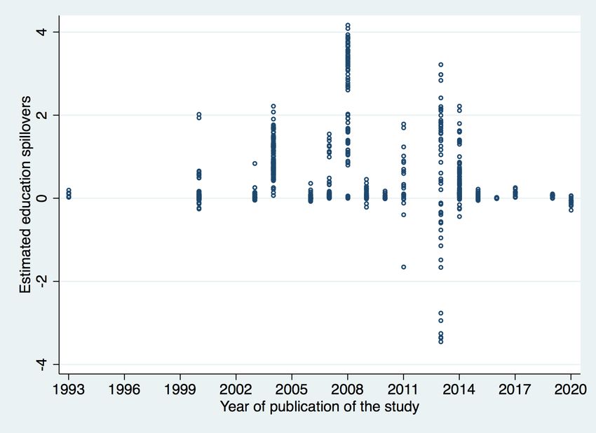
7
See also Figure B.2 which illustrates the range of estimates over the years in which they were published.
9higher in low-income economies (0.063, compared to 0.037 in high-income economies). Later in the
paper, we test the extent to which these patterns hold when considering the multiple dimensions
simultaneously under the meta-regression below.
3.2 Publication bias
An important question in the context of meta-analyses is if particular types of estimates, namely
those that are significant, are more likely to be published. Studies that find spillovers to schooling
may be regarded as more interesting and relevant in contrast to those that do not uncover significant
effects. If the former are more likely to be reported and published than the latter, such selection would
contribute to a skewed understanding of education externalities and possibly incorrect decisions from
a policy perspective.
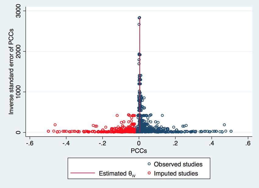
We obtain a first indication of the extent of publication bias in this literature by using the funnel
plot methodology. The funnel plot (Light & Pillemer 1984) is a scatter plot of the reported study
effect (i.e. PCCs in our case) against measures of study precision (i.e. the inverse standard errors of
PCCs). In the absence of publication bias, the shape of the scatter plot should resemble a symmetric
inverted funnel because the sampling error is random.
Figure 2 presents a funnel plot based on the data that we collected. We find that the plot is
skewed, given that the right tail is much more prominent compared to the left tail. This suggests
that a large share of negative estimates may be missing from the funnel plot, which would indicate
publication bias in the form of selection for a positive sign. However, this method of publication bias
detection is based on visual inspection only, which may lack objectivity and accuracy.
In order to provide a more rigorous analysis, next we perform a trim-and-fill analysis in order
to estimate if studies are potentially missing from our meta data set. This trim and fill method
(Duval & Tweedie 2000) involves dropping (trimming) the less precise estimates causing funnel plot
asymmetry and introducing (filling) those studies potentially missing from the meta-analysis because
of publication bias. The result of the trim and fill approach is presented in Table 4. We find that: (1)
the mean spillover effect based on the 1,021 observed estimates is 0.005; (2) there are 334 estimates
potentially missing and subsequently imputed; and (3) after including such estimates, we obtain a new
estimate (based on the observed plus imputed 1,335 estimates) of the mean spillover effect of 0.004.8
In addition to funnel plot, we also make use of the meta-regression to further detect publication
bias. We follow the FAT-PET-PEESE approach (Stanley & Doucouliagos 2012) to test whether the
8
Figure B.3 reveals that a substantial portion of negative estimates is missing from the funnel plot, due to publication
bias in the form of selection for a positive sign. As indicated before, if these missing estimates were included in the meta-
analysis, the resulting funnel plot would be more symmetrical.
10effect is genuine or influenced by publication bias. We start out by regressing the t-statistic of the k th
estimate on the inverse of the standard error (1/SE) by considering the following equation:
tk = β0 + β1 (1/SEk ) + uk . (3)
We then test the null hypothesis that the intercept term β0 is equal to zero - this corresponds
to the funnel-asymmetry test (FAT). If β0 is statistically significantly different from zero, then the
distribution of the effect sizes is regarded as asymmetric. However, regardless of publication selection,
we are also able to identify an empirical effect by testing the null hypothesis that the coefficient β1 is
equal to zero in equation 3 - this corresponds to the precision-effect test (PET). If β1 is statistically
significantly different from zero, this indicates the presence of a genuine effect.
Moreover, we can also estimate the magnitude of the empirical effect corrected for publication
selection by estimating the following equation which has no intercept:
tk = β0 SEk + β1 (1/SEk ) + uk (4)
We test the null hypothesis that the intercept term β1 is equal to zero in equation 4. If β1 is
statistically significantly different from zero, this indicates that a non-zero effect does actually exist
in the literature, and β1 can be regarded as its estimate. This corresponds to the precision-effect
estimate with standard error (PEESE) test. To test the robustness of the β coefficients in equations
3 and 4 above, we use four estimators: OLS estimator, which does not assign any weight to each
estimate; weighted least square (WLS) estimator, which uses either the inverse of the number of
estimates reported in the study as a sampling weight or the inverse of the imputed quality level of the
journal as an analytical weight; and a least square dummy variable (LSDV) estimator which controls
for study-level fixed effects. All estimation procedures calculate standard errors at the study level.
The regression results based on the FAT-PET-PEESE test for publication bias are presented in
Table 3. We find the following: First, in the FAT test, the null hypothesis that β0 = 0 of equation 3 is
rejected, which indicates the presence of publication bias. Second, in the PET test, the null hypothesis
that β0 = 0 of equation 3 is rejected as well, which implies that a true empirical effect does exist in
the literature (even if there is a publication selection bias). Finally, in the PEESE test, the coefficient
β1 in equation 4 is statistically significantly different from zero, which indicates the the magnitude of
the empirical effect corrected for publication selection is significantly positive, ranging between 0.017
and 0.02. In conclusion, we find evidence of publication bias, although the FAT-PET-PEESE test also
indicates that there is a genuinely positive spillover effect.
113.3 Citation bias
We are also interested in the novel concept of ’citation bias’, which we define as the extent to which
particular types of results tend to be cited more. Specifically, we want to know if significantly positive
estimates tend to receive more citations than other types of results. This analysis is possible given
our collection of citation counts from Google Scholar, as mentioned above.
We believe this approach is relevant as the screening or consideration of studies in the literature
can in some cases be more relevant at the citation stage than in terms of publication. Indeed, given
the large number of journals around the world, many studies are eventually published, even if only
after several rejections from journals of possibly increasingly lower average standing. In this case, the
extent to which a paper is cited may be a relevant dimension of bias in its impact on the literature.
We propose a simple method to shed light on the question above, regarding potentially higher
citations for studies of particular characteristics, namely significantly positive spillovers. Specifically,
we regress the log number of citations on the respective PCCs (its mean across estimates of each
study) in the context of the following equation:
logCj = α0 + α1 P CCij + α2 Zj + uij , (5)
where logCj is log citations of the j th study, and Zj includes two characteristics of the study
that may directly affect its citations record, namely the publication age and the imputed journal
quality. Studies published in journals of higher standing and which have been published for more
years will typically have more citations - it therefore may be useful to control for these variables.
These dimensions may or not be directly related to the magnitude of the PCC, depending on the
relevance of publication bias, which our earlier findings show to be present in this literature. We
argue that, if the coefficient α1 is statically significant and positive, that would indicate that studies
with larger spillovers are more likely to be cited. In other words, researchers would tend to pay more
attention to significant, large results, and the literature could therefore be developing a biased view
of social returns to education.
First, when we run a scatter plot of the log number of citations against the average PCC value
per study (Figure B.4), we find a negative but negligible correlation between the two variables, a
preliminary result which is not consistent with citation bias. We then present the OLS estimates
of different versions of equation 5 in Table 5. Column 1 does not include any controls, column 2
controls only for journal rank (using the more comprehensive ABS (2018) measure), column 3 controls
for both journal rank and years since publication. We find in all cases that the PCCs are not positively
12correlated with the log number of citations. This result is consistent with our preliminary evidence of
no citation bias in this literature. When considering all PCCs from the multiple estimates per study
(and clustering standard errors accordingly), we again find similar results, indicating no positive
relationship between more positive social returns and higher citation counts. Again, we find similar
results when considering our alternative measure of journal quality (Table B.2).
3.4 Drivers of social returns
We now turn to the analysis of the potential determinants of the magnitude of the social returs to
education. For the benefit of robustness, our meta-regression considers six estimators: OLS, not
assigning any weight to each estimate; meta-regression fixed-effects estimator, which weights each
estimate by the within-study variance; meta-regression random-effects estimator, which weights each
estimate by the within-study variance plus the between-studies variance; and the weighted least square
(WLS) estimator, which uses either the inverse of the number of estimates reported in the study as
a sampling weight, or the inverse of the standard error of PCCs and the imputed quality level of the
journal where the study was published as an analytical weight.9
Our main results, based on the estimation of equation 1, are presented in Table 6. These prove to
be generally very robust across all the specifications. First, we find that, compared to the regional level
(i.e. the benchmark category), spillovers are higher at the firm level, with an increase of between 0.026
and 0.065. According to our discussion above, this positive effect may arise because people engage
much more directly and intensively within firms, including through face-to-face communication. This
facilitates deeper interactions, through which the human capital obtained by each one from schooling
can more easily spillover to their coworkers. In contrast, the industry approach appears to deliver
similar results when compared to the regional level.
Second, we do not find systematic differences in the estimates of spillovers when using the share
of college-educated workers (as opposed to the average years of schooling). This result may be driven
from the fact that most variation in average years of schooling is driven by variation in college-educated
shares, at least in more developed countries (the large share of our sample).
Third, as expected, social returns are stronger than spillovers (external effects), with an increase
ranging between 0.006 and 0.068. Social returns include both the individual own effects of schooling
and the spillovers or externalities that schooling generates. To the extent that spillovers are positive,
9
Note that we do not consider the variables that are generated after the study is completed (journal rank, year
of publication, and number of citations) as potential explanatory variables of the PCC. OLS and WLS procedures
calculate standard errors clustering at the study level. We also standardized the two continuous variables, the number
of observations and time period considered, in order to make their coefficients more easily interpretable. See Martins &
Yang (2009) for another illustration of this approach in the context of a different literature.
13social returns should be greater than spillover estimates, as indeed we find in our analysis. It is
interesting that the magnitude of the coefficient is generally similar or higher than that of the intercept
of these estimates (around 0.02), which underlines the relevance of both private and extenal returns.
Fourth, compared to the benchmark OLS estimator, fixed-effects and IV estimators tend to gener-
ate weaker spillover partial correlation coefficients. This difference may be explained by upward biases
potentially present in OLS analyses. For instance, more educated workers may tend to flow to regions,
industries or firms that are more productive and that pay higher wages, regardless of the spillovers.
Such positive correlation between co-workers schooling and wages would generate a positive bias in
OLS analyses. This interpretation is consistent with the fact that IV estimators tend to lead to the
lowest PCCs of the three methods, even if not in all specifications. We present additional evidence on
this point by listing the different IVs used across studies - see Table B.3.10 On the other hand, one
can argue that it is precisely the IV estimators that deliver causal estimates of education externalities,
as they draw on explicitly exogenous variation in aggregate schooling, and therefore should receive
greater attention in this literature.
Fifth, compared to high-income economies (the benchmark category), upper-middle and lower-
middle income economies tend to exhibit larger spillover effects, ranging between 0.028 and 0.067.
Moreover, the effect from point estimates is always stronger in the case of lower-middle income
economies than upper-middle income economies. This finding may be driven by the association be-
tween income and schooling levels and the diminishing scope for spillovers as schooling levels increase,
as discussed above. If a large share of the workforce has higher levels of schooling, the scope for low-
educated workers to learn from their high-educated co-workers is weaker, leading to lower spillovers
as we find in our analysis.
Sixth, studies with more observations lead to smaller effects. Moreover, spillover effects tend
to diminish with time, although the coefficient is not always significant. The latter result may be
consistent with the finding above regarding country income levels: as a country increases its level of
development and its average education, the scope for spillovers may also be reduced. This may also
be consistent with the fact that some models indicate a downward trend over time in PCCs.
Finally, we find a potentially surprising result in that spillovers on productivity tend to be lower
than those on wages. Presumably spillovers would first arise in productivity and then part of them
would be accrued to workers in the form of higher wages. While we leave a more definite explanation for
10
From an economic perspective, a valid IV should influence the aggregate schooling variable that is driving the
spillovers without affecting directly the outcome of interest (e.g. an individual’s earnings). The table indicates that
popular IVs amongst the 18 studies listed include compulsory schooling (and child-labour) laws, lagged demographic
structures, and the presence of universities in the same region. As always, the adequacy of these and any other IVs can
be debated. Such will also depend on the context of the study, including the institutional and historical setting of the
country examined.
14this result for future research, we speculate that at least part of the answer may involve measurement
error in productivity. Measurement error is likely to be more significant in productivity than in wages,
given that wages are directly observable whereas productivity needs to be estimated, using a range of
variables that are not always present in the available data sets.
We also replicated the analysis above separately for estimates based on spillovers and social returns.
The results are presented in Tables B.4 and B.5, respectively, and are very similar to the main findings
discussed in this section.
3.5 Education levels
In an extension of our main results, we also examine the role of schooling levels in education spillovers.
As discussed before, we consider both quantity and quality measures and, with respect to the former,
both tertiary schooling and overall schooling years. We test the hypotheses that tertiary schooling
and or higher quality of schooling may generate stronger spillover effects.
Additionally, we consider the hypothesis that greater dispersion in the distribution of schooling
may increase education spillovers. In the limit, if every worker has the same level of schooling, a higher
level of schooling for the entire workforce may not generate spillovers in the sense that there are no
schooling gaps that would facilitate learning for some workers from their more-educated colleagues.
Specifically, we re-estimate our main specification from equation 1, which is now extended to
include the three new variables above: share of tertiary graduates, average schooling years, and
average schooling quality (as measured from PISA tests). Note that, when controlling for (holding
constant) average schooling, increases in the share of tertiary graduates must imply a relative increase
in low-educated workers and a relative decrease in medium-educated workers and consequently an
increase in the dispersion of schooling.11
Table 7 presents the results of this new specification. First, we find that the coefficients of the
remaining variables than schooling levels remain unchanged from our main results, at least qualitatively
when not also quantitatively. Second, the new results indicate that tertiary schooling has a statistically
significant positive effect on education spillovers, while average schooling has a statistically significant
negative effect. Finally, we do not find significant relationships between PISA scores and education
spillovers.
As discussed above, we interpret the opposite signs of the coefficients of the two education quantity
variables as supporting the relevance of dispersion in schooling as a driver of education spillovers. In
11
Note that, in the new specification, we drop a number of less developed countries as we have no information on
schooling quality there. We thus also drop the economic development measures that we used before, given the significant
multicollinearity between the two.
15this respect, increases in tertiary education may be a particularly relevant source of such externalities.
This result is in line with our finding from the previous subsection regarding the role of economic
development in that it is associated with large increases in tertiary education.
Our finding about the lack of a statistically significant positive association between schooling
quality and education spillovers is potentially related to the same mechanism regarding education
dispersion described above. Higher levels of schooling quality - as measured by PISA - may be
particularly relevant for workers with compulsory schooling (when the PISA measurement takes place).
This may boost their labour market perspectives but also reduces the potential learning from more
schooled colleagues, thus diminishing the resulting spillovers. Any statistical noise in the PISA scores
regarding schooling quality will also attenuate the effects that can be measured in our approach.
4 Conclusions
Education can generate important externalities and motivate the considerable involvement of gov-
ernments in this sector around the world. Such externalities may also be stronger at lower levels of
education. In this paper, we study the drivers of education externalities by conducting the first meta-
analysis of the social returns to education literature. We analyse over 1,000 estimates from 32 journal
articles published between 1993 and 2020, covering 15 countries in total, of which five are emerging
or developing economies.
In a nutshell, our results indicate that: 1) there is evidence of publication bias but not of citation
bias; 2) spillovers fall with economic development; 3) spillovers tend to be smaller under fixed-effects
and IV estimators but larger when measured at the firm level; and 4) tertiary schooling and schooling
dispersion tends to increase spillovers.
Overall, we believe our results highlight the relevance of the literature on social returns to education
and the importance of its findings for national and international policy as well. In particular, these
findings support the continuing investment in schooling - including tertiary education - in developing
countries as they highlight the stronger social role of education at lower levels of economic development.
Education may promote world development both from an individual private perspective and through
the higher social returns that it generates across poorer countries. From an academic perspective, our
results allow researchers to better compare their findings with respect to the existing literature, in
particular studies developed under different methodologies.
16References
ABS (2018), Academic journal guide, Report, Chartered Association of Business Schools, London.
Acemoglu, D. & Angrist, J. (2000), ‘How large are human-capital externalities? Evidence from com-
pulsory schooling laws’, NBER Macroeconomics Annual 15, 9–59.
Barro, R. J. & Lee, J. W. (2013), ‘A new data set of educational attainment in the world, 1950–2010’,
Journal of Development Economics 104, 184–198.
Benos, N. & Zotou, S. (2014), ‘Education and economic growth: A meta-regression analysis’, World
Development 64, 669–689.
Cardoso, A. R., Guimaraes, P., Portugal, P. & Reis, H. (2018), The Returns to Schooling Unveiled,
IZA Discussion Paper 11419, Institute of Labor Economics.
Duval, S. & Tweedie, R. (2000), ‘Trim and fill: a simple funnel-plot–based method of testing and
adjusting for publication bias in meta-analysis’, Biometrics 56(2), 455–463.
Glewwe, P., Maga, E. & Zheng, H. (2014), ‘The Contribution of Education to Economic Growth: A
Review of the Evidence, with Special Attention and an Application to Sub-Saharan Africa’, World
Development 59, 379–393.
Light, R. J. & Pillemer, D. B. (1984), Summing up: the science of reviewing research, Harvard Uni-
versity Press, Cambridge, MA.
Marshall, A. (1890), Principles of economics, Macmillan, London: Macmillan.
Martins, P. S. & Jin, J. (2010), ‘Firm-level social returns to education’, Journal of Population Eco-
nomics 23(2), 539–558.
Martins, P. S. & Yang, Y. (2009), ‘The impact of exporting on firm productivity: a meta-analysis of
the learning-by-exporting hypothesis’, Review of World Economics 145(3), 431–445.
Moretti, E. (2004), Human capital externalities in cities, in ‘Handbook of Regional and Urban Eco-
nomics’, Vol. 4, Elsevier, pp. 2243–2291.
Rauch, J. E. (1993), ‘Productivity gains from geographic concentration of human capital: evidence
from the cities’, Journal of Urban Economics 34, 380–400.
Rudd, J. B. (2000), Empirical evidence on human capital spillovers, Finance and Economics Discussion
Series 2000-46, Board of Governors of the Federal Reserve System (U.S.).
17Sokolova, A. & Sorensen, T. (2021), ‘Monopsony in Labor Markets: A Meta-Analysis’, Industrial and
Labor Relations Review 74(1), 27–55.
Stanley, T. D. & Doucouliagos, H. (2012), Meta-regression analysis in economics and business, Vol. 5,
Routledge.
18Figure 1: Distribution of t-statistics
Note: Each observation corresponds to a t-statistic from an estimate. The total number of
observations is 1,021. The full list of journal articles is presented in Appendix A.
Figure 2: Funnel-Asymmetry Plot
Note: This figure plots the values of PCCs that we obtained against their inverse standard errors.
The total number of observations is 1,021.
19Table 1: Definitions and summary statistics of explanatory
variables
Variable Description Mean SD Min Max
Spillover scope
Regional level# =1, if spillovers considered at regional level 0.86
Industry level =1, if spillovers considered at industry level 0.05
Firm level =1, if spillovers considered at firm level 0.09
Spillover measure
Average years of schooling# =1, if agg schooling measured by avg schooling years 0.58
Share of college-educated workers =1, if agg schooling measured by college-educated share 0.42
Spillover outcome
Wages# =1, if estimate based on wages 0.82
Rental prices =1, if estimate based on rents 0.02
Productivity (firms) =1, if estimate based on productivity 0.15
Spillover type
Social returns to education =1, if no control for individual schooling 0.36
External returns to education# =1, if control for individual schooling 0.64
20
Data set type
Cross-section =1, if cross-section data 0.25
Pooled cross-sections# =1, if pooled cross-sections 0.49
Panel data =1, if panel data 0.26
Estimation method
OLS# =1, if OLS 0.36
FE =1, if fixed effects 0.22
IV =1, if instrumental variables 0.26
Other methods =1, if different from above 0.20
Country type
High-income # =1, if high-income country 0.76
Upper-middle income =1, if upper-middle-income country 0.19
Lower-middle income =1, if lower-middle-income country 0.05
Schooling quantity and quality
Tertiary education completed % of tertiary education graduates 0.14 0.08 0.01 0.31
Avg. years of total schooling Average years of total schooling 10.10 2.35 4.54 13.42
Continued on next pageTable 1 – continued from previous page
Variable Description Mean SD Min Max
Avg. PISA score Avg PISA maths, science and reading scores 493.47 26.60 373 528
Other data characteristics
Sample size No. of observations (in thousands) 288.60 799.62 0.05 8034.75
Time period considered Avg year of time period considered 1990.75 10.42 1950 2010
Year of publication Year of journal publication 2007.27 5.59 1993 2020
Journal rank From 1 (min) to 5 (max) (ABS 2018) 3.19 1.09 1 5
Article influence score 2.47 2.36 0.3 8.5
Log citations Log Google Scholar citations (May 2020) 4.63 1.79 0 7.49
Notes: When the grouped variables include all possible categories, the benchmark categories omitted in the subsequent analysis are indicated by #.
Low-income economies are defined as those with a GNI per capita, calculated using the World Bank Atlas method, of $1,025 or less in 2018; lower
middle-income economies are those with a GNI per capita between $1,026 and $3,995; upper middle-income economies are those with a GNI per capita
between $3,996 and $12,375; high-income economies are those with a GNI per capita of $12,376 or more. The data on ’Tertiary education completed’
and ’Avg. years of total schooling’ is from Barro & Lee (2013). The number of observations of Avg. PISA score is 851. The number of observations
of Article influence score is 750. The number of observations of Log citations is 1,008. Two studies are not ranked using (ABS 2018). The Median
21
(ABS 2018) ranking score is 3. The Median Article influence score is 1.6. The data on ’Avg. PISA score’ is from the OECD database (unavailable
for South Africa and Kenya). Also, we excluded the PISA score for China, which is only available from 2009 (and refers to a specific region of the
country), while the period in the two Chinese studies considered in the meta-analysis is 1995-1998. The total number of observations is 1,021.Table 2: Descriptive statistics for effect size variables
t-statistics PCCs
Mean 3.68 0.04
Median 2.47 0.02
Maximum 89.00 0.51
Minimum -6.00 -0.22
Std.Dev. 5.53 0.08
5% -1.13 -0.04
10% -0.22 -0.00
90% 9.09 0.12
95% 12.16 0.21
Observations 1,017 1,017
Note: When calculating the PCC, we assume that the degrees of freedom are equal to the number
of observations when the studies do not report degrees of freedom nor the number of regressors
used.
22Table 3: Testing for publication bias
FAT-PET test: t = β0 + β1 (1/SE) + u
(1) (2) (3) (4)
(OLS) (WLS) (WLS) (LSDV)
Intercept(FAT:H0 :β0 =0) 2.645 2.933 2.674 2.920
(0.424) ∗∗∗ (0.473) ∗∗∗ (0.474)∗∗∗ (0.022)∗∗∗
1/SE(PET:H0 :β1 =0) 0.014 0.014 0.014 0.017
(0.005)∗∗ (0.006)∗∗ (0.005)∗∗ (0.005)∗∗∗
Observations 1015 1015 1015 1015
R-squared 0.186 0.179 0.169 0.414
PEESE test: t = β0 SE + β1 (1/SE) + u
(1) (2) (3) (4)
(OLS) (WLS) (WLS) (LSDV)
SE 1.858 1.696 2.134 -0.396
(0.573)∗∗∗ (0.473)∗∗∗ (0.766)∗∗∗ (1.263)
1/SE(H0 :β1 =0) 0.019 0.020 0.020 0.017
(0.006)∗∗∗ (0.006)∗∗∗ (0.007)∗∗∗ (0.005)∗∗∗
N 1015 1015 1015 1015
R2 0.323 0.325 0.304 0.577
Note: OLS denotes ordinary least square,which does not assign any weight to each estimate. WLS
denotes weighted least square, which uses either the inverse of the number of estimates reported
in the study as a sampling weight (column 2), or the inverse of the quality level of the study as
an analytical weight (column 3). LSDV denotes least square dummy variables, which controls for
study-level fixed effects. All estimation procedures calculate standard errors at the study level.
The significance levels are ∗ p < 0.10, ∗∗ p < 0.05, and ∗∗∗ p < 0.01.
Table 4: Trim-and-fill analysis of publication bias
Estimates No. of estimates Effect size [95% Conf.Interval]
Observed 1021 0.005 [0.005, 0.005]
Observed+imputed 1355 0.004 [0.004, 0.004]
Note: The analysis used PCCs as effect sizes based on common-effect model. ’Imputed’ denotes
potential estimates which are missed because of publication bias.
23You can also read