AWGAN: Empowering High-Dimensional Discriminator Output for Generative Adversarial Networks
←
→
Page content transcription
If your browser does not render page correctly, please read the page content below
AWGAN: Empowering High-Dimensional Discriminator Output for Generative
                                                                  Adversarial Networks
                                                                              Mengyu Dai,* 1 Haibin Hang,* 2 Anuj Srivastava3
                                                                                                             1
                                                                                                      Microsoft
                                                                                                  2
                                                                                                University of Delaware
                                                                                 3
                                                                                   Florida State University, Department of Statistics
                                                                             mendai@microsoft.com, haibin@udel.edu, anuj@stat.fsu.edu
arXiv:2109.03378v1 [stat.ML] 8 Sep 2021

                                                                     Abstract                                    use dimension of critic output n = 1, empirical evidence can
                                                                                                                 be found that using multiple dimension n could be advanta-
                                            Empirically multidimensional discriminator (critic) output           geous. For examples, in (Li et al. 2017) authors pick differ-
                                            can be advantageous, while a solid explanation for it has
                                            not been discussed. In this paper, (i) we rigorously prove
                                                                                                                 ent ns (16, 64, 128) for different datasets; In Sphere GAN
                                            that high-dimensional critic output has advantage on distin-         (Park and Kwon 2019) their ablation study shows the best
                                            guishing real and fake distributions; (ii) we also introduce         performance with n = 1024. However, the reason for this
                                            an square-root velocity transformation (SRVT) block which            phenomenon has not been well explored yet.
                                            further magnifies this advantage. The proof is based on our             One of the contribution of this paper is to rigorously
                                            proposed maximal p-centrality discrepancy which is bounded           prove that high-dimensional critic output is advantageous
                                            above by p-Wasserstein distance and perfectly fits the Wasser-       in the revised WGAN framework. Particularly, we pro-
                                            stein GAN framework with high-dimensional critic output n.
                                                                                                                 pose a new metric on the space of probability distribu-
                                            We have also showed when n = 1, the proposed discrepancy
                                            is equivalent to 1-Wasserstein distance. The SRVT block is           tions, called maximal p-centrality discrepancy. This metric
                                            applied to break the symmetric structure of high-dimensional         is closely related with p-Wasserstein distance (Theorem 3.8)
                                            critic output and improve the generalization capability of the       and can serve as a replacement of the objective function
                                            discriminator network. In terms of implementation, the pro-          in WGAN framework especially when the discriminator
                                            posed framework does not require additional hyper-parameter          has high-dimensional output. In this revised WGAN frame-
                                            tuning, which largely facilitates its usage. Experiments on          work we are able to prove that using high-dimensional critic
                                            image generation tasks show performance improvement on               output makes discriminator more sensitive on distinguish-
                                            benchmark datasets.                                                  ing real and fake distributions (Proposition 3.10). In clas-
                                                                                                                 sical WGAN with only one critic output, the discriminator
                                                               1    Introduction                                 push-forwards (or project) real and fake distributions to 1-
                                                                                                                 dimensional space, and then look at their maximal mean dis-
                                          Generative Adversarial Networks (GAN) have led to                      crepancy. This 1-dimensional push-forward may hide signif-
                                          numerous success stories in various tasks in recent                    icant differences of distributions in the shadow. Even though
                                          years (Niemeyer and Geiger 2021; Chan et al. 2021; Han,                ideally there exists a “perfect” push-forward which reveals
                                          Chen, and Liu 2021; Karras et al. 2020; Nauata et al. 2020;            any tiny differences, practically the discriminator has dif-
                                          Heim 2019; Zhan, Zhu, and Lu 2019). The goal in a GAN                  ficulties to reach that global optimal push-forward. How-
                                          framework is to learn a distribution (and generate fake data)          ever, using p-centrality allows to push-forward distributions
                                          that is as close to real data distribution as possible. This is        to higher dimensional space. Since even an average high-
                                          achieved by playing a two-player game, in which a gener-               dimensional push-forward may reveal more differences than
                                          ator and a discriminator compete with each other and try               a good 1-dimensional push-forward, this reduces the burden
                                          to reach a Nash equilibrium (Goodfellow et al. 2014). Ar-              on discriminator.
                                          jovsky et al. (Arjovsky and Bottou 2017; Arjovsky, Chin-                  Another novelty of our framework is to break the sym-
                                          tala, and Bottou 2017) pointed out the shortcomings of us-             metry structure of the discriminator network by composit-
                                          ing Jensen-Shannon Divergence in formulating the objec-                ing with an asymmetrical square-root velocity transforma-
                                          tive function, and proposed using the 1-Wasserstein distance           tion (SRVT). In the general architecture of GAN, people
                                          instead. Numerous promising frameworks (Li et al. 2017;                assume that the output layer of discriminator is fully con-
                                          Mroueh, Sercu, and Goel 2017; Mroueh and Sercu 2017;                   nected. This setup puts all output neurons in equal and sym-
                                          Mroueh et al. 2017; Wu et al. 2019; Deshpande et al. 2019;             metric positions. As a result, any permutation of the high-
                                          Ansari, Scarlett, and Soh 2020) based on other discrepancies           dimensional output vector will leave the value of objec-
                                          were developed afterwards. Although some of these works                tive function unchanged. This permutation symmetry im-
                                              * These authors contributed equally.                               plies that the weights connected to output layer are some-
                                          Copyright © 2022, Association for the Advancement of Artificial        how correlated and this would undermine the generaliza-
                                          Intelligence (www.aaai.org). All rights reserved.                      tion power of the discriminator network (Liang et al. 2019;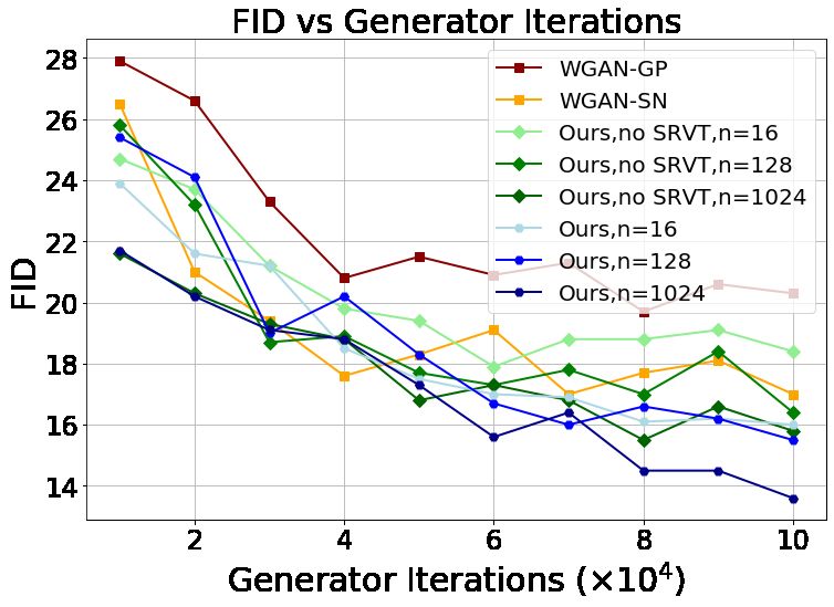
Badrinarayanan, Mishra, and Cipolla 2015). After adding            (MMD) in GAN objective, which aims to match infinite or-
the asymmetrical SRVT block, each output neuron would              der of moments. In our work we propose to use the maxi-
be structurally unique (Proposition 3.13). Our intuition is        mum discrepancy between p-centrality functions to measure
that the structural uniqueness of output neurons would im-         the distance of two distributions. The p-centrality function
ply their functionality uniqueness. This way, different output     (Definition 3.1) is exactly the p-th root of the p-th moment
neurons are forced to reflect distinct features of input distri-   of a distribution. Hence, the maximal p-centrality discrep-
bution. Hence SRVT serves as an magnifier which takes full         ancy distance we propose can be viewed as an attempt to
use of high-dimensional critic output. Since the proposed          match the p-th moment for any given p ≥ 1.
framework utilizes an Asymmetric transformation SRVT in            p-Centrality Functions: The mean or expectation of a dis-
a general WGAN framework, we name it as AWGAN.                     tribution is a basic statistic. Particularly, in Euclidean spaces,
   In terms of implementation, our experiments show perfor-        it is well known that the mean realizes the unique mini-
mance improvement on unconditional and conditional im-             mizer of the so-called Fréchet function of order 2 (cf. (Grove
age generation tasks. The novelty of our work is summarised        and Karcher 1973; Bhattacharya and Patrangenaru 2003; Ar-
as follows:                                                        naudon, Barbaresco, and Yang 2013)). Generally speaking,
1. We propose a metric between probability distributions           a Fréchet function of order p summarizes the p-th moment of
which is bounded by scaled p-Wasserstein distance. We have         a distribution with respect to any base point. A topological
theoretically proved it as a valid metric and use it in GAN        study of Fréchet functions is carried out in (Hang, Mémoli,
objectives;                                                        and Mio 2019) which shows that by taking p-th root of a
2. We utilize an asymmetrical (square-root velocity) trans-        Fréchet function, the p-centrality function can derive topo-
formation which breaks the symmetric structure of the dis-         logical summaries of a distribution which is robust with re-
criminator network. We have conducted experiments to               spect to p-Wasserstein distance. In our work, we propose
show its effectiveness in our work;                                using p-centrality functions to build a nice discrepancy dis-
3. The proposed framework improves stability of training in        tance between distributions, which would benefit from its
the setting of high-dimensional critic output without intro-       close connection with p-Wasserstein distance.
ducing additional hyper tuning parameters.                         Asymmetrical Networks: Symmetries occur frequently in
                                                                   deep neural networks. By symmetry we refer to certain
                                                                   group actions on the weight parameter space which keep
                    2    Related work                              the objective function invariant. These symmetries would
Wasserstein Distance and Other Discrepancies Used in               cause redundancy in the weight space and affects the gen-
GAN: Arjovsky et al. (Arjovsky, Chintala, and Bottou 2017)         eralization capacity of network (Liang et al. 2019; Badri-
applied Kantorovich-Rubinstein duality for 1-Wasserstein           narayanan, Mishra, and Cipolla 2015). There are two types
distance as loss function in GAN objective. WGAN makes             of symmetry: (i) permutation invariant; (ii) rescaling invari-
great progress toward stable training compared with previ-         ant. A straight forward way to break symmetry is by ran-
ous GANs, and marks the start of using Wasserstein distance        dom initialization (cf. (Glorot and Bengio 2010; He et al.
in GAN. However, sometimes it still may converge to sub-           2015)). Another way to break symmetry is via skip connec-
optimal optima or fail to converge due to the raw realization      tions to add extra connections between nodes in different
of Lipschitz condition by weight clipping. To resolve these        layers (He et al. 2016a,b; Huang et al. 2017). In our work,
issues, researchers proposed sophisticated ways(Gulrajani          we attempt to break the permutation symmetry of the output
et al. 2017; Wei et al. 2018; Miyato et al. 2018) to en-           layer in the discriminator using a nonparametric asymmet-
force Lipschitz condition for stable training. Recently, peo-      rical transformation specified by square-root velocity func-
ple come up with another way to involve Wasserstein dis-           tion (SRVF) (Srivastava et al. 2011; Srivastava and Klassen
tance in GAN (Wu et al. 2019; Kolouri et al. 2019; Desh-           2016). The simple transformation that converts functions
pande, Zhang, and Schwing 2018; Lee et al. 2019). They use         into their SRVFs changes Fisher-Rao metric into the L2
the Sliced Wasserstein Distance (Rabin et al. 2011; Kolouri,       norm, enabling efficient analysis of high-dimensional data.
Zou, and Rohde 2016) to estimate the Wasserstein distance          Since the discretised formulation of SRVF is equivalent with
from samples based on a summation over the projections             an non-fully connected network (as depicted in Fig. 2), our
along random directions. Either of these methods rely on           approach can be viewed as breaking symmetry by deleting
pushforwards of real and fake distributions through Lips-          specific connections from the network.
chitz functions or projections on to 1-dimensional space.
In our work, we attempt to distinguish two distributions by                       3    Proposed Framework
looking at their pushforwards in high dimensional space.           In this section we introduce the proposed GAN framework
This would add a lot of flexibility to convergence path which      in which the objective function is built on the maximal p-
may prevents the minimizer getting stuck on poor local op-         centrality discrepancy and the discriminator is composited
timum.                                                             with an SRVT block.
   Another way people used to distinguish real data and
fake data distributions in generative network is by moment         3.1    Objective Function
matching (Li, Swersky, and Zemel 2015; Dziugaite, Roy,             The objective function of the proposed GAN is as follows:
and Ghahramani 2015). Particularly, in (Li et al. 2017)                                      1/p                    1/p
the authors used the kernel maximum mean discrepancy                min max Ex [kD(x)kp ]         − Ez [kD(G(z))kp ]      (1)
                                                                      G    D
Proof. For any x ∈ M , by Lemma 3.2 and triangle inequal-
ity we have
|σP,p (x) − σQ,p (x)| ≤ Wp (P, Q) ≤ |σP,p (x) + σQ,p (x)|.
The result follows by letting x run over all M .
Let P(M ) be the set of all probability measures on M and
let C0 (M ) be the set of all continuous functions on M . We
define an operator Σp : P(M ) → C0 (M ) s.t. Σp (P) = σP,p .
Figure 1: The discriminator design of our framework. D0 The above lemma implies that Σp is 1-Lipschitz, which
represents a general discriminator network with multidimen- makes Σp a powerful indicator of a probability measure.
sional output. The output of its last dense layer is then trans- Specifically, since p-Wasserstein distance Wp metrizes weak
formed by the SRVT block. The p-block implements the pro- convergence when (M, d) is compact, we have:
posed objective function.
Proposition 3.4. If (M, d) is compact and P weakly con-
verges to Q, then σP,p converges to σQ,p with respect to L∞
where k · k denotes L2 norm. G and D denotes generator distance.
and discriminator respectively. p refers to the order of mo- Recall that in WGAN, the discriminator is viewed as a K-
ments. x ∼ Pr is the input real sample and z ∼ p(z) is a Lipschitz function. In our understanding, this requirement is
noise vector for the generated sample. The output of the last enforced to prevent the discriminator from distorting input
dense layer of discriminator is an n-dimensional vector in distributions too much. More precisely, in the more general
the Euclidean space Rn . setting, the following is true:
The forward pass pipeline of our framework is shown in Proposition 3.5. Given any K-Lipschitz map f :
Fig. 1. In contrast to traditional WGAN with 1-dimensional (M, dM ) → (N, dN ) and Borel probability distribu-
discriminator output, our framework allows the last dense tions P, Q ∈ P(M ). Then the pushforward distributions
layer of discriminator to have multi-dimensional output, f∗ P, f∗ Q ∈ P(N ) satisfy
which is required for further implementation of an asym-
metrical transformation (SRVT) block. We will discuss the Wp (f∗ P, f∗ Q) ≤ K · Wp (P, Q).
motivation for this transformation in Section 3.3. Here we Proof. Let Γ(P, Q) be the set of all joint probability mea-
use residual blocks as feature extractors for illustration and sures of P and Q. For any γ ∈ Γ(P, Q), we have f∗ γ ∈
implementation, while in practice they can be replaced by Γ(f∗ P, f∗ Q). By definition of the p-Wasserstein distance,
any other reasonable feature extractors.
Wp (f∗ P, f∗ Q)
3.2 The maximal p-centrality discrepancy Z 1/p
The p-centrality function was introduced in (Hang, Mémoli, = 0 inf dpN (y1 , y2 )dγ 0 (y1 , y2 )
γ ∈Γ(f∗ P,f∗ Q) N ×N
and Mio 2019) which offers a way to obtain robust topolog- Z 1/p
ical summaries of a probability distribution. In this section,
≤ inf dpN (y1 , y2 )d(f∗ γ)(y1 , y2 )
we introduce a metric on the space of probability distribu- γ∈Γ(P,Q) N ×N
tions formed by the p-centrality functions and show its re- Z 1/p
lation with the p-Wasserstein distance and an L∞ type dis- = inf dpN (f (x1 ), f (x2 ))dγ(x1 , x2 )
tance. γ∈Γ(P,Q) M ×M
Definition 3.1 (p-centrality function). Given a Borel prob- Z 1/p
ability measure P on a metric space (M, d) and p ≥ 1, the ≤ inf K ·p
dpM (x1 , x2 )dγ(x1 , x2 )
γ∈Γ(P,Q) M ×M
p-centrality function is defined as Z 1/p
p1
dpM (y1 , y2 )dγ(y1 , y2 )
Z
p
1 =K · inf
σP,p (x) := d (x, y)dP(y) = (Ey∼P [dp (x, y)]) p . γ∈Γ(P,Q) M ×M
M
=K · Wp (P, Q).
Particularly, the value of p-centrality function at x is the
p-th root of the p-th moment of P with respect to x. As
we know it, the p-th moments are important statistics of a For the purpose of our paper, we focus on Lipschitz maps
probability distribution. After taking the p-th root, the p- to Euclidean spaces. Denote by Lip(K) the set of all K-
centrality function retains those important information in p- Lipschitz functions f : M → Rn . When n = 1, the dual
th moments, and it also shows direct connection with the formulation of W1 gives
p-Wasserstein distance Wp :
K · W1 (P, Q) = sup Ex∼f∗ P [x] − Ey∼f∗ Q [y].
Lemma 3.2. For any x ∈ M , let δx be the Dirac measure f ∈Lip(K)
centered at x. Then σP,p (x) = Wp (P, δx ).
Motivated by this, we replace the expectations by values of
Lemma 3.3. For any two Borel probability measures P and the p-centrality functions at base point x0 ∈ Rn and define:
Q on (M, d), we have
Lp,n,K (P, Q) := sup σf∗ P,p (x0 ) − σf∗ Q,p (x0 ).
kσP,p − σQ,p k∞ ≤ Wp (P, Q) ≤ kσP,p + σQ,p k∞ . f ∈Lip(K)Lemma 3.6. The definition of Lp,n,K is independent of the Proof.
choice of the base point. Or simply
kσf∗ P,p − σf∗ Q,p k∞
p1 Z p1
= sup σf∗ P,p (x0 ) − σf∗ Q,p (x0 )
Z
p p
Lp,n,K (P, Q) = sup kf k dP − kf k dQ . x0 ∈Rn
f ∈Lip(K)
≤ sup sup σf∗ P,p (x0 ) − σf∗ Q,p (x0 )
n x0 ∈Rn f ∈Lip(K)
Proof. Let φ be the translation map on R with φ(y) = y +
x0 . Then g := φ−1 ◦ f ∈ Lip(K) iff. f ∈ Lip(K) and = sup max{Lp,n,K (P, Q), Lp,n,K (Q, P)}.
x0 ∈Rn
Lp,n,K (P, Q) = sup σf∗ P,p (φ(0)) − σf∗ Q,p (φ(0))
f ∈Lip(K)
= sup σ(φ−1 ◦f )∗ P,p (0) − σ(φ−1 ◦f )∗ Q,p (0) The lower bound implies that, when we feed two distribu-
f ∈Lip(K) tions into the discriminator f , as long as some differences re-
tained in the pushforwards f∗ P and f∗ Q, they would be de-
= sup σg∗ P,p (0) − σg∗ Q,p (0)
g∈Lip(K)
tected by Lp,n,K . The upper bound implies that, if P and Q
Z p1 Z p1 only differ a little bit under distance Wp , then Lp,n,K (P, Q)
would not change too much. Furthermore,
= sup kf kp dP − kf kp dQ .
f ∈Lip(K) Proposition 3.10. If integers n < n0 , then for any P, Q ∈
P(Rm ), we have Lp,n,K (P, Q) ≤ Lp,n0 ,K (P, Q).
Proof. For any n < n0 we have natural embedding Rn ,→
0
The following proposition implies that Ln,p,K is a direct Rn . Hence any K-Lipschitz function with domain Rn can
0
generalization of Wasserstein distance: also be viewed as a K-Lipschitz function with domain Rn .
Hence larger n gives larger candidate pool for searching the
Proposition 3.7. If supp[P] and supp[Q] are both compact,
maximal discrepancy and the result follows.
then
L1,1,K (P, Q) = K · W1 (P, Q). Hence the maximal p-centrality discrepancy Lp,n,K be-
comes more sensitive to the differences between distribu-
Proof. Since f ∈ Lip(K) implies |f | ∈ Lip(K), we easily tions with larger n.
have L1,1,K ≤ K · W1 .
On the other hand, for any > 0, a K- 3.3 Square Root Velocity Transformation
R there exists
Proposition 3.10 suggests us to choose high-dimensional
R
Lipschitz map f : M → R s.t. f dP − f dQ >
K · W1 (P, Q) − . Let D = supp[P] R∪ supp[Q]R and c = discriminator output to improve the performance of GAN.
min However, if the last layer of discriminator is fully con-
R x∈D f (x), Rthen f − c ≥R 0 and f dPR − f dQ = nected, then all output neurons are in symmetric positions
(f − c)dP − (f − c)dQ = |f − c|dP − |f − c|dQ ≤
L1,1,K (P, Q). Hence L1,1,K (P, Q) ≥ K · W1 (P, Q) − for and the loss function is permutation invariant. Thus the
any > 0 which implies L1,1,K ≥ K · W1 . generalization power of discriminator only depends on the
equivalence class obtained by identifying each output vector
More generally, Ln,p,K is closely related with p- with its permutations (Badrinarayanan, Mishra, and Cipolla
Wasserstein distance: 2015; Liang et al. 2019). Correspondingly the advantage of
high-dimensional output vector would be significantly un-
Theorem 3.8. For any K-Lipschitz map f : M → Rn , dermined. In order to further improve the performance of our
proposed framework, we consider adding an SRVT block to
Lp,n,K (P, Q) ≤ K · W (P, Q). the discriminator to break the symmetric structure. SRVT
usually is used in shape analysis to define a distance between
Proof. By Lemma 3.2, we have
curves or functional data.
Lp,n,K (P, Q) = sup Wp (f∗ P, δ0 ) − Wp (f∗ Q, δ0 ). Particularly, we view the high-dimensional discriminator
f ∈Lip(K) output (x1 , x2 , · · · , xn ) as an ordered sequence.
Definition 3.11. The signed square root function Q : R →
Applying triangle inequality and Proposition 3.5, we have p
R is given by Q(x) = sgn(x) |x|.
Lp,n,K (P, Q) ≤ sup Wp (f∗ P, f∗ Q) ≤ K · Wp (P, Q). Given any differentiable function f : [0, 1] → R, its
f ∈Lip(K)
SRVT is a function q : [0, 1] → R with
q := Q ◦ f 0 = sgn(f 0 ) |f 0 |.
p
(2)
Also Ln,p,K is closely related with an L∞ distance: SRVT is invertible. Particularly, from q we can recover f :
Lemma 3.12.
Proposition 3.9. For any K-Lipschitz map f : M → Rn , Z t
kσf∗ P,p − σf∗ Q,p k∞ ≤ max{Lp,n,K (P, Q), Lp,n,K (Q, P)}. f (t) = f (0) + q(s)|q(s)|ds. (3)
0By assuming x0 = 0, a discretized SRVT Algorithm 1: Our proposed framework
S : (x1 , x2 , · · · , xn ) ∈ Rn 7→ (y1 , · · · , yn ) ∈ Rn Input: Real data distribution Pr and a prior distribution
is given by p(z)
p Output: Generator and discriminator parameters θ, w
yi = sgn(xi − xi−1 ) |xi − xi−1 |, i = 1, 2, 3, · · · , n.
Similarly, S −1 : Rn → Rn is given by while θ has not converged do
i
X for i = 1 to k do
xi = yj |yj |, i = 1, 2, 3, · · · , n. Sample real data xi from Pr ; sample random noise
j=1 zi from p(z);
ai ← kDw ◦ Gθ (zi )k; bi ← kDw (xi )k;
With this transformation, the pullback of L2 norm gives end for
(p) 1/p 1/p
LD ← Σki=1 api − Σki=1 bpi
v
u n
uX ;
k(x1 , · · · , xn )kQ = t |xi − xi−1 | (4) (p)
w ← Adam(∇w LD , w);
i=1 for i = 1 to k do
Applying SRVT on a high-dimensional vector results in Sample random noise zi from p(z);
an ordered sequence which captures the velocity difference ci ← kDw ◦ Gθ (zi )k;
at each consecutive position. The discretized SRVT can be end for 1/p
(p)
represented as a neural network with activation function to LG ← − Σki=1 cpi ;
be signed square root function Q as depicted in Fig 2. Par- (p)
θ ← Adam(∇θ LG , θ);
ticularly, for the purpose of our paper, each output neuron of end while
SRVT is structurally unique:
Proposition 3.13. Any (directed graph) automorphism of
the SRVT block leaves each output neuron fixed. 4 Experiments
Proof. View the SRVT block as a directed graph, then all In this section we provide experimental results supporting
output neurons has out-degree 0. By the definition of dis- the proposed framework. We explore various setups to study
critized SRVT, there is a unique output neuron v0 with in- characteristics of the proposed blocks. Since the proposed
degree 1 and any two different output neurons have different framework is closely related to WGAN, we also make a
distance to v0 . Since any automorphism of directed graph comparison between the two approaches in ablation study.
would preserve in-degrees, out-degrees and distance, it has Final evaluation results on benchmark datasets are presented
to map each output neuron to itself. afterwards.
Also, the square-root operation has smoothing effect 4.1 Implementation Details
which forces the magnitudes of derivatives to be more con- We applied the proposed framework in unconditional and
centrated. Thus, values at each output neuron would con- conditional image generation tasks. For unconditional gen-
tribute more similarly to the overall resulting discrepancy. eration task, the generator and discriminator architectures
It reduces the risk of over-emphasizing features on certain were built following the ResNet architecture provided in
dimensions and ignoring the rest ones. (Miyato et al. 2018). The SRVT block and p-block were
added to the last dense layer in the discriminator consec-
x1 +1 Σ Q y1 utively. Spectral normalization was utilized to ensure Lips-
chitz condition. Adam optimizer was used with learning rate
−1 1e − 4, β1 = 0 and β2 = 0.9. The length of input noise
x2 +1 Σ Q y2 vector z was set to 128, and batch size was fixed to 64 in
all experiments. Dimension of output from the last dense
−1 layer in discriminator was set to n = 1024 except for ab-
x3 Q y3 lation study. For conditional generation task, we adopted the
+1 Σ network architectures in BigGAN (Brock, Donahue, and Si-
monyan 2019) and used their default parameter settings ex-
.. .. .. cept for necessary changes for the proposed framework. All
. . . training tasks were conducted on Tesla V100 GPU.
4.2 Datasets and Evaluation Metrics
xn +1 Σ Q yn For unconditional image generation task, we implemented
experiments on CIFAR-10 (Krizhevsky, Nair, and Hinton
Figure 2: A representation of the SRVT block. 2010), STL-10 (Coates, Ng, and Lee 2011) and LSUN bed-
room (Yu et al. 2015) datasets. We used 60K images includ-
The whole training procedure of the proposed framework ing 50K training images and 10K test images in CIFAR-
is summarized in Algorithm 1. 10, 100K unlabelled images in STL-10, and 3M imagesin LSUN bedroom, respectively. For conditional generation task we used CIFAR-10 and CIFAR-100 datasets. For each dataset, we center-cropped and resized the images, where images in STL-10 were resized to 48 × 48 and images in LSUN bedroom were resized to 64 × 64. Results were eval- uated with Frechet Inception Distance (FID) (Heusel et al. 2017), Kernel Inception Distance (KID) (Bińkowski et al. 2018a) and Precision and Recall (PR) (Sajjadi et al. 2018). Lower FID and KID scores and higher PR indicate better performance. In ablation study we generated 10K images for fast evaluation. For final evaluation on three datasets we used 50K generated samples. Please refer to the supplemen- tary material for more details. 4.3 Results In the following sections we first present ablation experi- mental results on CIFAR-10 with analysis, and then report final evaluation scores on all datasets. We display randomly Figure 3: FID comparison under different settings. generated samples in supplementary material. Ablation Study: We first conducted experiments under different settings to explore the effects of p-centrality function and SRVT used in our framework. Since our approach is tightly re- lated to WGAN, we also include results from WGAN-GP and WGAN-SN for comparison. For each setup we trained 100K generator iterations on CIFAR-10 dataset, and re- ported average FID scores calculated from 5 runs in Fig 3. For this experiment we used 10K generated samples for fast evaluation. One can see without the use of SRVT (three green curves), settings with higher dimensional critic out- put resulted in better evaluation performances. The pattern is the same when comparing cases with SRVT (three blue curves). These observations are consistent with our Propo- sition 3.10. Furthermore, the results shows the asymmetric transformation boosts performances for different choices of ns, especially when n = 1024 (blue vs green). Our set- tings with high dimensional critic output outperform both Figure 4: Precision and recall plot under different settings. WGAN-GP and WGAN-SN. In fact, sample qualities can further be improved with more training iterations, and we observe our training session can lead to a better convergence and the proposed framework is able to train stably with point. In Fig 4 we also present plots of precision and re- ncritic = 1 with spectral normalization. For the same num- call from these settings. Note that for WGAN-GP we ob- ber of generator iterations, our approach can produce bet- tained (0.850, 0.943) recall and precision. Since the scores ter sample qualities, with nearly the same amount of net- are far behind those from other methods, for display conve- work parameters and training time. In experiments we ob- nience we did not include WGAN-GP in the figure. As we serve generally a higher dimensional critic output n requires see our default setting with the highest dimensional critic less ncritic to result in a stable training session. This is con- output n = 1024 and with the use of SRVT outperforms sistent with our theoretical results that a bigger n leads to results from other settings. a “stronger” discriminator, and to result in a balanced game We further present comparisons using KID under differ- for the two networks, a smaller ncritic can be used to ensure ent settings in Fig 5. Results in Fig 5(a) are aligned with pre- the training session going forward stably. vious evaluations which shows the advantage of using higher We further conducted experiments to validate the effect of dimensional critic output. Performance was further boosted SRVT with MMD-GAN objective (Li et al. 2017). For im- with SRVT. Fig 5(b) shows KID evaluations under different plementation we used the authors’ default hyper-parameter choices of ps, where SRVT was used with fixed n = 1024. settings and network architectures. From Table 1 one can We observe using p = 1 only, or both p = 1 and 2 resulted see SRVT significantly boosts performance for different ns. in better performance compared with using p = 2 only. In The best result was obtained with n = 128 (default setup in practice one can customize p for usage. [28]). We also notice for MMD-GAN, higher n (1024) did To keep a stable training session on CIFAR-10, WGAN- not improve performance (Bińkowski et al. 2018b), while GP requires ncritic = 5, WGAN-SN requires ncritic = 2, we have shown our framework can take advantage of higher
Table 3: FIDs(↓) from conditional generation experiments
                                                                 with BigGAN architectures.

                                                                            Objective    CIFAR-10      CIFAR-100
                                                                             Hinge        9.7(0.1)      13.6(0.1)
                                                                             Ours         8.9(0.1)      12.3(0.1)

                                                                 tectures as presented in supplementary material.
                                                                 STL-10: Data distribution of STL-10 is more diverse and
                                                                 complicated compared to CIFAR-10. Despite the difficulty
              (a)                               (b)              of training on the dataset using simple network architec-
                                                                 tures, our method was able to obtain competitive results. We
Figure 5: KID evaluation under different settings. (a) Left:     also conducted experiments with original 96 × 96 images on
without SRVT; Right: default setting with SRVT. (b) Evalu-       the dataset, and display randomly generated samples in sup-
ation with SRVT under different ps with fixed n = 1024.          plementary material. While STL-10 is harder to train using
                                                                 ResNet architectures compared with the other two datasets,
Table 1: Evaluation of KID(x103 )(↓) on the effect of SRVT       we observe our method manages to generate visually distin-
with MMD-GAN objective and DCGAN architectures.                  guishable samples from different classes for the diverse and
                                                                 complicated data distribution.
   Dimension of critic output n     16       128      1024       LSUN bedroom: LSUN bedroom dataset has relatively sim-
   w/o SRVT (Default)              17(1)    16(1)     20(1)      pler data distribution, and most of the methods listed in Ta-
   w/ SRVT                         14(1)    13(1)     16(1)      ble 2 are able to generate high quality samples. Our compet-
                                                                 itive results also show the capability.
                                                                    For conditional generation, we show evaluation results
dimension critic output features.                                from the original BigGAN setting and the proposed objec-
   In the following section we display our final evaluation      tive in Table 3. The results indicate the proposed framework
results on four datasets.                                        can also be applied in the more sophisticated training setting
Quantitative Results:                                            and obtain competitive performance.
Since GAN training heavily depends on network architec-             Overall the proposed method is capable of obtaining com-
tures, for fair comparison we only list comparable results us-   petitive performances with different network architectures
ing the same network architectures. For unconditional gen-       on the four datasets. In addition, compared to some classic
eration task, we present our evaluations of FID scores on the    approaches (Li et al. 2017; Wu et al. 2019; Ansari, Scarlett,
three datasets averaged over 5 random runs in Table 2 . We       and Soh 2020), the proposed framework does not require
compare with methods that are related to our work, includ-       additional parameter tuning, which greatly facilitates imple-
ing WGAN-GP (Gulrajani et al. 2017), MMD GAN-rq (Li              mentation. In our experiments we did not see evidence of
et al. 2017), SNGAN (Miyato et al. 2018), CTGAN (Wei             mode collapse.
et al. 2018), Sphere GAN (Park and Kwon 2019), SWGAN
(Wu et al. 2019), CRGAN (Zhang et al. 2020) and DGflow                     5    Conclusion and Discussion
(Ansari, Ang, and Soh 2021).                                     In this paper we have proposed the maximal p-centrality dis-
                                                                 crepancy as a nice metric on the space of probability distri-
Table 2: FIDs(↓) from unconditional generation experiments       butions, and used it in GAN objectives. The proposed met-
with ResNet architectures.                                       ric fits well in the framework of WGAN especially when
                                                                 critic has multidimensional output. We have also proved that
   Method             CIFAR-10       STL-10        LSUN          when n = 1, maximal p-centrality discrepancy is equiva-
   WGAN-GP            19.0(0.8)       55.1        26.9(1.1)      lent to 1-Wasserstein distance. We have further utilized an
   SNGAN              14.1(0.6)     40.1(0.5)     31.3(2.1)      asymmetrical (square-root velocity) transformation added to
   MMD GAN-rq             -             -           32.0         discriminator to break the symmetric structure of its net-
   CTGAN              17.6(0.7)         -         19.5(1.2)      work output. The use of the nonparametric transformation
   Sphere GAN            17.1         31.4          16.9         takes advantage of multidimensional features and improves
   SWGAN              17.0(1.0)         -         14.9(1.0)      the generalization capability of critic network. In terms of
   CRGAN                 14.6           -             -          implementation, the proposed framework improves training
   DGflow              9.6(0.1)         -             -          performance without need of extra hyper-parameters tuning.
   Ours                8.5(0.3)     26.1(0.4)     14.2(0.2)      Experiments on unconditional and conditional image gener-
                                                                 ation tasks show its effectiveness.
CIFAR-10: As we see in Table 2, the proposed method out-
performs other comparable approaches under the same net-
work architectures. It is able to generate high quality sam-
ples from different classes of objects using the simple archi-
References Grove, K.; and Karcher, H. 1973. How to conjugatec C 1 -close Ansari, A. F.; Ang, M. L.; and Soh, H. 2021. Refining Deep Gen- group actions. Mathematische Zeitschrift, 132(1): 11–20. 2 erative Models via Discriminator Gradient Flow. In International Gulrajani, I.; Ahmed, F.; Arjovsky, M.; Dumoulin, V.; and Conference on Learning Representations. 7 Courville, A. 2017. Improved Training of Wasserstein GANs. In Ansari, A. F.; Scarlett, J.; and Soh, H. 2020. A Characteristic Func- Proceedings of the 31st International Conference on Neural Infor- tion Approach to Deep Implicit Generative Modeling. In Proceed- mation Processing Systems, NIPS’17, 5769–5779. 2, 7 ings of the IEEE/CVF Conference on Computer Vision and Pattern Han, X.; Chen, X.; and Liu, L.-P. 2021. GAN Ensemble for Recognition (CVPR). 1, 7 Anomaly Detection. Proceedings of the AAAI Conference on Arti- Arjovsky, M.; and Bottou, L. 2017. Towards Principled Methods ficial Intelligence, 35(5): 4090–4097. 1 for Training Generative Adversarial Networks. 1 Hang, H.; Mémoli, F.; and Mio, W. 2019. A topological study of Arjovsky, M.; Chintala, S.; and Bottou, L. 2017. Wasserstein Gen- functional data and Fréchet functions of metric measure spaces. erative Adversarial Networks. In Proceedings of the 34th Interna- Journal of Applied and Computational Topology, 3(4): 359–380. tional Conference on Machine Learning, volume 70, 214–223. 1, 2, 3 2 He, K.; Zhang, X.; Ren, S.; and Sun, J. 2015. Delving deep into Arnaudon, M.; Barbaresco, F.; and Yang, L. 2013. Medians and rectifiers: Surpassing human-level performance on imagenet clas- means in Riemannian geometry: existence, uniqueness and com- sification. In Proceedings of the IEEE international conference on putation. In Matrix Information Geometry, 169–197. Springer. 2 computer vision, 1026–1034. 2 Badrinarayanan, V.; Mishra, B.; and Cipolla, R. 2015. Un- He, K.; Zhang, X.; Ren, S.; and Sun, J. 2016a. Deep residual learn- derstanding symmetries in deep networks. arXiv preprint ing for image recognition. In Proceedings of the IEEE conference arXiv:1511.01029. 2, 4 on computer vision and pattern recognition, 770–778. 2 Bhattacharya, R.; and Patrangenaru, V. 2003. Large sample theory He, K.; Zhang, X.; Ren, S.; and Sun, J. 2016b. Identity mappings of intrinsic and extrinsic sample means on manifolds. The Annals in deep residual networks. In European conference on computer of Statistics, 31(1): 1–29. 2 vision, 630–645. Springer. 2 Bińkowski, M.; Sutherland, D. J.; Arbel, M.; and Gretton, A. Heim, E. 2019. Constrained Generative Adversarial Networks for 2018a. Demystifying MMD GANs. In International Conference Interactive Image Generation. In The IEEE Conference on Com- on Learning Representations. 6 puter Vision and Pattern Recognition (CVPR). 1 Bińkowski, M.; Sutherland, D. J.; Arbel, M.; and Gretton, A. Heusel, M.; Ramsauer, H.; Unterthiner, T.; Nessler, B.; and 2018b. Demystifying MMD GANs. In International Conference Hochreiter, S. 2017. GANs Trained by a Two Time-scale Update on Learning Representations. 6 Rule Converge to a Local Nash Equilibrium. In Proceedings of the Brock, A.; Donahue, J.; and Simonyan, K. 2019. Large Scale GAN 31st International Conference on Neural Information Processing Training for High Fidelity Natural Image Synthesis. In Interna- Systems, NIPS’17, 6629–6640. 6 tional Conference on Learning Representations. 5 Huang, G.; Liu, Z.; Van Der Maaten, L.; and Weinberger, K. Q. Chan, E. R.; Monteiro, M.; Kellnhofer, P.; Wu, J.; and Wetzstein, G. 2017. Densely connected convolutional networks. In Proceedings 2021. Pi-GAN: Periodic Implicit Generative Adversarial Networks of the IEEE conference on computer vision and pattern recognition, for 3D-Aware Image Synthesis. In Proceedings of the IEEE/CVF 4700–4708. 2 Conference on Computer Vision and Pattern Recognition (CVPR), Karras, T.; Aittala, M.; Hellsten, J.; Laine, S.; Lehtinen, J.; and 5799–5809. 1 Aila, T. 2020. Training Generative Adversarial Networks with Coates, A.; Ng, A.; and Lee, H. 2011. An Analysis of Single-Layer Limited Data. In Proc. NeurIPS. 1 Networks in Unsupervised Feature Learning. In Proceedings of the Kolouri, S.; Nadjahi, K.; Simsekli, U.; Badeau, R.; and Rohde, G. Fourteenth International Conference on Artificial Intelligence and 2019. Generalized Sliced Wasserstein Distances. In Advances in Statistics, volume 15, 215–223. 5 Neural Information Processing Systems, volume 32, 261–272. 2 Deshpande, I.; Hu, Y.-T.; Sun, R.; Pyrros, A.; Siddiqui, N.; Koyejo, Kolouri, S.; Zou, Y.; and Rohde, G. K. 2016. Sliced Wasserstein S.; Zhao, Z.; Forsyth, D.; and Schwing, A. G. 2019. Max-Sliced kernels for probability distributions. In Proceedings of the IEEE Wasserstein Distance and Its Use for GANs. In Proceedings of the Conference on Computer Vision and Pattern Recognition, 5258– IEEE/CVF Conference on Computer Vision and Pattern Recogni- 5267. 2 tion (CVPR). 1 Krizhevsky, A.; Nair, V.; and Hinton, G. 2010. CIFAR-10 (Cana- Deshpande, I.; Zhang, Z.; and Schwing, A. G. 2018. Generative dian Institute for Advanced Research). URL http://www. cs. Modeling Using the Sliced Wasserstein Distance. In Proceedings toronto. edu/kriz/cifar. html, 5. 5 of the IEEE Conference on Computer Vision and Pattern Recogni- Lee, C.-Y.; Batra, T.; Baig, M. H.; and Ulbricht, D. 2019. Sliced tion (CVPR). 2 Wasserstein Discrepancy for Unsupervised Domain Adaptation. In Dziugaite, G. K.; Roy, D. M.; and Ghahramani, Z. 2015. Training Proceedings of the IEEE/CVF Conference on Computer Vision and generative neural networks via maximum mean discrepancy opti- Pattern Recognition (CVPR). 2 mization. In Proceedings of the Thirty-First Conference on Uncer- Li, C.-L.; Chang, W.-C.; Cheng, Y.; Yang, Y.; and Póczos, B. 2017. tainty in Artificial Intelligence, 258–267. 2 Mmd gan: Towards deeper understanding of moment matching net- Glorot, X.; and Bengio, Y. 2010. Understanding the difficulty of work. In Advances in Neural Information Processing Systems, training deep feedforward neural networks. In Proceedings of the 2203–2213. 1, 2, 6, 7 thirteenth international conference on artificial intelligence and Li, Y.; Swersky, K.; and Zemel, R. S. 2015. Generative Moment statistics, 249–256. 2 Matching Networks. CoRR, abs/1502.02761. 2 Goodfellow, I.; Pouget-Abadie, J.; Mirza, M.; Xu, B.; Warde- Liang, T.; Poggio, T.; Rakhlin, A.; and Stokes, J. 2019. Fisher-rao Farley, D.; Ozair, S.; Courville, A.; and Bengio, Y. 2014. Genera- metric, geometry, and complexity of neural networks. In The 22nd tive adversarial nets. In Advances in neural information processing International Conference on Artificial Intelligence and Statistics, systems, 2672–2680. 1 888–896. PMLR. 1, 2, 4
Miyato, T.; Kataoka, T.; Koyama, M.; and Yoshida, Y. 2018. Spec- 6 Appendix
tral Normalization for Generative Adversarial Networks. In Inter-
Network architectures for unconditional generation
national Conference on Learning Representations. 2, 5, 7, 9
task: We employed ResNet architectures in (Miyato et al.
Mroueh, Y.; Li, C.; Sercu, T.; Raj, A.; and Cheng, Y. 2017. Sobolev 2018). Detailed generator and discriminator architectures
GAN. CoRR, abs/1711.04894. 1
are shown in Table 4 and 5.
Mroueh, Y.; and Sercu, T. 2017. Fisher gan. In Advances in Neural
Information Processing Systems, 2513–2523. 1 Table 4: Generator architecture for 32 × 32 images.
Mroueh, Y.; Sercu, T.; and Goel, V. 2017. McGan: Mean and Co-
variance Feature Matching GAN. In Proceedings of the 34th In- z ∈ R128 ∼ N (0, I)
ternational Conference on Machine Learning, volume 70, 2527– dense, 4 × 4 × 256
2535. 1 ResBlock up 256
Nauata, N.; Chang, K.-H.; Cheng, C.-Y.; Mori, G.; and Furukawa, ResBlock up 256
Y. 2020. House-gan: Relational generative adversarial networks ResBlock up 256
for graph-constrained house layout generation. In European Con- BN, ReLu, 3 × 3 conv, 3 Tanh
ference on Computer Vision, 162–177. Springer. 1
Niemeyer, M.; and Geiger, A. 2021. GIRAFFE: Representing Table 5: Discriminator architecture for 32 × 32 images.
Scenes As Compositional Generative Neural Feature Fields. In
Proceedings of the IEEE/CVF Conference on Computer Vision and
Pattern Recognition (CVPR), 11453–11464. 1 x ∈ R32×32×3
ResBlock down 128
Park, S. W.; and Kwon, J. 2019. Sphere Generative Adversarial
ResBlock down 128
Network Based on Geometric Moment Matching. In The IEEE
ResBlock 128
Conference on Computer Vision and Pattern Recognition (CVPR).
ResBlock 128
1, 7
LReLu
Rabin, J.; Peyré, G.; Delon, J.; and Bernot, M. 2011. Wasserstein Global avg pooling
barycenter and its application to texture mixing. In International
dense → 1024
Conference on Scale Space and Variational Methods in Computer
SRVT block
Vision, 435–446. Springer. 2
p-block
Sajjadi, M. S. M.; Bachem, O.; Lučić, M.; Bousquet, O.; and Gelly,
S. 2018. Assessing Generative Models via Precision and Recall. In
Advances in Neural Information Processing Systems (NeurIPS). 6 For STL-10 with image size x ∈ R48×48×3 and LSUN
Srivastava, A.; Klassen, E.; Joshi, S. H.; and Jermyn, I. H. 2011. with image size x ∈ R64×64×3 , we changed the number of
Shape Analysis of Elastic Curves in Euclidean Spaces. IEEE units of the dense layer in generator to 6 × 6 × 256 and
Transactions on Pattern Analysis and Machine Intelligence, 33(7): 8 × 8 × 256 respectively. All other setups were the same
1415–1428. 2 as above. Table Table 6 and 7 show network architectures
Srivastava, A.; and Klassen, E. P. 2016. Functional and shape data implemented on 96 × 96 images.
analysis, volume 1. Springer. 2
Wei, X.; Liu, Z.; Wang, L.; and Gong, B. 2018. Improving the
Improved Training of Wasserstein GANs. In International Confer- Table 6: Generator architecture for 96 × 96 images.
ence on Learning Representations. 2, 7
Wu, J.; Huang, Z.; Acharya, D.; Li, W.; Thoma, J.; Paudel, D. P.; z ∈ R128 ∼ N (0, I)
and Gool, L. V. 2019. Sliced Wasserstein Generative Models. In dense, 6 × 6 × 512
Proceedings of the IEEE/CVF Conference on Computer Vision and ResBlock up 512
Pattern Recognition (CVPR). 1, 2, 7 ResBlock up 256
Yu, F.; Zhang, Y.; Song, S.; Seff, A.; and Xiao, J. 2015. LSUN: ResBlock up 128
Construction of a Large-scale Image Dataset using Deep Learning ResBlock up 64
with Humans in the Loop. arXiv preprint arXiv:1506.03365. 5 BN, ReLu, 3 × 3 conv, 3 Tanh
Zhan, F.; Zhu, H.; and Lu, S. 2019. Spatial Fusion GAN for Im-
age Synthesis. In The IEEE Conference on Computer Vision and Table 7: Discriminator architecture for 96 × 96 images.
Pattern Recognition (CVPR). 1
Zhang, H.; Zhang, Z.; Odena, A.; and Lee, H. 2020. Consistency x ∈ R96×96×3
Regularization for Generative Adversarial Networks. In Interna- ResBlock down 64
tional Conference on Learning Representations. 7 ResBlock down 128
ResBlock down 256
ResBlock down 512
ResBlock 512
LReLu
Global avg pooling
dense → 1024
SRVT block
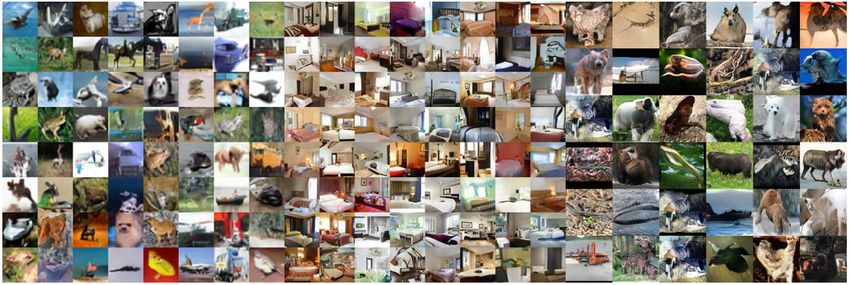
p-blockFigure 6: Randomly generated samples on 32 × 32 CIFAR-10 (left), 64 × 64 LSUN bedroom (middle) and 96 × 96 STL-10 (right) images with ResNet architectures using the proposed method. Evaluation setup details: We used 50000 randomly gen- erated samples comparing against real sets for testing. For each dataset we randomly sampled 50000 images and com- puted FID using 10 bootstrap resamplings. Features were ex- tracted from the pool3 layer of a pre-trained Inception net- work. We display randomly generated examples from un- conditional tasks in Fig 6.
You can also read