Examining the Spatial Distribution of Externalities: Freight Rail Traffic and Home Values in Los Angeles
←
→
Page content transcription
If your browser does not render page correctly, please read the page content below
Examining the Spatial Distribution of Externalities: Freight Rail
             Traffic and Home Values in Los Angeles
                                              Michael Futch∗

                                           November 11, 2011

                                                  Abstract
      This paper measures the impact of infrastructure expansion on local home values and examines
      the persistence of that impact over distance. Specifically, I exploit a natural experiment in which
      rail traffic from the Los Angeles seaport, one of the busiest in the country, was permanently
      redirected from several tracks to a central line, termed the Alameda Corridor. I link a rich,
      repeat-sale housing dataset to plausibly exogenous changes in local rail traffic to estimate these
      effects, controlling for local price trends using a Case-Shiller style housing index. Using the
      actual traffic changes the result is an estimated $3500 decrease in average home value where
      traffic increased and a $1300 increase in average home value where rail traffic was reduced. The
      welfare impact of concentrating a negative externality on a smaller population should depend
      on the convexity of the cost function, but I find evidence that suggests the marginal cost is
      symmetric for winners and losers. Instead, the total welfare impact hinges on the efficiency gains
      achieved by relocating the traffic from circuitous routes to the more direct Alameda Corridor,
      thereby affecting fewer homeowners. While the net gains are minimal, the re-routing of traffic
      resulted in a transfer of housing wealth of approximately $200 million.

   ∗
     Email: mfutch@ucsd.edu. I would like to thank Craig McIntosh, Gordon Dahl, Paul Niehaus, Mark Jacobsen,
Josh Graff Zivin and UCSD seminar participants for their helpful comments.

                                                      1
1 Introduction
Economic reforms often do not benefit everyone involved; instead, there are typically winners
and losers. Identifying who wins and who loses and by how much is important when evaluating
policy options especially because many of the groups affected often do not have representation at
the negotiating table. This process is further complicated when policy actions impact groups or
individuals external to the original intent of the policy.
This is particularly true of public infrastructure projects. Causal identification of public in-
frastructure impact is often challenging as the location is rarely random and may correlated with
wealth and political clout. Using year to year changes in the intensity of an externality is also
problematic as these changes are also likely to be correlated with local growth patterns. When con-
centrating a negative externality on a segment of the population it is important not just to measure
the marginal effect at a point, but to understand the convexity of the cost imposed on individuals.
If the marginal cost of the externality were increasing, this would suggest distributing the exposure
to the externality among as many people as possible. If the marginal cost were decreasing, a case
could be made for concentrating greater amounts of a negative externality on a smaller population.
This paper examines these issues in the context of urban rail in Los Angeles. This setting
offers an attractive natural experiment, solving some of the identification issues discussed above
by exploiting a shift in the way rail traffic travels through the city. The Alameda Corridor, an
urban infrastructure project in Los Angeles, allowed for consolidation of most freight rail traffic
into and out of the San Pedro port facilities from three geographically distinct tracks into one
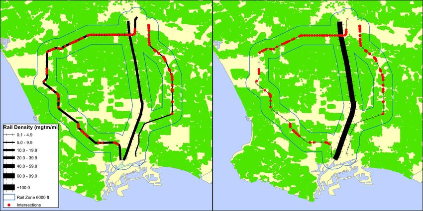
higher capacity line. Figure 1 depicts the level of rail traffic in the region before and after the
opening of the Alameda Corridor. Rail traffic involves negative environmental spillovers onto local
communities in the form of air and noise pollution, along with congestion effects caused by long
waits at rail crossings. Because the rail traffic involved is freight and not transportation, there are
fewer demand-side effects that could cause upward or downward pressure on housing values apart
2Figure 1: Rail Traffic Density - Before and After
from the pollution and congestion caused by rail traffic alone. Most interestingly, the change in the
flow of rail traffic was approximately zero-sum overall, providing a very straightforward window on
the extent to which a redistribution generated net social gains or harm.
This setting allows me to directly measure the distribution of an externality using the cost
inflicted on homeowners, exploiting substantial variation (both upwards and downwards) in the
intensity of the externality. Many papers relate the existence of an externality to house prices,
but most lack the data to clearly identify the costs actually induced by the environmental harm.
I find that an increase in rail traffic by 10 million gross ton miles per mile (MGTM/mi) causes
a 0.7 percentage point lower growth in home values within a 1/3 mile band around the tracks.
Furthermore, under a stronger set of assumptions our results suggest that the response of property
values is linear in the degree of damage in both positive and negative directions for an identical size
change, indicating that a zero-sum redistribution of environmental damage has no overall effect on
total welfare. Using the actual traffic changes this results in an estimated $3500 decrease in average
home value where traffic increased and a $1300 increase in average home value where rail traffic
was reduced. Aggregating our estimates over the number of homes affected yields a net home value
increase of $23 million - a negligible sum considering the total housing value for homes inside the
one-mile zone was roughly $36 billion in 1997.
3The rest of the paper is organized as follows: Section 2 discusses identification strategies and
the data available, Section 3 outlines the estimation strategy and counterfactual selection, Section
4 presents the estimating equations, Section 5 discusses the results, and Section 6 concludes.
2 Identification Strategy and Data
2.1 Causal Identification Issues
While understanding the impacts of public infrastructure on local communities is of much interest,
clean causal identification is typically difficult or impossible in many circumstances. The first
hurdle to causal identification is due to the non-random nature in which locations are chosen
for infrastructure. If the location for a project, say a new railroad track, is chosen based on
unobservable factors that are related to the outcome of interest, OLS estimates of the treatment
effect will be biased. There have been many papers that have taken this approach using cross-
sectional data: Espey and Lopez (2000) and Cohen and Coughlin (2006) both look at the impact
of airport proximity on housing values. Kim, Phipps, and Anselin (2001) use a cross section of
home values and to measure the impact of air pollution on housing prices in South Korea. Chay
and Greenstone (2005) look at air pollution and housing values, but circumvent this identification
hurdle by instrumenting for air pollution using regulation changes triggered by county pollution
levels.
If the housing data available spans several time periods, it could be tempting to use changes
in pollution or changes in the external costs of public infrastructure (greater freeway or airport
traffic) to identify the causal impact on house price changes. However, changes in infrastructure
intensity or air pollution are likely to be correlated with other important variables that may drive
the outcome measure. Greater freeway traffic may negatively impact nearby home values, but that
increased traffic may be a result of higher employment in the city center which could drive up
home prices. If causal effects are to be identified using changes in the externality, an argument
4must be made for the exogeneity of the changes. If the changes are not exogenous, an instrumental
variables or a natural experiment approach could be used if possible. Currie and Walker (2010) use
a repeated cross section data set to exploit the creation of EZ-Pass toll lanes to find the impact of
automobile congestion and poor birth outcomes. The main results of their paper are focused on
health outcomes, but they do look for house price impacts and find none.
A housing data set that includes repeated sales of the same property is especially attractive
once the exogeniety issues have been ironed out. Repeat sale data are useful because they allow
better control of individual house idiosyncrasies. There have been several recent papers that utilize
repeat sale data to estimate the impact of some spatially sourced event. Case et al. (2006) looks
at the effect of water contamination on home prices. Cutter et al. (2009) follow a similar approach
but look at the positive impact of open space preserves on home prices and raise the issue of finding
the appropriate counterfactual. They craft an appropriate counterfactual using matching methods
of Ho, Imai, King, and Stewart (2007). The data Case et al. use has a narrow time window before
the sudden water contamination, so there is little opportunity to gauge the appropriateness of the
counterfactual house trends.
2.2 Natural Experiment
This paper exploits a natural experiment to avoid the common identification pitfalls highlighted
in the previous section. The setting for the natural experiment is freight rail traffic between the
Los Angeles/Long Beach port complex and transfer facilities near downtown Los Angeles about 20
miles away. The Los Angeles and Long Beach seaports rank first and second in terms of container
traffic into and out of the United States and combined comprise the fifth busiest port in the world.
Until recently, much of that traffic passed through the city of Los Angeles on a collection of low
speed rails to reach Union Pacific and BNSF transfer facilities. From there containers continue
on to destinations throughout the United States. In April 2002, the Alameda Corridor opened,
5Figure 2: Bounds on Rail Noise Decay
connecting the port facilities to the rail yards by a more direct and higher capacity track. Also
installed were a series of bridges, trenches, and underpasses at intersections with the purpose of
eliminating more than 200 street level crossings. The goal of the $2.2 billion Alameda Corridor
project was to increase the speed at which cargo travels through the port and to reduce the noise
and traffic congestion caused by slow freight trains at street level. The opening of the Alameda
Corridor should have reduced air and noise pollution in neighborhoods near the tracks through
reduced rail traffic and fewer idling automobiles at railroad crossings. Upper and lower bounds on
the noise decay from train signals are plotted in Figure 2, illustrating the potential noise impact
fading to conversation level after approximately one mile.
The shift in rail traffic induced by the Alameda Corridor was a structural redistribution that
decreased traffic along two of the three main routes between the port and the transfer facilities
increased traffic on the third line. This exogenous redistribution is used to identify the causal
impact of pollution and congestion from freight traffic on local home prices. The spatial shift
can be seen clearly in Figure 1 while the annual changes are plotted in Figure 4. The y-axis in
6Figure 4 is the rail density code indicating the level of rail traffic as reported by the Federal Rail
Administration and the year is on the x-axis. The west and east rails are the non-corridor rails
where traffic decreased, while the center graph shows the sharp spike in traffic on the Alameda
Corridor after the completion of the project.
2.3 Timing of Experiment and Perfect Foresight
Consolidation of the three rails into one higher speed track had been a topic of discussion in Los
Angeles since the early 1980s, but did not become a reality until the late 1990s. Because the
Alameda Corridor required nearly five years of construction before it opened in 2002 it is unlikely
that homeowners near the corridor were taken by surprise when rail traffic skyrocketed after the
opening. Due to the premeditated nature of this intervention, I am likely to see the impact begin
to be capitalized into house prices before the actual opening of the corridor. The housing data
available begin in 1995, before funding was secured or construction commenced, allowing capture
of the full treatment period.
2.4 Housing Data
The housing data from DataQuick include all home sales in ZIP codes within 25 miles of the rails.
The data set includes parcel number, address, sale price, sale date, lot size, bathrooms, bedrooms,
and square feet. The data span the years 1995 to early 2009 and contain nearly 400,000 households
that appear more than once - allowing for creation of a rich panel data set. The data is geolocated
using the address and a streetline GIS file. After geocoding the housing data, a number of additional
variables can be linked to each house including distance from rail lines, proximity to rail crossings,
and Census block/tract.
Table 1 displays summary statistics for housing sales in the different rail zones. A house is
considered to be in a rail zone if it is within one mile of the affected rail. This distance will be
broken out into smaller increments in later analysis. Homes in the rail zones are on average smaller
7Table 1: Home Sale Summary Statistics: 1995-2009
Sales Price Sq. Feet Beds Baths
Corridor Zone 10,991 171,705 1,165 2.67 1.46
West Rail Zone 33,222 276,197 1,392 2.80 1.89
East Rail Zone 19,634 208,478 1,246 2.64 1.63
Greater LA 519,258 356,324 1,582 2.84 2.05
Table 2: Difference-in-Difference Estimates
One Mile Bands Incremental Bands DID
Log Price in Corridor Before 11.68 Corridor 0 - 1/3 mile -0.033
Log Price in Corridor After 12.29 (0.015)**
Difference 0.61 Corridor 1/3 - 2/3 mile -0.025
Difference-in-Difference w/ LA -0.018 (0.013)**
Standard Error on DID (0.008)** Corridor 2/3 - 1 mile -0.002
(0.013)
Log Price in Non-Corridor Before 12.03 Non-Corridor 0 - 1/3 mile 0.034
Log Price in Non-Corridor After 12.67 (0.010)***
Difference 0.64 Non-Corridor 1/3 - 2/3 mile 0.002
Difference-in-Difference w/ LA 0.013 (0.009)
Standard Error on DID (0.006)** Non-Corridor 2/3 - 1 mile 0.012
(0.009)
Log Price in LA Before 12.32
Log Price in LA After 12.95
Difference 0.627
Standard Error on Difference (0.002)***
and less expensive compared to homes in the rest of the city. Among the rail zones, the homes
around the Alameda Corridor tend to be the smallest and least expensive. The differences in value
and size of the homes in different zones highlight the need for care in controlling for localized price
trends. As motivation for further study of home price trends in the rail zones we provide a simple
difference-in-difference in Table 2. This table shows that the prices for homes within a mile of the
Alameda Corridor, where rail traffic increased considerably, grew about 1.8 percent slower than
homes in the rest of Los Angeles. The negative effect was also stronger for homes closest to the
rail as can be seen when the one mile zone is broken into increments. For homes nearest to the
non-corridor rails, where traffic was decreased, home prices outpaced the rest of Los Angeles by 1.3
percent. Again, the effect is strongest for homes nearest to the rail. Using the rest of Los Angeles
as the counterfactual may not be correct and this will be explored later, but the simple difference
in difference result motivates further inquiry.
8Figure 3: Los Angeles HPI (1995=100)
2.5 Housing Boom and Bust
The period under examination here contains the growth and subsequent popping of the house price
bubble in the United States. Home prices in Los Angeles were not exempted from this phenomenon
in the slightest. Figure 3 shows the rapid price growth witnessed in Los Angeles during the late
1990s and early 2000s and an equally rapid decline in prices when the bubble burst in 2006. The
volatile nature of home prices during this period is even more reason to be careful when choosing
a counterfactual set. Additionally, we want to be sure that our estimates are not being driven by
the unusual events of the time period. We will report estimates that include the entire time period,
boom and bust, and as a robustness check we restrict the sample to the period directly after the
opening of the Alameda Corridor and drop transactions that occurred during the crash.
2.6 Rail Traffic Data
Rail traffic data are provided by the National Transportation Atlas published by the Bureau of
Transportation Statistics. The data include a GIS map of the rail network along with a categorical
measure of rail traffic density for each rail segment from 1995 to 2006. Rail density is a measure of
the gross ton-miles of cargo traveled over a section of rail, divided by the length of the rail segment.
9Figure 4: Annual Rail Traffic Density
For example, if a 100 mile track had only one gross ton of cargo traveling its length it would have
a density of one gross ton mile per mile. A shorter track with the same number of gross ton miles
would clearly have a much higher density. While not a perfect measure of the number of trains
traveled, we believe it is an excellent proxy.
3 Estimation Strategy
3.1 Repeat Sale Framework
To estimate the causal impact of an increase in rail traffic on local home values we begin with the
assumption that home prices follow a hedonic price function:
pi,t = αi + τt + βDENi,t ∗ P roximityi + η 0 xi + ui,t (1)
where pi,t is the log price of home i at time t, τt is the local home price index at time t, DENi,t is
the rail density of the nearest rail interacted with some indicator for proximity to the rail, and xi is
a vector of home characteristics. Because our data contain repeated observations we can difference
this equation with its previous sale, eliminating individual home idiosyncrasies and giving us the
10following equation:
∆pi,t = ∆τt + β∆DENi,t ∗ P roximityi + vi,t (2)
The term ∆τ represents the change in the local house price index between time t and the
period in which the home was last sold. In order to estimate β we will need to first identify the
appropriate counterfactual group, then use the methods pioneered by Case and Shiller (1987) to
estimate local house price trends and find fitted values ∆τ
dt for each home sale. If a home was sold
in 1995Q2 and again in 1999Q4, the fitted value for ∆τ for that home will yield the expected price
change for a home that sold in those time periods if the rail traffic pattern had not changed. The
xi could contain time-varying characteristics capturing home remodels or additions, though our
housing characteristic data are limited in this respect and do not vary over time.
3.2 House Price Index Calculation
To control for counterfactual price changes and to evaluate whether a set is an appropriate counter-
factual we estimate Case-Shiller style house price indices. Standard repeat sale estimation begins
with log home price as the dependent variable and an indicator for time period sold on the right
hand side of the equation.
Pi = γ + τ1 Ti,1 + ... + τn Ti,n + ui (3)
We arrive at the estimating equation by taking a first difference:
∆Pi = τ1 ∆Ti,1 + ... + τn ∆Ti,n + vi (4)
so that a home sold first in period s and subsequently in period t would have a value of 1 for
∆Ti,t and a value of -1 for ∆Ti,s . The predicted log price change would then be given by τˆt − τˆs
11or, fitting with earlier notation, ∆τt . The τ coefficients are estimated using GLS, applying the
standard heteroskedasticity correction for differing lengths of time between sales.
3.3 Selection of Counterfactual Set
Measuring the impact of rail traffic on housing prices requires an appropriate counterfactual to
control for local price trends. House price trends are location specific, so the overall trend in a city
or region may not be a good predictor of changes in a neighborhood. Other approaches have used
matching methods to create a counterfactual group that resembled the affected homes in physical
attributes. The approach taken here is to create a house price index (HPI) using homes that closely
follow the pre-treatment trend in the rail zones, but are outside the one mile radius that we use to
define the rail zone. The house price index can then be used to generate predicted values for the
expected price change.
To find an appropriate counterfactual for homes in the affected rail zones we first compare the
house price index for Los Angeles in general with the indices generated by homes in each zone.
This is accomplished by running the standard repeat sale estimation equation and also interacting
the housing index regressors with indicators for the relevant zone. If homes in each zone follow the
same house price trend as the rest of the city, the difference in coefficients for each time period
before the treatment should be insignificant. These differences are plotted for each zone in Figure
5. Panel (a) shows the difference between HPI coefficients for the west zone versus those for the
rest of Los Angeles, panel (c) shows the same difference but for homes in the east zone, and finally
panel (e) shows the differences for the corridor zone versus the rest of Los Angeles. Each of the
three zones show statistically different house price index coefficients from Los Angeles as a whole.
This is especially true for the east and corridor zones in panels (c) and (e). This indicates that
using home prices for the rest of Los Angeles is not going to provide the correct counterfactual
changes.
12As an alternative to using city-wide trends as the counterfactual, we propose using homes in
the ”marginal” rail zone, homes one to two miles from each affected rail. To test the validity of
this counterfactual group we follow the same method as before. The difference in coefficients for
each zone and its marginal zone are plotted in panels (b), (d), and (f) of Figure 5. In each case
the HPI coefficients are statistically indistinguishable from those for the accompanying marginal
zone - confirming that the marginal zones are indeed providing the correct counterfactual changes.
For the remainder of the paper, the marginal zones around each rail will be used to produce fitted
values to control for counterfactual changes in the absence of the rail shift, though using the city
of Los Angeles as the counterfactual instead does not fundamentally alter the results.
4 Estimation
This section presents the basic estimation equations for measuring the impact of rail traffic density.
While the rail traffic density decreased in the east and west zones and increased in the corridor zone,
the coefficients on each density change regressor below are all expected to be negative reflecting
the disamenity value of rail traffic in a neighborhood. The magnitude of the coefficients should be
decreasing in absolute value as the distance from the rail increases, as homes further from the track
are likely to experience lower noise, pollution, and congestion. In each specification below, the log
price change for a home is regressed on the change in rail density, the predicted house price based
on the relevant WRS index, and a vector of seasonal and neighborhood dummies. The method for
choosing a predicted house price will be addressed in the following section.
4.1 Model 1 - Baseline
The first model examines the impact of the rail traffic changes in 1/3 mile-incremental bands around
each affected rail without distinguishing between the Alameda Corridor and the other two rails.
The assumption that all rail traffic affects home prices in the same way will be relaxed in later
13Figure 5: HPI Coefficient Differences and 95% Confidence Bands on Point Estimates
(a) West vs. LA (b) West vs. Marginal West
(c) East vs. LA (d) East vs. Marginal East
(e) Corridor vs. LA (f) Corridor vs. Marginal Corridor
14analysis.
3
X
∆Pi = γ ∆P
di + ψj ∆DENi ∗ AnyRailj,i + β 0 xi + ui
j=1
The format for regressors indicating the zone in which the house is located is as follows:
1 if Distance (mi) to Rail ∈ (0, .33)
AnyRail1,i =
0 otherwise
1 if Distance (mi) to Rail ∈ (.33, .67)
AnyRail2,i =
0 otherwise
1 if Distance (mi) to Rail ∈ (.67,1)
AnyRail3,i =
0 otherwise
4.2 Model 2 - Railroad Crossing Increments
The second specification includes an indicator for proximity to railroad crossings. Federal law
requires trains to sound their horn when approaching street crossings, which is likely to augment
the already negative impact of train traffic through a neighborhood. Train signals are required to be
heard between 96 and 110 dB from a distance of 100 feet. Figure 2 displays lower and upper bounds
on the sound decay of a train signal as you move further away from the track. Because the Alameda
Corridor was constructed using a series of trenches and bridges, railroad crossings only exist on
the east and west rail lines. This model divides the intersection zone into 500 foot increments to
explore how the impact of rail density evolves with distance around these intersections. Each home
in the intersection crossing zone will also be located in the zone closest to the rail, so the full effect
of a density change for these houses will be the sum of ψ1 and λ. As with the incremental zone
variables, the impact of the traffic change at an intersection is expected to fade with increased
distance.
153
X 3
X
∆Pi = γ ∆P
di + ψj ∆DENi ∗ AnyRailj,i + λj ∆DENi ∗ (Crossingj,i ∗ AnyRail1,i )+
j=1 j=1
β 0 X̄i + ui
4.3 Model 3 - Heterogeneous Rail Traffic Impacts
Part of the intent for the Alameda Corridor was to move containers through the city without the
need for rail crossings. This was accomplished through a series of bridges, trenches and underpasses.
To allow for heterogeneous impacts from rail traffic density, the previous two models are expanded
to distinguish between corridor and non-corridor rail traffic. The non-corridor traffic will be further
disaggregated by geography.
3
X 3
X
∆Pi = γ ∆P
di + ψj ∆DENi ∗ N onCorrj,i + φj ∆DENi ∗ Corridorj,i +
j=1 j=1
3
X
λj ∆DENi ∗ Crossingj,i + β 0 X̄i + ui
j=1
5 Results
5.1 Locally Weighted Regressions
Before presenting the full regression results, inspection of Figure 6 helps to motivate the more
detailed study. In each figure, the unexplained price change is non-parametrically regressed on
the distance from the rail for home sale pairs both before and after the opening of the Alameda
Corridor. The unexplained price change is found by taking the actual log price change less the
predicted price change using the appropriate ”marginal” rail zone discussed above. Panels (a)
and (c) include homes within one mile of the rails where traffic was drastically reduced. Homes
closest to the rail that were sold before the change in rail traffic grew in price about 10 percent
less than expected, an effect that gradually fades toward zero as the distance increases, at least
for the westernmost rail. The price-distance pattern is clearly different for the homes sold after
the rail change. Homes close to the rail sold for more than expected and as the distance from the
16.1
-.1
-.2
-.3
.3
.2
.1 5Non-Corridor
43210Unexplained Price Change West
(Log) Rail .1istance fromCorridor
-.1
-.2
-.3
.3
.2 Alameda
5D
Distance
Before
After
43210.1 Rail in ft (000s) .1
-.1
-.2
-.3
.3
.2 Non-Corridor
543210.1 East Rail
Non-Corridor West Rail Alameda Corridor Non-Corridor East Rail
.3
.3
.3
Before
After
Unexplained Price Change (Log)
.2
.2
.2
.1
.1
.1
0
0
0
-.1
-.1
-.1
-.2
-.2
-.2
-.3
-.3
-.3
0 1 2 3 4 5 0 1 2 3 4 5 0 1 2 3 4 5
Distance from Rail in ft (000s)
(a) Non-Corridor West Rail (b) Alameda Corridor Zone (c) Non-Corridor East Rail
Figure 6: Locally Weighted Distance Regressions
rail increases the difference between the actual and expected price change falls toward zero. These
patterns give evidence that the rail change was not anticipated by home buyers in the rail zone
and that the redirection of traffic has given a noticeable boost to home prices close to the rail,
eventually fading as you get further from the line.
The plot in panel (b) shows the same non-parametric regression but for the homes around the
Alameda Corridor itself where rail traffic was significantly increased. Regardless of whether it was
sold before or after the opening of the corridor, homes closer to the corridor sold for less than
expected. The gap between sale price and expected sale price narrows for homes located further
from the corridor both before and after the opening, which fits with the idea that the impact of the
rail traffic should die off with distance. The similar price-distance pattern for homes sold before and
after indicates that prices in the corridor area were negatively impacted before the corridor opened.
With an infrastructure project of this scale, it is not surprising at all that prospective home buyers
and sellers in the area were aware of the potential impact. The fact that the pattern persisted even
after the opening suggests that the negative impact of the rail traffic was not completely capitalized
into home prices beforehand.
175.2 Basic Model Results
The regression results for the first two models described earlier are summarized in Table 3. The
units of the rail density measure in these regressions are hundred millions of gross ton miles per
mile. In Panel A, the first column does not include zone or seasonal dummy variables or any
housing characteristics, only the density change of the nearest rail interacted with the indicator for
which zone in which the home is located. Column I shows a strong negative effect of an increase
in the rail density for the homes within 1/3 of a mile of a rail. This indicates that for these homes,
an increase in rail density of 100 million gross ton miles per mile will cause home prices in the area
to fall by -0.6 percent. While this may seem small, the re-routing of traffic due to the Alameda
Corridor increased traffic in the corridor zone by 50 to 90 million gross ton miles per mile. The
negative effect of a density increase is lessened, but still statistically different from zero, for the
next set of homes 1/3 to 2/3 of a mile from the rail. A one unit increase in rail density causes a
-0.3 percent fall in the home price in this zone. Finally, for homes between 2/3 of a mile and one
mile from the track the negative effect disappears. The coefficient for this last group is small and
positive, but not significant. Column II includes zone indicators for all homes, seasonal dummies,
and housing characteristics. All coefficients move towards zero and the standard errors are larger,
but the overall pattern where the impact diminishes with distance remains.
Column III introduces indicators for proximity to a rail crossing interacted with the rail density
change. The coefficient on density change for homes nearest an intersection (within 500 ft) is
considerably more negative than for the rest of the zone but is not statistically significant. The
period under study can be considered to be anomalous as the growth and subsequent popping of
the real estate bubble characterizes the second half of the housing data. As a robustness check,
Column IV restricts the data set to homes sold before the crash in housing prices. Truncation of the
data pushes the coefficient on density change for homes nearest a crossing further negative. Since
traffic was falling at these intersections we can interpret this result to mean the housing bubble
18likely sapped some of the price boost felt by homes in this area.
Thus far it has been implicitly assumed that homebuyers and sellers are myopic about the
impact of the Alameda Corridor on home values. This assumption is especially strong for homes
near the corridor itself, as construction spanned several years and was by no means a minor project.
Ideally it would be possible to use a timeline of the corridor’s construction or news stories about
the planning of the corridor as the points in time when agents became aware of the potential
home price impacts. Unfortunately, the housing data available for this paper begin in 1995 and
planning for the corridor began in the early 1980s. Instead I exclude homes that were sold during
the construction period of the corridor and report the results in Panel B of Table 3. Despite the
reduction in observations, the coefficients do not change much and are more precisely estimated.
5.3 Heterogeneous Effects
The regressions above were re-run to allow the coefficients on rail density to differ for corridor and
non-corridor traffic. We see in Table 4 the pattern of negative impacts dissipating with distance
persists, but the coefficients for corridor traffic are larger and more precisely estimated. For homes
in the zone closest to the non-corridor rails, a 10 MGTM/mi increase in density causes a -0.5
percent decline in home prices. However, rail traffic in these areas fell so homes were appreciating
at a faster pace than expected. The impact of a density change in the next zone around non-corridor
rails is negative, but only statistically different from zero if the housing crash is excluded. In the
corridor zone a 10 MGTM/mi increase in density causes a -0.8 percentage point lower growth than
expected. This translates to a 4 percent lower home price growth when rail traffic increased by 50
MGTM/mi.
It should be noted that, while they are not statistically different, it is somewhat unexpected that
the coefficient on corridor traffic is larger in absolute value. My expectation was that the coefficient
would be smaller, capturing the concavity created by diminishing effect of greater amounts of traffic
19Table 3: Impact of Rail Traffic on Home Prices
Panel A - Includes Construction Period Panel B - Excludes Construction Period
Log Price Change Log Price Change
I II III IV I II III IV
∆ Rail Traffic: Baseline Covariates Intersections No Crash Baseline Covariates Intersections No Crash
0 - 1/3 mi. from Any -0.062 -0.050 -0.032 -0.024 -0.062 -0.049 -0.016 -0.008
(0.010)*** (0.022)** (0.026) (0.039) (0.015)*** (0.018)*** (0.020) (0.027)
1/3 - 2/3 mi. from Any -0.035 -0.044 -0.051 -0.086 -0.039 -0.051 -0.063 -0.111
(0.012)*** (0.020)** (0.018)*** (0.019)*** (0.014)*** (0.020)** (0.022)*** (0.027)***
2/3 - 1 mi. from Any 0.019 0.010 0.004 -0.020 0.025 0.018 0.006 -0.029
(0.018) (0.011) (0.026) (0.023) (0.014)* (0.015) (0.014) (0.020)
500 ft from Crossing -0.248 -0.298 -0.286 -0.353
20
(0.169) (0.121)** (0.105)*** (0.107)***
1000 ft from Crossing -0.015 -0.010 -0.067 -0.076
(0.059) (0.071) (0.066) (0.074)
1500ft from Crossing -0.040 -0.082 -0.079 -0.122
(0.076) (0.080) (0.070) (0.077)
Zone Indicators No Yes Yes Yes No Yes Yes Yes
Housing Characteristics No Yes Yes Yes No Yes Yes Yes
Seasonal Indicator No Yes Yes Yes No Yes Yes Yes
Observations 28586 28586 28586 20578 24833 24833 24833 17675
R-squared 0.8518 0.8536 0.8537 0.8283 0.8339 0.8358 0.8358 0.8058
Bootstrapped standard errors in parentheses
* significant at 10%; ** significant at 5%; *** significant at 1%- a hypothesis that will be tested later. One possible explanation is that homeowners and sellers
surrounding the non-corridor rail were better informed as to the impact of the rails, they could
have acted on this information prior to the redirection of traffic, dampening the total effect. Under
this circumstance, excluding the construction period should bring the estimates for each zone closer
together, which we can see in Panel B is the case.
Once construction period homes are excluded, we find that rail density changes have similar
impacts for homes in the first two zones around corridor and non-corridor rails. While the impact
of density changes for the first two zones are similar, the effect dies out faster for non-corridor
homes. Homes located between 2/3 of a mile and one mile from the Alameda Corridor still felt
a negative impact, falling -0.2 percent for each additional 10 MGTM/mi. However, homes that
are the same distance from non-corridor rails do not experience a measurable impact from a rail
change. Whether using Panel A or B, the strength of the density effect is greatly magnified for
homes in the immediate vicinity of rail road crossings. Rail density in this area fell from about 30
MGTM/mi to 2.5 MGTM/mi meaning homes nearest the rail grew about 8.3 percent above the
expected price.
When the non-corridor traffic is disaggregated even further (Table 5), separating the rail west of
the corridor from the rail to the east, we find that the effect of the rail density change is concentrated
around the railroad crossings and is stronger in the west. In fact, there is no effect for homes around
the east railroad unless located near an intersection. The coefficient on density change for homes
nearest to an east intersection should be disregarded as very few homes are located in this zone and
even fewer (16) have sale pairs spanning a density change. These coefficients for rail crossing homes
are negative, but only significant if we consider home sales before the housing bust, suggesting that
any stronger growth felt in the area was given back when housing prices began falling. There are
two possible explanations for the weaker results along the east rail. First, if container traffic from
the port does not leave on rail, it leaves on trucks. Interstate 710 is the major truck route leaving
21Table 4: Impact of Rail Traffic on Home Prices: Heterogeneous Impacts
Panel A - Includes Construction Period Panel B - Excludes Construction Period
Log Price Change Log Price Change
I II III IV I II III IV
∆ Rail Traffic: Baseline Covariates Intersections No Crash Baseline Covariates Intersections No Crash
0 - 1/3 mi. from Non-Corridor -0.050 -0.037 0.005 0.000 -0.068 -0.058 -0.006 -0.007
(0.029)* (0.023) (0.030) (0.046) (0.027)** (0.024)** (0.036) (0.045)
1/3 - 2/3 mi. from Non-Corridor -0.023 -0.033 -0.032 -0.073 -0.042 -0.056 -0.056 -0.108
(0.019) (0.026) (0.032) (0.026)*** (0.028) (0.027)** (0.029)* (0.038)***
2/3 - 1 mi. from Non-Corridor 0.032 0.022 0.022 -0.007 0.023 0.013 0.013 -0.025
(0.017)* (0.019) (0.024) (0.025) (0.020) (0.021) (0.020) (0.031)
0 - 1/3 mi. from Corridor -0.080 -0.088 -0.088 -0.138 -0.071 -0.076 -0.076 -0.148
(0.016)*** (0.013)*** (0.024)*** (0.036)*** (0.015)*** (0.022)*** (0.022)*** (0.030)***
1/3 - 2/3 mi. from Corridor -0.065 -0.056 -0.056 -0.056 -0.068 -0.063 -0.063 -0.059
(0.014)*** (0.020)*** (0.018)*** (0.024)** (0.014)*** (0.014)*** (0.022)*** (0.021)***
22
2/3 - 1 mi. from Corridor -0.035 -0.033 -0.033 -0.062 -0.024 -0.027 -0.027 -0.040
(0.013)*** (0.016)** (0.016)** (0.020)*** (0.013)* (0.017) (0.020) (0.022)*
500 ft from Crossing -0.276 -0.314 -0.290 -0.349
(0.122)** (0.183)* (0.113)*** (0.111)***
1000 ft from Crossing -0.044 -0.026 -0.072 -0.071
(0.069) (0.083) (0.058) (0.065)
1500 ft from Crossing -0.069 -0.098 -0.084 -0.117
(0.044) (0.084) (0.066) (0.083)
Zone Indicators No Yes Yes Yes No Yes Yes No
Housing Characteristics No Yes Yes Yes No Yes Yes No
Seasonal Indicator No Yes Yes Yes No Yes Yes No
Observations 28586 28586 28586 20578 24833 24833 24833 24833
R-squared 0.8520 0.8537 0.8538 0.8283 0.8341 0.8359 0.8359 0.8059
Bootstrapped standard errors in parentheses
* significant at 10%; ** significant at 5%; *** significant at 1%the port and cuts directly through the east rail, so it is possible that rail traffic has been substituted
for truck traffic in this area; something that could be explored further. Additionally, the homes in
the most densely populated area of the east rail zone are also located adjacent to the rail yards
where idling train have created a health risk for neighboring communities (ARB 2007). For the
west rail, the coefficients are comparable to the earlier estimates, but the precision is reduced. If
the construction period is excluded, we get the familiar pattern of a strong negative effect of rail
density that diminishes as you move further from the rail.
5.4 Convexity of Costs
The nature of traffic shift that occurred due to the Alameda Corridor offers an opportunity to
explore how homeowners react to differing levels of an externality. Homeowners along the corri-
dor were faced with sharp increases in rail traffic near their homes, while homes in other areas
experienced a sharp decline in traffic. This tandem upward and downward shift allows us to gain
some insight into the marginal cost structure associated with the intensity of this externality. If
the marginal cost of an increase in traffic is different in absolute value than the marginal cost of
a decline in traffic the welfare implications of rail traffic will hinge on where these burdens are
borne. Consider a situation where two equally populated neighborhoods each had a track running
through. If the marginal cost of traffic were increasing total welfare would be largest with an equal
distribution of traffic. However, if the marginal cost were diminishing an argument could be made
that one of the neighborhoods should carry the traffic and could be compensated in some way by
the other. If the marginal cost were constant, distribution of the traffic would be less important as
it does not impact the magnitude of the welfare impact.
The test we perform to determine whether marginal costs are increasing or decreasing is to
use a approximation to the marginal cost and compare the regression coefficients for a change in
density in the corridor zone versus the non-corridor zone. Because the the areas have different
23Table 5: Impact of Rail Traffic on Home Prices: Disaggregated Zones
Panel A - Includes Construction Period Panel B - Excludes Construction Period
Log Price Change Log Price Change
I II III I II III
∆ Rail Traffic : Baseline Covariates Intersections No Crash Baseline Covariates Intersections No Crash
0 - 1/3 mi. from Non-Corridor West -0.069 -0.063 -0.027 -0.030 -0.098 -0.088 -0.046 -0.050
(0.039)* (0.038)* (0.045) (0.060) (0.040)** (0.041)** (0.064) (0.066)
1/3 - 2/3 mi. from Non-Corridor West -0.035 -0.051 -0.051 -0.102 -0.063 -0.079 -0.078 -0.155
(0.030) (0.029)* (0.039) (0.048)** (0.032)** (0.040)* (0.033)** (0.042)***
2/3 - 1 mi. from Non-Corridor West 0.022 0.014 0.015 0.000 0.016 0.012 0.012 -0.024
(0.029) (0.024) (0.031) (0.035) (0.033) (0.041) (0.032) (0.045)
0 - 1/3 mi. from Non-Corridor East -0.012 0.009 0.034 0.021 -0.009 0.011 0.045 0.040
(0.050) (0.031) (0.050) (0.069) (0.052) (0.033) (0.042) (0.049)
1/3 - 2/3 mi. from Non-Corridor East 0.004 0.000 -0.000 -0.028 0.005 0.001 0.000 -0.019
(0.038) (0.037) (0.047) (0.037) (0.059) (0.042) (0.043) (0.040)
2/3 - 1 mi. from Non-Corridor East 0.051 0.035 0.035 -0.026 0.043 0.032 0.032 -0.020
(0.036) (0.036) (0.039) (0.024) (0.044) (0.031) (0.035) (0.050)
0 - 1/3 mi. from Corridor -0.080 -0.087 -0.087 -0.139 -0.070 -0.071 -0.071 -0.147
(0.015)*** (0.013)*** (0.025)*** (0.035)*** (0.017)*** (0.023)*** (0.022)*** (0.028)***
24
1/3 - 2/3 mi. from Corridor -0.065 -0.055 -0.055 -0.058 -0.067 -0.059 -0.059 -0.057
(0.015)*** (0.019)*** (0.019)*** (0.026)** (0.018)*** (0.016)*** (0.021)*** (0.022)**
2/3 - 1 mi. from Corridor -0.035 -0.032 -0.032 -0.063 -0.022 -0.022 -0.022 -0.039
(0.016)** (0.017)* (0.016)** (0.020)*** (0.010)** (0.018) (0.019) (0.023)*
500 ft from West Crossing -0.275 -0.325 -0.275 -0.344
(0.137)** (0.228) (0.143)* (0.138)**
1000 ft from West Crossing 0.004 0.045 -0.015 0.009
(0.090) (0.096) (0.066) (0.088)
1500 ft from West Crossing -0.050 -0.047 -0.055 -0.059
(0.071) (0.110) (0.083) (0.099)
500 ft from East Crossing -0.120 0.123 -0.129 0.091
(0.232) (0.483) (0.273) (0.480)
1000ft from East Crossing -0.124 -0.219 -0.151 -0.251
(0.136) (0.116)* (0.168) (0.144)*
1500 ft from East Crossing -0.061 -0.184 -0.084 -0.197
(0.085) (0.064)*** (0.087) (0.100)**
R-squared 0.8520 0.8537 0.8539 0.8283 0.8341 0.8359 0.8361 0.805
Observations 28586 28586 28586 20578 24833 24833 24833 17675
Bootstrapped standard errors in parentheses
* significant at 10%; ** significant at 5%; *** significant at 1%home values we will need to incorporate this difference into the test in order to find the marginal
dollar cost. Additionally, to test convexity of the cost structure some stronger assumptions have
to be made. I am forced to assume that an increase in rail traffic in each area causes the same
level of negative impact and that the difference in how it is capitalized into home prices is due to
individuals preferences over these impacts. This may be a difficult assumption to accept as the
Alameda Corridor was constructed such that trains would no longer cross streets at surface level.
Removing traffic from surface level interactions is likely to reduce the impact that homeowners
perceive, so our test is possibly biased towards accepting the hypothesis that marginal costs are
diminishing. The hypothesis test is as follows:
H0 : ψ1 AvgP riceN onCorridor1 = θ1 AvgP riceCorridor
(5)
H1 : ψ1 AvgP riceN onCorridor1 > θ1 AvgP riceCorridor
Using estimates from Table 4 we fail to reject the null hypothesis that marginal costs are
constant. The coefficients on density change are similar or higher in the corridor zone, but the
average home value is higher in the non-corridor zone. A change of 10 MGTM/mi in rail density
causes a change in home value of $1,180 in the western non-corridor zone, $863 in east rail zone,
and a $832 change in home value in the corridor zone. The difference between these estimates is
not statistically significant at any conventional level. While this test is imperfect due to the strong,
and possibly invalid, assumptions required, it does still provide some evidence against diminishing
marginal cost of the externality as the test is biased in the direction of finding diminishing marginal
costs, but finds no evidence of this. Performing a joint test of the hypothesis that the marginal
effects for each distance band are the same between corridor and non-corridor rails brings us to the
same conclusion.
25Figure 7: Household Density
!
!
! !
!
! !
!
!
!!!!!!!!!!!!!!
!!!!!!!
!!! !
!! !
!!
!!! !
!! !
!
!
!!! !!! !!
!! !
!!
!
! !
!
!
! !
!
! !
!
! !
!
!
!
!
!
! !
!
!
!
!
!
!
!
!!
!!
!
!! !!
!!
Households per Sq. Mi.
Census Blocks 2000
1 - 2202
2203 - 4887
4888 - 9389
9390 - 17370
17380 - 41620
5.5 Aggregating Impact
If the population density and distance of each affected line were identical we would only need
the marginal effect and density change to determine whether the net effect capitalized into home
prices was positive or negative. As can be seen in Figure 7, the population density is not constant
along each line and, in fact, there are very few homes near the lower section of the central Alameda
Corridor. In addition to changing population densities, the length of each line differs. To understand
how this affects the overall impact of the rail shift, we must tabulate the number of homes and
the average price in each zone. Using Census 2000 data we find the number of housing units in
each Census block and using our housing data we find the average pre-treatment price. Using this
information and the marginal effects calculated in the earlier regressions we can add up the total
impact capitalized into home prices. Figure 8 displays number of housing units affected on the
x-axis, sorted by distance to a rail, and the cumulative impact on the y-axis with the negative
and positive impacts plotted separately. In panel (a) we use the regression coefficients from Panel
B Column II of Table 5 to estimate the total effect on housing, finding the positive impact to be
26Figure 8: Cumulative Impact of Rail Shift
(a) Disaggregated Impacts (b) Intersections
300
250
200
150
100
50
Cumulative
5
0
50000
100000
150000
200000
Number
Positive
Negative
0
0000 Impact
ofImpact
Housing
Cost/Benefit
300 Units (Sorted by Distance) 300
250
200
150
100
50
Cumulative
5
0
50000
100000
150000
200000
Number
Positive
Negative
0
0000 Impact
ofImpact
Housing
Cost/Benefit
Units (Sorted by Distance)
300
250
250
Cumulative Cost/Benefit
Cumulative Cost/Benefit
200
200
150
150
100
100
50
50
0
0
0 50000 100000 150000 200000 0 50000 100000 150000 200000
Number of Housing Units (Sorted by Distance) Number of Housing Units (Sorted by Distance)
Positive Impact Negative Impact Positive Impact Negative Impact
roughly $23 million greater than the negative impact. It should be noted that line for the negative
impact is more steeply sloped, not because of a difference in the marginal effect, but because the
change in rail traffic was greater on the Alameda Corridor than on the individual non-corridor
rails. Finally, when we use the most detailed specification including the effect on homes around
the railroad crossings we see in panel (b) that the positive impact is now steeper initially due to
the magnified effect around the rail crossings and that the gap between the positive impact and
negative impact is wider. Considering the magnitude of the housing value in the one-mile zone
around the rails totaled $36 billion in 1997, the small total positive impact is negligible. While
the net impact may be negligible, there has been a significant transfer of housing value from the
communities surrounding the Alameda Corridor, which tend to be predominantly minority and
lower income, to higher income neighborhoods surrounding the non-corridor rails.
6 Conclusion
This paper exploited a natural experiment to measure the positive and negative impacts of rail
traffic on neighboring homes. I find strong evidence negative spillovers from local rail traffic nega-
27tively impact home values. Additionally, the case for concentration of a negative externality is not
supported as I did not find evidence of concavity or convexity of the cost of rail traffic on homes.
Therefore a zero-sum redistribution of traffic would be expected to have no impact. In this case,
there was a small positive impact on housing values as a result of the more direct routing of traffic.
Because the Alameda Corridor saw a larger increase in absolute value than the decrease on the
other lines, the negative impact felt by a home along the Alameda Corridor was greater in absolute
value than the positive impact received by a home along a rail where traffic was reduced. However,
there were many more homes along the non-corridor rails leading to the small net positive effect.
The positive gain was muted by the narrowly focused impact felt around the eastern non-corridor
rail. Because of the confounding effect of the 710 interstate and nearby inter-modal railyards, the
positive benefit was confined to the homes near rail crossings.
The rail traffic setting explored here is ideal for investigating the negative externality effects
of infrastructure expansions with little interference from demand side effects. If the re-routing
experiment had been for highway or airport traffic the negative impacts would have been more
difficult to measure as the positive effects of proximity to airports or reduced commute times would
have likely influenced home values. The use of freight rail traffic allowed for cleaner estimation of
this impact. The most likely source of this type of demand side impact from freight rail would
be from greater employment opportunities during construction, though the longer window of data
available allows this issue to be circumvented.
Infrastructure expansions are often touted as local job creators, but there are also costs borne by
the localities. Understanding the spatial dispersion of the costs and whether there are convexities
is necessary when evaluating these projects. From this paper, the lack of evidence of diminishing
marginal cost suggests that concentrating the negative impacts of an infrastructure project yield no
reduction in the welfare costs. The fact that we uncover a relatively linear marginal damage curve
for winners and losers from this infrastructural redistribution indicates that there are no complex
28welfare dynamics at work, at least as revealed by home prices. This would indicate that planners
considering future projects will maximize welfare simply by making transportation infrastructure
as direct and efficient as possible when local impacts are unavoidable.
References
[1] Case, Colwell, Leishman, and Craig Watkins (2006), The Impact of Environmental Contamina-
tion on Condo Prices: A Hybrid Repeat-Sale/Hedonic Approach, Real Estate Economics, Vol.
34, 77-107.
[2] Case, Karl and Robert Shiller (1987), Prices of Single Family Homes Since 1970: New Indexes
for Four Cities, New England Economic Review, September-October, 46-56.
[3] Chay, Kenneth Y. and Michael Greenstone (2005), Does Air Quality Matter? Evidence from
the Housing Market, Journal of Political Economy, Vol. 113 No. 2, 376-424.
[4] Cohen, Jeffery P. and Cletus C. Coughlin (2008), Spatial Hedonic Models of Airport Noise,
Proximity, and Housing Prices, Journal of Regional Science, Vol. 48 Issue 5, 859-878.
[5] Currie, Janet and Reed Walker (2010), Traffic Congestion and Infant Health: Evidence from
E-Z Pass, American Economic Journal: Applied Economics, Vol. 3 No. 1 January 2011, 65-90.
[6] Cutter, Fernandez, Sharma, and Thomas Scott (2009), Dynamic Analysis of Open Space Value
Using a Repeat Sales/Hedonic Approach, Working Paper.
[7] Espey, Molly and Hilary Lopez (2000), The Impact of Airport Noise and Proximity on Residen-
tial Property Values, Growth and Change, Vol. 31 Issue 3, 408-419.
[8] Ho, Imai, King and Elizabeth A. Stuart (2007), Matching as Nonparametric Preprocessing for
Reducing Model Dependence in Parametric Causal Inference, Political Analysis, Vol. 15 Issue
3, Summer, 199-236.
29[9] Kim, Phipps, and Luc Anselin (2003), Measuring the Benefits of Air Quality Improvement: A
Spatial Hedonic Approach, Journal of Environmental Economics and Management, Vol. 45 Issue
1, 24-39.
[10] Rosen, Sherwin (1974), Hedonic Prices and Implicit Markets: Product Differentiation in Pure
Competition, Jounal of Political Economy, Vol. 82 No. 1, 34-55.
30You can also read