Atmospheric mercury in the Southern Hemisphere - Part 2: Source apportionment analysis at Cape Point station, South Africa - ACP
←
→
Page content transcription
If your browser does not render page correctly, please read the page content below
Atmos. Chem. Phys., 20, 10427–10439, 2020
https://doi.org/10.5194/acp-20-10427-2020
© Author(s) 2020. This work is distributed under
the Creative Commons Attribution 4.0 License.

Atmospheric mercury in the Southern Hemisphere – Part 2: Source
apportionment analysis at Cape Point station, South Africa
Johannes Bieser1 , Hélène Angot2 , Franz Slemr3,1 , and Lynwill Martin4
1 Helmholtz-Zentrum   Geesthacht (HZG), Institute of Coastal Research, Max-Planck-Str. 1, 21502 Geesthacht, Germany
2 Institute
          of Arctic and Alpine Research, University of Colorado Boulder, Boulder, CO, USA
3 Max-Planck-Institut für Chemie (MPI), Air Chemistry Division, Hahn-Meitner-Weg 1, 55128 Mainz, Germany
4 South African Weather Service c/o CSIR, P.O. Box 320, Stellenbosch 7599, South Africa

Correspondence: Johannes Bieser (johannes.bieser@hzg.de) and Lynwill Martin (lynwill.martin@weathersa.co.za)

Received: 22 January 2020 – Discussion started: 20 February 2020
Revised: 25 June 2020 – Accepted: 6 July 2020 – Published: 8 September 2020

Abstract. Mercury (Hg) contamination is ubiquitous. In or-        1   Introduction
der to assess its emissions, transport, atmospheric reactivity,
and deposition pathways, worldwide Hg monitoring has been
implemented over the past 10–20 years, albeit with only a         Mercury (Hg) is a toxic pollutant that is ubiquitous in the en-
few stations in the Southern Hemisphere. Consequently, lit-       vironment. Due to anthropogenic emissions, the amount of
tle is known about the relative contribution of marine and        mercury in the atmosphere has increased 7-fold since prein-
terrestrial Hg sources, which is important in the context of      dustrial times (Amos et al., 2013). Mercury occurs in the at-
growing interest in effectiveness evaluation of Hg mitiga-        mosphere as gaseous oxidised mercury (GOM), particle bond
tion policies. This paper constitutes Part 2 of the study de-     mercury (PBM), and predominantly (∼ 95 %) gaseous ele-
scribing a decade of atmospheric Hg concentrations at Cape        mental mercury (GEM). Because of its atmospheric lifetime
Point, South Africa, i.e. the first long-term (> 10 years) ob-    of about 1 year, once emitted into the atmosphere, GEM is
servations in the Southern Hemisphere. Building on the trend      transported on hemispheric and global scales (Slemr et al.,
analysis reported in Part 1, here we combine atmospheric Hg       2018). Since 2017 usage and emissions of Hg are regulated
data with a trajectory model to investigate sources and sinks     under the UN Minamata Convention on Mercury (UNEP,
of Hg at Cape Point. We find that the continent is the ma-        2013). This UN convention commits its member states to as-
jor sink, and the ocean, especially its warm regions (i.e. the    sess the current state of mercury pollution, to take actions
Agulhas Current), is the major source for Hg.                     to reduce mercury emissions, and to evaluate the success of
   Further, we find that mercury concentrations and trends        these measures on a regular basis.
from long-range transport are independent of the source re-          In order to assess the impact of emission reductions on
gion (e.g. South America, Antarctica) and thus indistinguish-     the system it is necessary to better understand the sources
able. Therefore, by filtering out air masses from source and      and sinks driving atmospheric mercury cycling. Especially
sink regions we are able to create a dataset representing a       in the Southern Hemisphere, there has been a lack of long-
southern hemispheric background Hg concentrations. Based          term atmospheric observations that allow one to investigate
on this dataset, we were able to show that the interannual        and distinguish long-term trends from the natural variability
variability in Hg concentrations at Cape Point is not driven by   in atmospheric Hg concentrations. So far, the only long-term
changes in atmospheric circulation but rather due to changes      observations in the Southern Hemisphere with measurements
in global emissions (gold mining and biomass burning).            over more than 10 years have been and are performed at Cape
                                                                  Point (CPT), South Africa, where GEM has been measured
                                                                  since 1995 (Baker et al., 2002; Slemr et al., 2008). At CPT,
                                                                  for the first 10 years (September 1995 to December 2004)
                                                                  GEM concentrations showed a decreasing trend (Slemr et al.,

Published by Copernicus Publications on behalf of the European Geosciences Union.
10428 J. Bieser et al.: Atmospheric mercury in the Southern Hemisphere
2008; Martin et al., 2017), while Martin et al. (2017) identi-
fied an increasing trend for the last 10 years (March 2007 to
June 2015). Yet the reason for the observed trends is unclear,
and there was no explanation for the change in sign from a
decreasing to an increasing trend.
This work is presented in two accompanying papers where
the first one (Slemr et al., 2020) focuses on long-term trends
in the Southern Hemisphere over the last 10 years based on
measurements at CPT and Amsterdam Island (AMS), which
has been operational since 2012. The key finding of that pa-
per is that since 2007 GEM concentrations at CPT seem to
have been increasing, while no significant trend was found
in the 2012–2017 period, both at CPT and AMS. The up-
ward CPT trend in the 2007–2017 period seems to be driven Figure 1. Location of the Cape Point site (CPT; red star), at the
by exceptionally low Hg concentrations in 2009 and above- southernmost tip of the Cape Peninsula, and of known anthro-
pogenic mercury emission sources (in g km−2 ; Global Mercury As-
average concentrations in 2014.
sessment 2018 emission inventory, Frits Steenhuisen, personal com-
Here, we combine 10 years of GEM (2007–2016) obser-
munication, July 2017) in South Africa. This map was made with
vations at CPT with calculated hourly backward trajectories QGIS.
in order to investigate sources and sinks for mercury and to
quantify the impact of long-term changes in atmospheric cir-
culation patterns on observed GEM concentrations at CPT. Fig. 1). The station has been in operation since the 1970s,
The aim of this study as follows: and, besides GEM, several other pollutants are measured on
a regular basis. These include CO2 , CO, ozone, methane, and
– to distinguish between local changes at CPT and hemi-
radon (222 Rn), which we use to substantiate the findings on
spheric GEM trends
mercury. A detailed description of the CPT station can be
– to identify source and sink regions for GEM at CPT found in the accompanying paper (Slemr et al., 2020).
– to estimate the natural variability in GEM concentra- 2.2 Modelling
tions at CPT in order to distinguish them from other ef-
fects such as changing emissions. GEM measurements at CPT are performed continuously with
a 15 min sampling interval. The GEM measurements were
This paper aims to improve our understanding of mercury cy- aggregated to hourly averages, and for each hourly measure-
cling in the Southern Hemisphere. For this, we elaborate on ment an ensemble of 5 d backward trajectories was calcu-
the research question of whether concentrations and trends lated using the Hybrid Single-Particle Lagrangian Trajec-
observed at CPT are dominated by local signals or represen- tory Model (HYSPLIT) (Stein et al., 2015) (Fig. 2). For the
tative of mercury cycling across large parts of the Southern hourly trajectory ensembles we used different starting alti-
Hemisphere. Based on backward trajectories and statistical tudes in order to capture the model uncertainty due to the
modelling, we investigate source and sink regions for mer- model’s initial conditions. The HYSPLIT model was run for
cury observed at Cape Point and the impact of interannual 10 years (2007 to 2016) using GDAS (Global Data Assimila-
variability on atmospheric transport patterns and emissions tion System) 0.5◦ × 0.5◦ degree meteorological inputs based
processes. on the NCEP/NCAR reanalysis dataset (Kalnay et al., 1996,
NOAA, 2004).
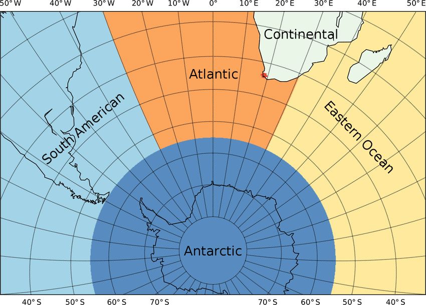
2 Methodology 2.3 Regionalisation
2.1 Observations The trajectories were categorised into six source regions de-
pending on their travel path (Fig. 3, Table 1). These cate-
This study is based on 10 years (2007–2016) of contin-
gories are as follows:
uous GEM measurements at Cape Point (CPT; 34◦ 210 S,
18◦ 290 E), South Africa. The CPT measurement site is part – Local. Air parcels which travelled less than 100 km ab-
of the GAW (Global Atmospheric Watch) baseline monitor- solute distance to CPT over the last 4 d are considered
ing observatories of the World Meteorological Organization to be local air masses.
(WMO). It is located at the southernmost tip of the Cape
Peninsula on top of the cliff at an altitude of 230 m (above – Continental. These are air parcels that spend more than
seal level). There are no major local Hg sources, and the 80 % of travel time over the African continent during
nearest city, Cape Town, is located 60 km to the north (see the last 4 d.
Atmos. Chem. Phys., 20, 10427–10439, 2020 https://doi.org/10.5194/acp-20-10427-2020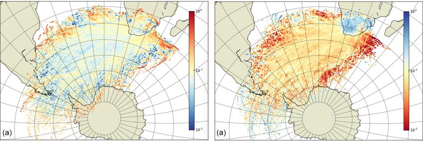
J. Bieser et al.: Atmospheric mercury in the Southern Hemisphere 10429
Figure 3. Depiction of the regionalisation used for this study: Lo-
cal (red), Continental (light green), Eastern Ocean (yellow), South
American (turquoise), Antarctic (blue), and Atlantic (orange).
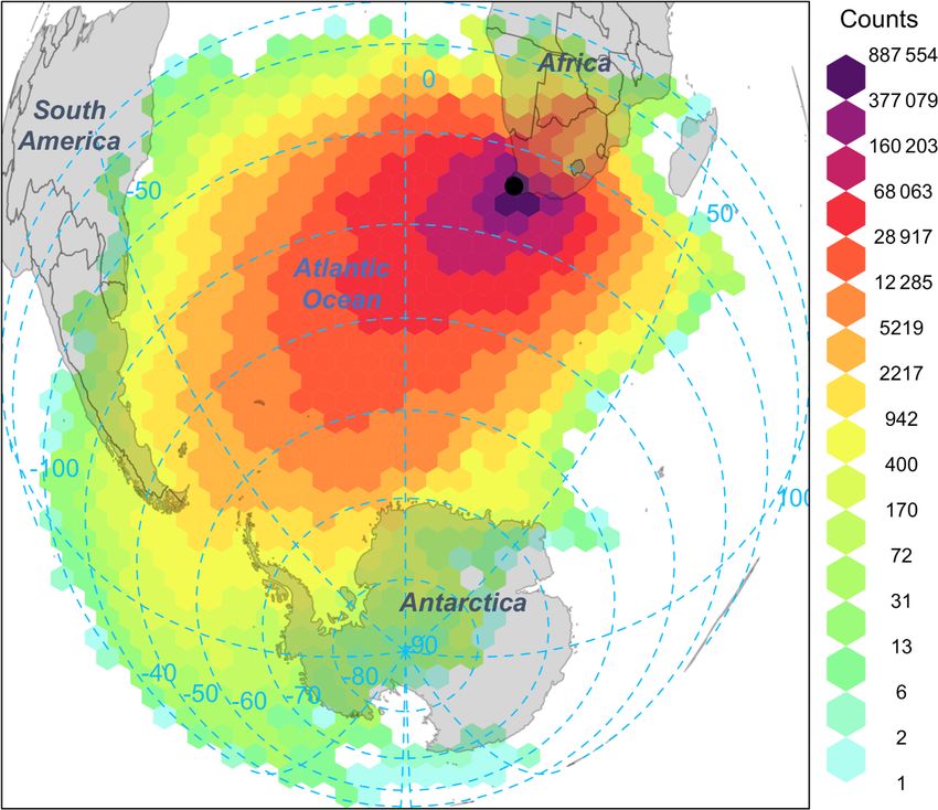
Figure 2. Origin of air masses influencing the Cape Point site (black
dot). Gridded back-trajectory frequencies using an orthogonal map
projection with hexagonal binning. The tiles represent the number CO, CO2 , CH4 , and O3 . 222 Rn is a radioactive gas of predom-
of incidences. The 2007–2016 hourly back trajectories were com- inantly terrestrial origin with a half-life of 3.8 d. Thus, high
puted using the HYSPLIT model (Stein et al., 2015), and the fig- 222 Rn concentrations mark air masses which recently passed
ure was made using the R package openair (Carslaw and Ropkins,
over the continent such as Continental and Local. Other ex-
2012).
amples are the distinction of long-range transport from South
America from Atlantic air masses. Here, we would also ex-
– Eastern Ocean These are air parcels which did not travel pect higher concentrations of other anthropogenic pollutants
over land and did not go west of 30◦ E within the last (e.g. CO2 , CH4 ).
4 d.
2.4 Identification of source/sink regions
– South American. These are air parcels which were west
of 30◦ W within the last 4 d. In order to evaluate source and sink regions we calculated the
10th and 90th percentile of GEM measurements for each sea-
– Antarctic. These are air parcels which were south of son – seasons being defined as 3-month intervals: DJF (sum-
55◦ S within the last 4 d. mer), MAM (autumn), JJA (winter), and SON (spring). This
seasonal filter proved to be necessary to remove the annual
– Atlantic. These are air parcels which do not fall within cycle in GEM concentrations driven (among others) by the
the other categories and spend more than 80 % of the seasonality of emissions, planetary boundary layer height,
time over the Atlantic Ocean. This category makes up and transport patterns. Furthermore, we filtered out mercury
the majority of all trajectories. depletion events, of unknown origin (Brunke et al., 2010),
which were defined as hourly average GEM concentrations
The categorisation of air parcels depends on the definition of less 0.25 ng m−3 .
of regions of origin and the travel time chosen for the algo- For the source/sink region analysis, we interpolated hourly
rithm. We calculated 5 d backward trajectories and experi- trajectory locations onto a polar stereographic grid centred
mented with different cutoff values to determine the source over the South Pole and calculated the total number of tra-
regions of the air masses (Table 1). For this study we chose jectories travelling through each grid cell over the 10-year
a cutoff time of 4 d to determine long-range transport from (2007–2016) period. We then performed the same proce-
Antarctica and South America. However, the choice of cutoff dure for the trajectories of the 10th and 90th percentile GEM
times of 3 or 5 d did not change the conclusions of our study. concentrations. By dividing these percentile maps by the to-
This decision is based on tests with different cutoff times and tal number of trajectories travelling through each grid cell,
on the fact that the uncertainty in the trajectories grows with we created maps indicating the regional prevalence of high
travel time (Engström and Magnusson, 2009). Moreover, air and low GEM concentrations. In the theoretical case of per-
parcels are often a mixture of different source regions (e.g. fectly homogeneous, evenly distributed sources and sinks,
Atlantic/Continental). As an additional test for the calculated each grid cell would have a value of 0.1 indicating that 10 %
categorisation we used secondary parameters such as 222 Rn, of all air parcels in each grid cell belong to the 10 % high-
https://doi.org/10.5194/acp-20-10427-2020 Atmos. Chem. Phys., 20, 10427–10439, 2020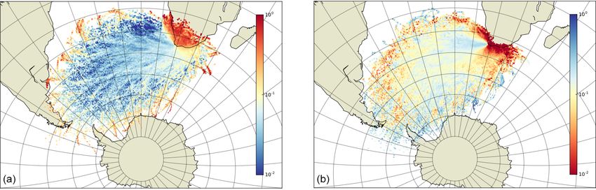
10430                                                           J. Bieser et al.: Atmospheric mercury in the Southern Hemisphere

Table 1. Impact of travel time cutoff on air parcels source region categorisation. Total and relative allocation of trajectories to each source
region depending on air parcel travel time.

                            Days     Antarctic    S. America     Continental    Eastern O.     Atlantic     Local
                            2            1778            150          14 580         5930      143478       1760
                                         (1 %)       (< 1 %)           (9 %)         (4 %)      (86 %)      (1 %)
                            3           11 800          3614          10 596         7842      132 876        926
                                         (7 %)          (2 %)          (6 %)         (5 %)      (79 %)      (1 %)
                            4           26 696         12 756          7928          7882      111 770        550
                                        (16 %)          (8 %)          (5 %)         (5 %)      (67 %)    (< 1 %)
                            5           39 710         22 960          5906          6876       91 666        370
                                        (24 %)         (14 %)          (4 %)         (4 %)      (55 %)    (< 1 %)

est/lowest GEM observations. Deviations from this uniform                 region, and the continent is the major sink region. We then
distribution are then interpreted as source/sink regions for              compare the regional patterns of GEM with other pollutants
high/low GEM concentrations. For example, a value of 0.2                  (Sect. 3.2 Comparison of regionalised data) and find that
indicates that twice as many high/low GEM concentrations                  GEM shows a distinct pattern compared to pollutants of ter-
originate from a given grid cell compared to a uniform dis-               restrial, anthropogenic and photochemical origin. In Sect. 3.3
tribution.                                                                Regional trends, we investigate distinct mercury trends for
   To better distinguish the 10th and 90th percentile plots,              each region. We find that air masses from long-range trans-
we chose opposite colour schemes for the 10th and 90th per-               port (South America, Antarctica) show no distinct trends,
centile plots. In the case of the 90th percentile plots, red              which indicates that they are representative of the SH back-
colour indicates source regions for high GEM concentra-                   ground. In Sect. 3.4 Regional abundance, we investigate what
tions (i.e. > 0.1), while blue colour indicates the absence of            impact changing atmospheric circulation may have on the
sources in this region (Fig. 4a). For the 10th percentile plots,          GEM trend observed at Cape Point and found it to be negli-
blue colour indicates sink regions for GEM concentrations                 gible. Instead we find that the annual average GEM concen-
(Fig. 4b), while red colour indicates the absence of sinks. It            trations depend on the regions with highest (Eastern Ocean)
is important to note that an absence of sources is not equal              and lowest (Continental) GEM concentrations in air masses.
to the presence of sinks and vice versa. Figure 4 gives an                Finally, in Sect. 3.5 Interannual variability, we try to explain
example of these plots for air masses attributed to the At-               the interannual variability in GEM concentrations observed
lantic category for 222 Rn measurements. This plot serves as              at Cape Point with changes in global emissions. We show
an evaluation of the regionalisation algorithm. It can be seen            that biomass burning and gold mining emissions can explain
that high 222 Rn concentrations are found only in air masses              years with exceptionally high (2014) or low (2009) GEM
that travelled over the continent (Fig. 4a). Similarly, Fig. 4b           concentrations.
depicts the fact that no measurements with low 222 Rn con-
centrations were found in air masses that travelled along the             3.1   Source and sink regions
coast line, indicating an impact of terrestrial sources. Finally,
this procedure is sensitive to the total number of trajectories           Figure 5 shows the 10th and 90th percentile maps for
travelling through a grid cell, which leads to low signal-to-             all GEM measurements over the whole period 2007–2016
noise ratios in the outskirts of the plot where only a few tra-           (Fig. 5). It can be seen that low GEM concentrations origi-
jectories originate at all. We used a cutoff value of 10 hits and         nate almost exclusively from air masses which travelled over
discarded all grid cells with fewer hits, but this still leads to         the continent (Fig. 5b). This result is in line with a clus-
a few nonsignificant hotspots at the outskirts of the domain              ter analysis performed by Venter et al. (2015), showing “air
(e.g. Fig. 4a in Antarctica).                                             masses that had passed over the very sparsely populated
                                                                          semiarid Karoo region, almost directly to the north of CPT
                                                                          GAW, were mostly associated with [. . . ] lower GEM values”.
3   Results and discussion                                                It is also consistent with the finding of Slemr et al. (2013) that
                                                                          southern Africa, based on GEM vs. 222 Rn correlations, is a
In this section we use backward trajectories of the 5th and               net sink region. The reason for this is probably a mixture of
95th percentile GEM concentrations observed at Cape Point                 near-zero emissions in the region and dry deposition onto the
to identify the major source and sink regions for mercury                 surface.
(Sect. 3.1 Source and sink regions). We find that the Eastern
Ocean with the warm Agulhas Current is the major source

Atmos. Chem. Phys., 20, 10427–10439, 2020                                                    https://doi.org/10.5194/acp-20-10427-2020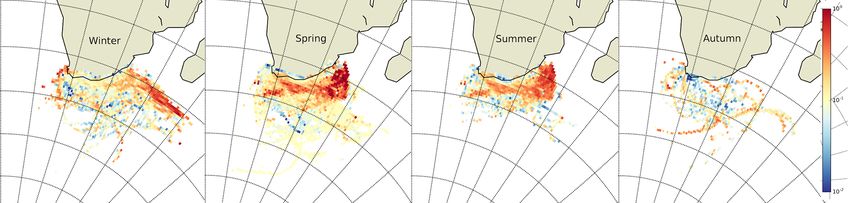
J. Bieser et al.: Atmospheric mercury in the Southern Hemisphere                                                                      10431

Figure 4. Distribution map for the (a) 90th percentile highest 222 Rn concentrations and the (b) 10th percentile lowest 222 Rn concentra-
tions measured at Cape Point. Values are the dimensionless prevalence of air parcels of a given concentration percentile ranging from 0 to 1.
This means that a homogeneous distribution of source and sink regions would lead to a plot with values of 0.1 everywhere. Deviations from
this value indicate source and sink regions. See also the description in Sect. 2.4.

Figure 5. Prevalence of (a) highest (90th percentile) and (b) lowest (10th percentile) GEM concentrations using all hourly trajectories over
10 years.

   Over the Atlantic Ocean, low GEM concentrations are                   certain source regions can be identified. These coincide with
in line with a uniform distribution with values mostly only              known major Hg emitters, mainly coal combustion for en-
slightly below the equilibrium value of 0.1. The exception               ergy production (Fig. 1). For air masses representing long-
are air masses that travelled over the ocean east of Cape                range transport (Atlantic, South American, Antarctic), fre-
Point where almost no low concentration GEM measure-                     quency values of the 90th percentile highest GEM concentra-
ments originated. Looking at the highest 90th percentile of              tions are mostly around 10 %, indicating no specific sources
GEM concentrations, air masses travelling over the ocean                 or sinks in these regions.
show a lower abundance with the exception of a patch east                   Looking at the 10th percentile of lowest GEM concentra-
of Cape Point (Fig. 5a).                                                 tions, regional and Continental air masses can be identified as
   The picture becomes clearer when plotting trajectories                the single most important sink region (Fig. 7a, b). There are
independently for each of the previously defined regions                 also some Continental areas with a high prevalence of low Hg
(Fig. 6). It can be seen that the Eastern Ocean sector is the            concentrations attributed to the Atlantic sector. These can be
predominant source region of air masses with elevated GEM                interpreted as air parcels with a mixed Continental/Atlantic
concentrations (Fig. 6e). In this region the Agulhas Current             travel path that have been attributed as Atlantic air masses
transports warm water from the Indian Ocean to the Atlantic              by the algorithm as they did not spend enough time over the
Ocean, and we identify this warm current as a major mercury              continent to be attributed to this sector. Finally, there are no
source in the region. For Continental air masses (Fig. 6b),

https://doi.org/10.5194/acp-20-10427-2020                                               Atmos. Chem. Phys., 20, 10427–10439, 2020
10432                                                      J. Bieser et al.: Atmospheric mercury in the Southern Hemisphere

Figure 6. 90th percentile highest GEM concentrations for air masses from six source regions. Red colour means source regions; blue means
an absence of emissions in that region.

air masses with low GEM concentrations originating from               Cape Point shown in Fig. 2 of the companion paper (Slemr
the Eastern Ocean sector (Fig. 7e).                                   et al., 2020). Temperature or primary production and a re-
   To further investigate the processes behind the observed           lated increase in evasion of GEM (with a large impact of re-
source and sink regions, we regard seasonal trajectory maps           emissions of legacy Hg) from the ocean are thus the likely
(Fig. 8). This analysis reveals that the high GEM concen-             reason for these observations.
trations associated with air masses from the Eastern Ocean
occur mainly during austral spring and summer. This is con-
sistent with the seasonal variation in GEM concentrations at

Atmos. Chem. Phys., 20, 10427–10439, 2020                                              https://doi.org/10.5194/acp-20-10427-2020
J. Bieser et al.: Atmospheric mercury in the Southern Hemisphere                                                                 10433

Figure 7. The 10th percentile lowest Hg concentrations for six source regions. Blue colours indicate sink regions, red colour absence of
sinks. Low values are almost exclusively linked to Continental and Local air masses.

3.2   Comparison of regionalised data                                    Table 2 shows the annual median GM concentrations. The
                                                                      highest annual median GEM concentrations were found for
Annual and monthly averages and medians for each source               Eastern Ocean in 6 of 10 years. The lowest annual GEM con-
region of 4 d backward trajectory were calculated for GEM,            centrations were almost always either of Local or Continental
CO2 , 222 Rn, CO, CH4 , and O3 . Here we compare the an-              origin. Annual median GEM concentrations for South Amer-
nual medians for all species and discuss the implications this        ican, Antarctic, and Atlantic lie close to each other and are in
comparison provides on regionalisation.                               the middle in varying order. Annual average GEM concen-
                                                                      trations behave similarly (not shown).

https://doi.org/10.5194/acp-20-10427-2020                                            Atmos. Chem. Phys., 20, 10427–10439, 2020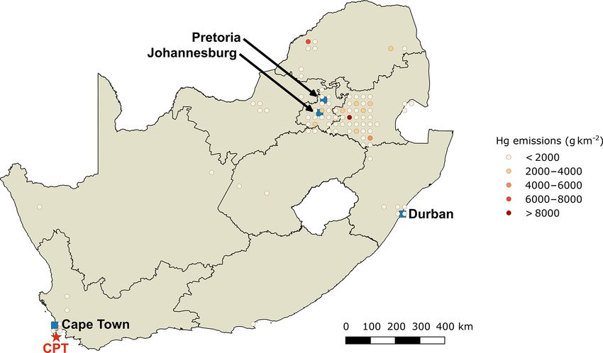
10434                                                       J. Bieser et al.: Atmospheric mercury in the Southern Hemisphere

Figure 8. Seasonal breakdown of 90th percentile highest Hg concentrations from the Eastern Ocean source region. Highest Hg concentrations
are mostly associated with austral spring and summer, which supports primary production as a potential source for oceanic Hg releases.

Table 2. Annual median GEM concentrations.

                   Year      Antarctic    South America     Continental      Eastern Ocean       Atlantic       Local
                                   Annual median GEM concentration (in ng m−3 ), number of measurements
                   2007    0.975, 2406       0.968, 1388     1.003, 412         1.046, 378    0.983, 6946   0.982, 39
                   2008    0.976, 1939        0.994, 811     0.992, 550         1.047, 453    1.002, 7903   0.883, 10
                   2009    0.910, 2457        0.904, 944     0.904, 950         0.933, 544    0.908, 9482   1.025, 27
                   2010    0.995, 2237       0.982, 1010     0.929, 918         1.036, 706   0.996, 10438   1.084, 18
                   2011    0.984, 1874        0.952, 941     0.978, 890        1.006, 1282    0.979, 8851   0.964, 69
                   2012    1.074, 2576       1.077, 1436     1.035, 453         1.063, 541   1.068, 10012   1.030, 62
                   2013    1.048, 2523       1.057, 1260     0.911, 555         1.069, 191    1.029, 8069   0.938, 48
                   2014    1.057, 2309        1.079, 947     1.045, 943         1.206, 929   1.098, 10791   1.090, 92
                   2015    1.009, 2330       1.009, 1020     0.992, 546         0.987, 482   0.998, 11486   1.017, 46
                   2015     1.030,2206        1.024, 990     0.986, 612         1.055, 740    1.015, 9935   0.934, 72

   Table 3 shows the annual median 222 Rn concentrations.              found either in Local or Continental, shows a pattern oppo-
The highest 222 Rn annual median concentrations were found             site to all the other species mentioned above. Its different pat-
for the regions Continental or Local, as expected for a ra-            tern clearly shows that its sources are predominantly oceanic
dioactive trace gas of almost exclusively terrestrial origin and       and the sinks terrestrial. The results reported above apply for
half-life of 3.8 d (Zahorowski et al., 2004). The lowest and           regionalisation using 4 d backward trajectories. Regionalisa-
second lowest 222 Rn concentrations were found in air masses           tion with 3 or 5 d backward trajectories provides similar re-
attributed to South American or Antarctic. Atlantic median             sults.
average concentrations are somewhat higher than Antarc-
tic and South American, but their interannual variation is             3.3     Regional trends
the smallest of all. Eastern Ocean median concentrations are
somewhat higher than the Atlantic ones, which is likely due            Table 4 shows the regionalised trends calculated from the
to proximity of African continent. The average concentra-              monthly median concentrations or mixing ratios. Region-
tions behave similarly.                                                alised trends for GEM, CO2 , 222 Rn, CO, CH4 , and O3 were
   The regionalised median annual mixing ratios of CO, CO2 ,           calculated from regional monthly averages and medians us-
CH4 , and O3 are shown in the Supplement. Annual medians               ing least-squares fit. Months with less than 10 measurements
of CO, CO2 , and CH4 , all of predominantly terrestrial ori-           were not considered. This restriction applies mostly to the
gin, behave similarly to those of 222 Rn. Ozone, although not          Local region, resulting in too few monthly values for trend
of terrestrial but of photochemical origin in NOx -rich envi-          calculation. The trends of 222 Rn and O3 are insignificant for
ronments, also fits this pattern because its mixing ratios are         all regions. The trend differences are tested for significance
highest in Local or Continental air masses where the high-             by comparison of averages (Kaiser and Gottschalk, 1972) us-
est NOx mixing ratios are expected. Annual averages behave             ing the slope and its uncertainty as an average and its stan-
similarly to annual medians.                                           dard deviation, respectively.
   In summary GEM, with highest concentrations in air                     The trends of 222 Rn and O3 are insignificant for all re-
masses attributed mostly to Eastern Ocean and the lowest one           gions. CO2 and CH4 upward trends are significant for all re-
                                                                       gions. The regional CO2 trends for the Antarctic and Atlantic

Atmos. Chem. Phys., 20, 10427–10439, 2020                                                https://doi.org/10.5194/acp-20-10427-2020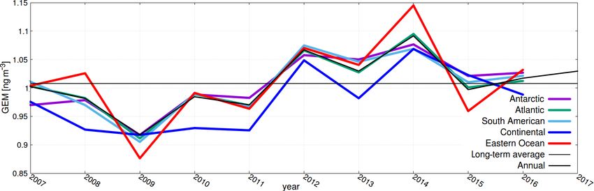
J. Bieser et al.: Atmospheric mercury in the Southern Hemisphere                                                               10435

Table 3. Annual median 222 Rn concentrations.

                    Year     Antarctic   South America      Continental     Eastern Ocean     Atlantic     Local
                                 Annual median 222 Rn concentration (in mBq m−3 ), number of measurements
                    2007    294, 2770           265, 1584     804, 432           685, 376    350, 8758    842, 38
                    2008    241, 1492            283, 604    2120, 502           345, 412    349, 6940
                    2009    230, 1982            275, 840    1623, 912           436, 548    345, 8306   1755, 26
                    2010    257, 1942            315, 780    2413, 784           449, 486    351, 9126   1326, 16
                    2011    208, 2546           288, 1086   2464, 1104          488, 1288   370, 10536   1612, 88
                    2012    184, 2658           231, 1510    1483, 548           413, 866   345, 10636   3273, 56
                    2013    252, 3104           174, 1650    2335, 630           489, 504   329, 10966   1709, 56
                    2014    249, 2296            255, 938    2195, 948           532, 968   337, 10928   1737, 74
                    2015    339, 2216           338, 1030    1786, 642           718, 564   348, 11510    803, 52
                    2015    244, 2346           209, 1296    2667, 626           530, 802   385, 10998   1656, 78

are comparable at 2.18–2.20 ppm yr−1 . The trends for Con-            masses differ significantly from the rest. On average, trans-
tinental and Eastern Ocean are also comparable, although              port from these two regions make up 10 % of the air masses
significantly higher, at 2.21–2.25 ppm yr−1 . The trend for           at Cape Point (Table 1). Their prevalence varies mostly only
South American is the smallest of all. The CH4 trends show            by 1 to 2 percentage points from year to year, with a peak
the same pattern with the trend for South American being              of 10 % Continental air masses in 2011. However, we found
the smallest, too. The trends for Antarctic and Atlantic are          that the prevalence of air masses from source and sink re-
comparable and somewhat higher. The trends for Continen-              gions is not the driver of the interannual variability in Hg
tal and Eastern Ocean are highest and comparable. The sim-            concentrations at Cape Point (e.g. even with twice as much
ilar pattern for CO2 and CH4 trends is consistent with terres-        as average air masses from the sink region, 2011 was not a
trial sources of these trace gases. The trend for CO is always        year with particularly low Hg concentrations) (Figs. 8, 9).
downward, although significant only for the South American            Because of this and based on the comparison with measure-
region when calculated both from monthly averages and me-             ments at Amsterdam Island (Slemr et al., 2020) we are confi-
dians.                                                                dent that mercury concentrations observed at Cape Point are
   Three source regions provide significant trends for GEM            representative for the Southern Hemisphere background. Ad-
when calculated both from monthly averages and medians.               ditionally, based on the presented work we are able to filter
The trends for Antarctic and South American air masses                out the source and sink regions from the dataset for further
are comparable and significantly higher than the trend for            analysis. Figure 10 depicts the whole GEM dataset with val-
the Atlantic region. This pattern is different from those of          ues from source and sink regions highlighted.
CO2 and CH4 , with smaller trends for South American and
higher ones for Atlantic and Antarctic. In summary, the pat-          3.5    Interannual variability
terns of GEM, CO2 , and CH4 trend differences provide ad-
ditional piece of evidence for an oceanic GEM source and              The trend in GEM concentrations observed at Cape Point
are consistent with the patterns of annual medians presented          and the fact that it seemingly changed from increasing to sta-
in Sect. 3.2. We note that the overall trend of GEM concen-           ble between 2006 and 2017 is still unexplained (Slemr et al.,
trations is close to that for the Atlantic region to which two-       2020). Having shown that the observations at Cape Point are
thirds of all GEM measurements are allocated.                         not dominated by regional processes, the question arises as
                                                                      to which large-scale processes modulate the signal on annual
3.4   Regional abundance                                              and decadal timescales.
                                                                         At this point, our null hypothesis is that mercury concen-
Air masses from long-range transport (Atlantic, Antarctic,            trations in the Southern Hemisphere were stable over the last
South American) make up 90 % of all air masses observed               decade, but processes on global and hemispheric scales su-
at Cape Point. Seasonally averaged observed concentrations            perimpose a (multi-)annual modulation on the signal. Based
from these regions show a high correlation with the aver-             on our analysis so far, we can exclude changes in climatology
ages of all observations at Cape Point, with R 2 values mostly        as the cause for the interannual variability. Thus, in our opin-
above 0.9 (Table 5). Only Antarctic air masses during austral         ion only global source processes remain as possible explana-
summer and autumn exhibit a lower correlation.                        tions for the observed anomaly. The identified processes are
   Air masses from the sectors Eastern Ocean and Conti-               marine emissions, emissions from biomass burning, and arti-
nental on the other hand show very low correlations with              sanal small-scale (ASGM) gold mining, which are the major
the averages observed at Cape Point indicating that these air         sources for mercury in the Southern Hemisphere.

https://doi.org/10.5194/acp-20-10427-2020                                             Atmos. Chem. Phys., 20, 10427–10439, 2020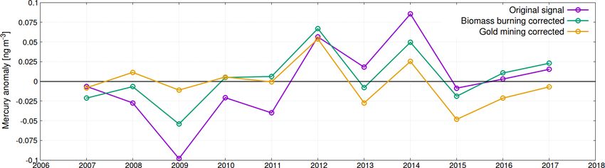
10436                                                      J. Bieser et al.: Atmospheric mercury in the Southern Hemisphere

Table 4. Trends of GEM, CO2 , CH4 , and CO calculated by least-squares fit from monthly averages (a) and medians (m). Months with less
than 10 measurements were not considered, which applies to most Local months. Trends of 222 Rn and O3 were not significant (ns) for all
regions.

                        Trace gas    Region             Slope                  N , significance   Unit
                        GEM          Antarctic          10.84 ± 2.63 (a)       112, > 99.9 %      pg m−3 yr−1
                                                        9.62 ± 2.69 (m)
                                     South American     10.16 ± 2.74 (a)       111, > 99.9 %
                                                        10.15 ± 2.80 (m)
                                     Continental        8.40 ± 4.25 (a)        91, ns
                                                        6.27 ± 4.02 (m)
                                     Eastern Ocean      5.20 ± 3.77 (a)        67, ns
                                                        6.33 ± 3.80 (m)
                                     Atlantic           8.64 ± 2.59 (a)        115, > 99 %
                                                        8.13 ± 2.54 (m)
                        CO2          Antarctic          2.186 ± 0.023 (a)      116, > 99.9 %      ppm yr−1
                                                        2.196 ± 0.022 (m)
                                     South American     2.171 ± 0.025 (a)      116, > 99.9 %
                                                        2.180 ± 0.022 (m)
                                     Continental        2.246 ± 0.048 (a)      90, > 99.9 %
                                                        2.226 ± 0.044 (m)
                                     Eastern Ocean      2.242 ± 0.049 (a)      73, > 99.9 %
                                                        2.210 ± 0.058 (m)
                                     Atlantic           2.182 ± 0.023 (a)      119, > 99.9 %
                                                        2.196 ± 0.019 (m)
                        CH4          Antarctic          6.320 ± 0.484 (a)      116, > 99.9 %      ppb yr−1
                                                        6.776 ± 0.391 (m)
                                     South American     5.789 ± 0.528 (a)      118, > 99.9 %
                                                        6.712 ± 0.395 (m)
                                     Continental        7.298 ± 0.708 (a)      95, > 99.9 %
                                                        6.732 ± 0.595 (m)
                                     Eastern Ocean      7.225 ± 0.695 (a)      76, > 99.9 %
                                                        7.230 ± 0.610 (m)
                                     Atlantic           6.670 ± 0.486 (a)      119, > 99.9 %
                                                        6.840 ± 0.388 (m)
                        CO           Antarctic          −1.166 ± 0.385 (a)     115, > 99 % (a)    ppb yr−1
                                                        −0.527 ± 0.260 (m)     ns (m)
                                     South American     −1.380 ± 0.397 (a)     117, > 99 % (a)
                                                        −0.731 ± 0.281 (m)     > 95 % (m)
                                     Continental        −1.027 ± 0.823 (a)     92, ns (a)
                                                        −1.055 ± 0.731 (m)     ns (m)
                                     Eastern Ocean      −0.010 ± 0.816 (a)     75, ns (a)
                                                        −0.133 ± 0.781 (m)     ns (m)
                                     Atlantic           −1.007 ± 0.364 (a)     119, > 95 % (a)
                                                        −0.506 ± 0.271 (m)     ns (m)

Atmos. Chem. Phys., 20, 10427–10439, 2020                                               https://doi.org/10.5194/acp-20-10427-2020
J. Bieser et al.: Atmospheric mercury in the Southern Hemisphere 10437
Figure 9. Annual average concentrations at Cape Point from 2007 to 2017 (black line) and regional averages (coloured lines). It can be seen
that the minimum in 2009 and the maximum in 2014 is present in all source regions.
Figure 10. Complete Cape Point dataset (grey) with observations originating from source (red) and sink (blue) regions superimposed. The
coloured x axis parallel indicates the long-term average (black: complete dataset; red: source region; blue: sink region).
Especially, the low mercury concentrations observed in 4 Conclusions
2009 and the high values observed in 2014 seem to be at least
partially a large-scale phenomenon. A screening of interna- Our goal was to improve the understanding of mercury cy-
tional observation networks also showed that Mace Head – cling in the Southern Hemisphere. For this, we combined
which is located in the Atlantic Ocean in the Northern Hemi- 10 years of GEM observations at Cape Point, South Africa,
sphere – also has the lowest annual average mercury con- with hourly backward trajectories calculated with the Hybrid
centrations in 2009 and the highest in 2014 (GMOS, 2020; Single-Particle Lagrangian Trajectory (HYSPLIT) model.
Weigelt et al., 2015). For the year 2009 the mercury emis- Our findings are as follows:
sion inventory of Streets et al. (2019) postulates a sudden
plummet in global gold mining activity. Comparing the an- 1. Overall the continent is a major sink region for mercury
nual anomaly from the 10-year average, gold mining activity despite significant point sources, mostly linked to coal
is correlated with observed GEM concentrations (R = 0.64). combustion.
Similarly, we found a correlation with biomass burning in the
Southern Hemisphere (mostly Africa) (R = 0.75) (Jiang et 2. Mercury emissions from the warm Agulhas Current to
al., 2017). We removed air masses from the identified source the south-east are a major source of elevated Hg con-
and sink regions from the dataset and used a regression anal- centration observed at Cape Point.
ysis to correct for changes in global gold mining and biomass
burning emissions (Fig. 11). The resulting signal becomes 3. Separating the ground-based observations into air
relatively flat, with only two peaks remaining in 2012 and parcels from different source regions showed that mer-
2014. cury behaves opposite to known pollutants of terrestrial
origin, implying the ocean as its major source.
https://doi.org/10.5194/acp-20-10427-2020 Atmos. Chem. Phys., 20, 10427–10439, 202010438 J. Bieser et al.: Atmospheric mercury in the Southern Hemisphere
Table 5. Correlation coefficient (R 2 ) of regional average concentrations with averages of all measurements at Cape Point. Values are based
on monthly averages (N = 30). Antarctic, Atlantic, and South American air masses exhibit a high correlation with the overall mean concen-
trations observed at Cape Point.
Annual Spring Summer Autumn Winter
(SON) (DJF) (MAM) (JJA)
Antarctic 0.89 0.95 0.75 0.72 0.96
South American 0.95 0.95 0.91 0.95 0.97
Continental 0.39 0.54 0.05 0.59 0.33
Eastern Ocean 0.81 0.77 0.58 0.14 0.84
Atlantic 0.98 0.97 0.90 0.94 0.99
Figure 11. Annual anomaly from 10-year average mercury concentrations. Original dataset at Cape Point (purple), corrected for biomass
burning emissions (green) (Jiang et al., 2017) and additionally corrected for gold mining emissions (orange) (Streets et al., 2019).
4. Mercury concentration in air masses from Antarctic, At- Data availability. Mercury observations at Cape Point are available
lantic, and South American origin were statistically al- via the GMOS data centre: http://sdi.iia.cnr.it/geoint/publicpage/
most indistinguishable. Thus, we interpret these obser- GMOS/gmos_monitor.zul (GMOS, 2020).
vations as a good representation of the southern hemi-
spheric background.
Supplement. The supplement related to this article is available on-
line at: https://doi.org/10.5194/acp-20-10427-2020-supplement.
5. We find that the trends in GEM concentrations postu-
lated in the past are probably an artefact of single years Author contributions. HA performed the HYSPLIT runs and inves-
with unusually high (2014) or low (2009) GEM concen- tigated emission and satellite data. LM is responsible for the obser-
trations (see accompanying paper: Slemr et al., 2020). vations at Cape Point. FS was responsible for the statistical evalu-
We have shown that these exceptional years could be ation. JB is the main author of the manuscript and was responsible
partly explained by changes in global emissions from for linking data from model and observation. All authors worked
collaboratively on the interpretation of the data.
biomass burning and gold mining, two major sources of
mercury in the Southern Hemisphere.
Competing interests. The authors declare that they have no conflict
of interest.
6. With the ocean being the main source of mercury in
the Southern Hemisphere it can be expected that an in-
creased air–sea flux due to larger concentration gradi- Acknowledgements. We want to thank NOAA for free access to the
ents will compensate reductions in global atmospheric HYSPLIT model. This publication forms part of the output of the
Biogeochemistry Research Infrastructure Platform (BIOGRIP) of
emissions due to the Minamata Convention. With this
the Department of Science and Innovation of South Africa as well
in mind we emphasise the need for more research on
as the newly formed South African Mercury Network (SAMNet).
marine mercury dynamics and air–sea exchange of mer-
cury.
Atmos. Chem. Phys., 20, 10427–10439, 2020 https://doi.org/10.5194/acp-20-10427-2020J. Bieser et al.: Atmospheric mercury in the Southern Hemisphere 10439
Lynwill Martin wishes to thank the CPT GAW team for providing R., and Joseph, D.: The NCEP/NCAR 40-year reanalysis project,
the data on which this paper is based. B. Am. Meteorol. Soc., 77, 437-470, 1996.
Martin, L. G., Labuschagne, C., Brunke, E.-G., Weigelt, A., Ebing-
haus, R., and Slemr, F.: Trend of atmospheric mercury con-
Special issue statement. This article is part of the special issue “Re- centrations at Cape Point for 1995–2004 and since 2007, At-
search results from the 14th International Conference on Mercury mos. Chem. Phys., 17, 2393–2399, https://doi.org/10.5194/acp-
as a Global Pollutant (ICMGP 2019), MercOx project, and iGOSP 17-2393-2017, 2017.
and iCUPE projects of ERA-PLANET in support of the Minamata NOAA Air Resources Laboratory (ARL): available at: http://ready.
Convention on Mercury (ACP/AMT inter-journal SI)”. It is not as- arl.noaa.gov/gdas1.php (last access: 1 March 2019), Tech. Rep.,
sociated with a conference. 2004.
Slemr, F., Brunke, E.-G., Labuschagne, C., and Ebinghaus, R.:
Total gaseous mercury concentrations at the Cape Point GAW
Financial support. This work has received funding under H2020- station and their seasonality, Geophys. Res. Lett., 35, L11807,
SC5-15-2015 ERA-NET-Cofund grant no. 689443 “Strengthening https://doi.org/10.1029/2008GL033741, 2008.
the European Research Area in the domain of Earth Observation”. Slemr, F., Brunke, E.-G., Whittlestone, S., Zahorowski, W., Ebing-
haus, R., Kock, H. H., and Labuschagne, C.: 222 Rn-calibrated
The article processing charges for this open-access publica- mercury fluxes from terrestrial surface of southern Africa, At-
tion were covered by a Research Centre of the Helmholtz mos. Chem. Phys., 13, 6421–6428, https://doi.org/10.5194/acp-
Association. 13-6421-2013, 2013.
Slemr, F., Weigelt, A., Ebinghaus, R., Bieser, J., Brenninkmeijer,
C. A. M., Rauthe-Schöch, A., Hermann, M., Martinsson, B.
G., van Velthoven, P., Bönisch, H., Neumaier, M., Zahn, A.,
Review statement. This paper was edited by Andreas Hofzumahaus
and Ziereis, H.: Mercury distribution in the upper troposphere
and reviewed by two anonymous referees.
and lowermost stratosphere according to measurements by
the IAGOS-CARIBIC observatory: 2014–2016, Atmos. Chem.
Phys., 18, 12329–12343, https://doi.org/10.5194/acp-18-12329-
References 2018, 2018.
Slemr, F., Martin, L., Labuschagne, C., Mkololo, T., Angot, H., Ma-
Amos, H. M., Jacob, D. J., Streets, D. G., and Sunderland, E. gand, O., Dommergue, A., Garat, P., Ramonet, M., and Bieser,
M.: Legacy impacts of all-time anthropogenic emissions on the J.: Atmospheric mercury in the Southern Hemisphere – Part
global mercury cycle, Global Biogeochem. Cy., 27, 410–421, 1: Trend and inter-annual variations in atmospheric mercury
https://doi.org/10.1002/gbc.20040, 2013. at Cape Point, South Africa, in 2007–2017, and on Amster-
Baker, P. G. L., Brunke, E.-G., Slemr, F., and Crouch, A.: Atmo- dam Island in 2012–2017, Atmos. Chem. Phys., 20, 7683–7692,
spheric mercury measurements at Cape Point, South Africa, At- https://doi.org/10.5194/acp-20-7683-2020, 2020.
mos. Envron. 36, 2459–2465, 2002. Stein, A. F., Draxler, R. R., Rolph, G. D., Stunder, B. J. B., Cohen,
Brunke, E.-G., Labuschagne, C., Ebinghaus, R., Kock, H. H., and M. D., and Ngan, F.: NOAA’s HYSPLIT Atmospheric Transport
Slemr, F.: Gaseous elemental mercury depletion events observed and Dispersion Modeling System, B. Am. Meteorol. Soc., 96,
at Cape Point during 2007–2008, Atmos. Chem. Phys., 10, 1121– 2059–2077, 2015.
1131, https://doi.org/10.5194/acp-10-1121-2010, 2010. Streets, D. G., Horowitz, H. M., Lu, Z., Levin, L., Thackray, C.
Carslaw, D. C. and Ropkins, K.: openair – An R package for air P., and Sunderland, E. M.: Global and regional trends in mercury
quality analysis, Environ. Modell. Softw., 27–28, 52–61, 2012. emissions and concentrations, 2010–2015, Atmos. Environ., 201,
Engström, A. and Magnusson, L.: Estimating trajectory uncertain- 417–427, 2019.
ties due to flow dependent errors in the atmospheric analysis, UNEP: The Minamata Convention on Mercury, available at:
Atmos. Chem. Phys., 9, 8857–8867, https://doi.org/10.5194/acp- http://www.mercuryconvention.org/Countries/tabid/3428/
9-8857-2009, 2009. language/en-US/Default.aspx (last access: 17 June 2019), 2013.
GMOS: Global Mercury Observation System, CNR-Institute Venter, A. D., Beukes, J. P., van Zyl, P. G., Brunke, E.-G.,
of Atmospheric Pollution Research, Rome, Italy, available Labuschagne, C., Slemr, F., Ebinghaus, R., and Kock, H.: Sta-
at: http://sdi.iia.cnr.it/geoint/publicpage/GMOS/gmos_monitor. tistical exploration of gaseous elemental mercury (GEM) mea-
zu, last access: 19 August 2020. sured at Cape Point from 2007 to 2011, Atmos. Chem. Phys.,
Jiang, Z., Worden, J. R., Worden, H., Deeter, M., Jones, D. B. 15, 10271–10280, https://doi.org/10.5194/acp-15-10271-2015,
A., Arellano, A. F., and Henze, D. K.: A 15-year record of 2015.
CO emissions constrained by MOPITT CO observations, At- Weigelt, A., Ebinghaus, R., Manning, A. J., Derwent, R.G., Sim-
mos. Chem. Phys., 17, 4565–4583, https://doi.org/10.5194/acp- monds, P., Spain, T. G., Jennings, S. G., and Slemr, F.: Analysis
17-4565-2017, 2017. and interpretation of 18 years of mercury observations since 1996
Kaiser, R. and Gottschalk, G.: Elementare Tests zur Beurteilung von at Mace Head, Ireland, Atmos. Environ., 100, 85–93, 2015.
Messdaten, Bibliographisches Institut, Mannheim, 1972. Zahorowski, W., Chambers, S. D., and Henderson-Sellers, A.:
Kalnay, E., Kanamitsu, M., Kistler, R., Collins, W., Deaven, D., Ground-based radon-222 observations and their application to at-
Gandin, L., Iredell, M., Saha, S., White, G., Woollen, J., Zhu, Y., mospheric studies, J. Environ. Radioactiv., 76, 3–33, 2004.
Chelliah, M., Ebisuzaki, W., Higgins, W., Janowiak, J., Mo, K.
C., Ropelewski, C., Wang, J., Leetmaa, A., Reynolds, R., Jenne,
https://doi.org/10.5194/acp-20-10427-2020 Atmos. Chem. Phys., 20, 10427–10439, 2020You can also read