Report on the Geant4 simulations performed for the "Realisation of the Bq" project - Gabriel Suliman
←
→
Page content transcription
If your browser does not render page correctly, please read the page content below
Report on the Geant4 simulations
performed for the "Realisation of the
Bq" project

                      Gabriel Suliman

                      2013

                                        Report EUR 25676 EN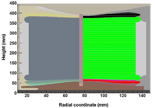
European Commission
Joint Research Centre
Institute for Reference Materials and Measurements

Contact information
Uwe Wätjen
Address: Joint Research Centre, Retieseweg 111, B-2440 Geel, Belgium
E-mail: uwe.waetjen@ec.europa.eu
Tel.: +32 14 571 882
Fax: +32 14 584 273

http://irmm.jrc.ec.europa.eu/
http://www.jrc.ec.europa.eu/

Legal Notice
Neither the European Commission nor any person acting on behalf of the Commission
is responsible for the use which might be made of this publication.

Europe Direct is a service to help you find answers to your questions about the European Union
Freephone number (*): 00 800 6 7 8 9 10 11
(*) Certain mobile telephone operators do not allow access to 00 800 numbers or these calls may be billed.

A great deal of additional information on the European Union is available on the Internet.
It can be accessed through the Europa server http://europa.eu/.

JRC78190

EUR 25676 EN

ISBN 978-92-79-28074-0

ISSN 1831-9424

doi:10.2787/70585

Luxembourg: Publications Office of the European Union, 2013

© European Union, 2013

Reproduction is authorised provided the source is acknowledged.

Printed in Belgium
1. Introduction ........................................................................................................................ 2
2. The simulation program ..................................................................................................... 3
   2.1 The physical processes ................................................................................................. 4
   2.2 The geometry................................................................................................................ 4
   2.3 The particle source ....................................................................................................... 5
   2.4 The analysis.................................................................................................................. 5
3. Simulation results............................................................................................................... 7
   3.1 Comparison with previous simulations ........................................................................ 7
   3.2 Studies concerning the thickness of the inner wall of the ionisation chamber ............ 9
   3.3 Study of the influence of the material composition for the inner wall of the IC ....... 13
   3.4 Simulations supporting the new prototype................................................................. 15
References ............................................................................................................................ 20
Additional information......................................................................................................... 21
   Appendix 1: The configuration file.................................................................................. 21
   Appendix 2: Particle source file ....................................................................................... 22
   Appendix 3: Analysis file................................................................................................. 23
   Appendix 4: Geometry file............................................................................................... 24
   Appendix 5: Precision of the simulation .......................................................................... 28
   Appendix 6: Charge collection......................................................................................... 29

                                                                                                                                        1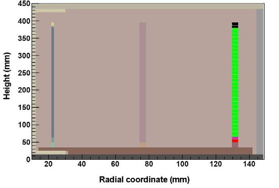
1. Introduction

        The main objective of the "Realisation of the Bq at basic level" project is to
develop a "fully" reproducible 4π ionisation chamber. For this purpose, all the
dimensional and operational parameters of the chamber have to be described in the
construction specifications to ensure that any chamber build accordingly will display an
almost identical response function. The acceptable variation of the response between
two such "identical" ionisation chambers should be bellow 0.2% for a broad energy
range (20 keV‐ 2 MeV).
        Monte Carlo simulations have become an integral part of developing new
radiation detectors and the work on the ionisation chamber that is being built as part of
this project makes no exception. Until now, Monte Carlo simulations were performed at
IRMM using EGS4 [1] and MCNP5 [2] and at LNHB using Penelope [3]. Some of these
simulations were used to define the parameters of a prototype ionisation chamber,
while others dealt with other aspects of the operation of the chamber such as the effect
of the ampoules holding the source, or the positioning of the ampoule. In 2010 the work
started on designing a new prototype. At the same time, a new simulation program for
the project was started, using the Geant4 [4] framework.
        This technical document will present the details of the simulations as they were
performed using the Geant4 [4] framework, focusing on the last version of the
simulation code. This document, together with the source code and the documentation
included in the source code should provide enough information for anyone to reproduce
the results and expand the simulations.

Why Geant4?
       Of the existing Monte‐Carlo simulation packages, Geant4 is probably the most
powerful, and at the same time the most complex. The way the package is built allows
much better access to all the stages of the simulation, but at the cost of a slight increase
in complexity; a bonus point is that the ROOT framework can be used to analyse the
results of the simulations.
       Another reason is that the geometry description is more free and closer to a
natural description of the object, allowing arbitrary positioning of the geometry
components (for example in scenarios where the influence of the tilting of a structural
element is studied). Materials of any composition and complexity can be used, and
additional properties of the detector, for example charge collection effects, can be
included.

Purpose of the simulation program
       The main goal of the simulation program is to assist in the decision making
process for the new prototype of the ionisation chamber that is currently in the design
phase. Because of the reproducibility emphasis of the project the simulation program
must be appropriate not only to assess the performance of the Ionisation Chamber but
also to study how the performance is influenced by small deviations from the nominal
values of the components.

                                                                                          2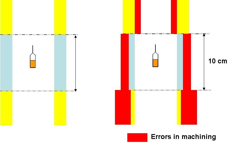
2. The simulation program

       The philosophy of the Geant4 framework requires the user to implement four
areas of the simulation (or, in C++ terms, to provide implementations for four virtual
classes): the physical processes (which allows the study of how important different
interaction mechanism are), the particle source, the geometry of the detector (the
ionisation chamber) and the analysis that should be performed on the results of the
simulation. Once this information is provided, the Geant4 framework will generate
particles according to the implementation of the source provided by the user, will
transport and make the particles interact with the detector according to the physics list
and geometry and will, on an event by event basis, analyse the results.

        In a typical program following the Geant4 patterns, all of these would be
hardcoded in the source code. For example, all of the details of the geometry would be
described in C++ language (using the classes provided by Geant4) and any modification
to the geometry would require editing and recompiling of the source code. We have
found that this approach is lacking for the scope of our project because of the type of
studies that we were interested to perform. For example, studying the sensitivity of the
response to the thickness of the inner tube of the ionisation chamber, where the result
for five thicknesses are compared would require, on one hand, recompiling the code, but
also modifying the description of the detector in the source code five times, at all the
places where the geometry is affected. It is clear that this leads to problems in detecting
any error that might occur in the process, and also makes repeating a simulation
somewhat difficult. Saving the compiled executable file is only a partial solution, as the
changes between compiled executables cannot be identified. To overcome this issues the
implementation of the required classes was performed in a generic way, with all the
numerical parameters read from external files.

        During the course of the project it became obvious that the study of the way the
collection of charges takes place in the IC is of the highest importance. This is
traditionally left out of the Monte‐Carlo simulations (whose sole purpose is to determine
how and where the energy is deposited inside the detector). As a result, the analysis part
of the simulation was extended to include the charge collection.

Technical details
       The programming language used by the simulation (and Geant4) is C++. The
analysis takes advantage of the excellent data analysis abilities of the ROOT framework
[5] (C++). Extra care was taken so that the computer code itself is as well documented as
possible (doxygen [6] The management of the versions of the code was performed using
CVS [7].

 The hierarchy of the external files is:
    ‐ ICsetup.inp: the master configuration file, contains the name of the files where all
the other information will be read. This is the only filename coded in the program, so a
file with this name must exist in the run directory (see Appendix 1 for an example of
input file with description of the fields)
    ‐ files describing the simulation scenario being investigated

                                                                                         3
‐ file with the description of the particle source
‐ geometry description file
‐ analysis file
‐ file with the charge collection map
‐ files with description of real sources
2.1 The physical processes
The default physics processes used by Geant4 have been proven inadequate at
the low energies of interest for the project (Geant4 was developed at CERN to be used in
high‐energy physics experiments). The simulation community became aware of this
issue soon after the launch of Geant4 and a few groups undertook the initiative to
develop interaction packages that can be used at low energy. One of these approaches
rewrote the physical processes implementation from Penelope [8] and made it available
in Geant4.
Our choice of low energy package is the Penelope implementation, and at all
times during the simulations all the processes were kept active.
The cut‐offs are also declared during this part of the simulation. In Geant4 the
range cut‐off represents the accuracy of the stopping position. It does not mean that the
track is killed at that energy. The value of the cut‐off is defined in the "ICsetup.inp" file,
and, in most cases, a value of 10 μm was used.
2.2 The geometry
The geometry of the detector constitutes one of the most important parts of the
simulation code. Geant4 provides the user with a whole array of building blocks that can
be used to generate geometries of any complexity. In principle these building blocks are
used as part of the C++ code, and the geometries are "hardcoded" in the simulation.
Compared to the detectors at CERN that were the aim of the Geant4 simulation
package, the ionisation chamber is a relatively simple detector. Another factor that was
taken into account is that for the current project we are not interested so much on the
response of the detector as we are on its sensibility to variations of the dimensions of
the components of the ionisation chamber. That is to say that the goal of the simulation
is not to assess the response of the chamber but to estimate the tolerances on the
components.
As a result, we have decided to not hardcode the geometry in the C++ code but to
implement another layer of geometry description that allows changes of the geometry
without recompiling the code. This approach has also the advantage that once the
source code is compiled, simulations can be run without knowledge of the inner
workings of the program, simply by changing the parameters in the input file.
The geometry is described in terms of a restricted set of building blocks, which
are better suited to describe the geometry of the ionisation chamber than the (more
general) Geant4 building blocks. This simplification arises from the cylindrical geometry
of most of the components of the ionisation chamber.
The ionisation chamber is described (following the Geant4 pattern) as a
hierarchical structure of objects, where any component must be part of another one.
Each of the components of the ionisation chamber is described by a single line in the
input file.
4An example of geometry input file and more details about how the geometry is
described are presented in Appendix 4.
As a side note, the Geant4 framework allows arbitrary complexity geometries to
be imported directly from CAD programs. We have found that the geometry of the
ionisation chamber is too simple to justify the overhead of using this feature.
2.3 The particle source
The response of the IC to single energy particles forms the basis of the studies
that are performed using the Monte‐Carlo method. This is useful in most circumstances
but it does not translate easily in methods to test whether a component of the ionisation
chamber is out of specifications. To address this issue, the particle source for the
simulation was written so it allows not only single energy particles, but also continuous
distributions (for β+ and β‐ decays) and full radionuclides, with all possible combinations
of emitted particles and emission probabilities.
Each of the radionuclides are described in text files that are distributed at the
same time with the source code. The list of radionuclides can be extended by supplying
the appropriate isotope description file.
An example of a source input file can be found in Appendix 2.
2.4 The analysis
The analysis is that part of the program where the energies deposited at each
interaction in a sensitive component are put together to calculate the response of the
ionisation chamber. In our simulation we have implemented two types of analysis. The
first one deals with the energy deposited in each of the components. The second one
uses a model of the field distribution inside the chamber to analyse only the interactions
in the sensitive area of the gas, and which are collected by the electrodes.
In both cases the mean deposited (or collected) energy is calculated following the
analysis described in the MCNP manual [2] (and described in Appendix 5) .
Charge collection
When dealing with detectors, the problem of charge collection is usually left aside
because in most cases all the energy deposited in the detector is collected and measured.
This is not the case in an ionisation chamber, where guard rings divide the sensitive gas
volume defining parts that will not yield any signal in the collecting electrodes, no
matter the amount of energy deposited. This effect is expected to be important because
the plans for the next prototype foresee a number of such dead volumes.
In the case of an ionisation chamber we can safely assume that any charge
generated in the collection area of the gas will be collected. This is not entirely true, but
the high intensity of the field due to the high voltage will decrease the influence of the
charge losses through recombination .Also, as we are interested in the variation of the
response between two identical chambers, we are assuming that the variation in loses
between such two chambers is negligible for the scope of the project.
The charge collection was included in the simulation as an additional step of the
analysis of the interaction in the materials. For each interaction that takes place in the
gas we are interested to find out where the charges are collected: the electrodes, the
5guard rings or the other structural elements. For that, a finite‐element method (FEM)
software (ELMER [9]) was used to calculate the field distribution in the chamber.
Taking advantage of the cylindrical symmetry of the ionisation chamber, the FEM
method is used in a two‐dimensional space, made by half of the cross‐section through
the IC, and the tracking of particles in this field is performed in Geant4.
Unless otherwise specified, in the following section, the response of the chamber
refers to the energy deposited in the "collectable" region of the gas, and not to the
energy deposited in the total gas volume.
More details about the charge collection procedure can be found in Appendix 6.
63. Simulation results
In this chapter some of the results of the simulations will be presented. The goal of the
simulations is to study the design of the new prototype, but in some cases the existing
prototype (the RWD chamber) was used.
Without going in the details of the differences between the two designs, the following
pictures present the schematic drawings of the two chambers, as they were used in the
simulations.
Figure 1: The RWD design Figure 2: The IC2010 design
3.1 Comparison with previous simulations
In this section we will present two comparisons between results obtained with the
simulation code developed using Geant4 and results obtained previously in the project
in order to verify the correctness of the code implementation.
3.1.1 Response to mono-energetic photons
Previously [10], the results of Monte‐Carlo simulations using MCNP5 and
Penelope were compared for the case of a simple geometry and a good agreement was
found between them. While a full comparison between our code in identical conditions
might seem justified, it would only replicate some of the in‐depth studies comparing the
available Monte‐Carlo codes [11]. As a result we have opted for comparing the results of
the real geometry of the prototype obtained with Geant4 with those of a similar (more
simple) geometry used in the previous comparison (where only the vertical components
of the prototype were included).
In addition to the geometry difference, for the Geant4 simulation we have used
two type of sources:
point‐like mono‐energetic gamma source (similar to that used in the previous
comparison)
a more realistic mono‐energetic source: the described source consists of mono‐
energetic emitters dissolved in water, contained in an glass ampoule (uniform
distribution of source emitters from a "water" cylinder, surrounded by the ampoule)
7The results of the comparison can be seen in figure 3. It can be seen that the
results are in agreement at low energy where the energy deposition is limited to the
volume in the center of the chamber (far away from the regions of difference between
the geometries) and at high energies, where the deposited energy depends the least on
the geometrical details of the chamber and more on the total mass of gas present in the
chamber.
Figure 3: comparison between Geant4 and MCNP/Penelope simulations
10
Deposited energy in gas (keV/Bq)
1
Geant4
Penelope
MCNP
Geant4 no ampoule
0.1
0.01 0.1 1
Energy (MeV)
Another aspect that becomes clear from these simulations is the huge effect that the
ampoule and the water solution that contains the source have on the response of the
chamber.
3.1.2 Tolerance on the thickness of the inner wall if Al is used
The tolerances on machining the inner wall of the ionisation chamber are among
the critical parameters in achieving the required 0.2% reproducibility because of the
high attenuation rate at low gamma energy. This is why these tolerances were
previously studied to a great extent [10], using both an analytical model and MCNP5.
For both this reasons, performing the same study using the Geant4 code is one of the
most important tests that a successful simulation program needs to pass.
Simulations were performed for the prototype chamber using a point‐like mono‐
energetic gamma source. The only parameter that was modified between the simulation
runs was the thickness of the inner wall. Seven simulation runs were performed,
starting with the nominal thickness of 2mm and using both higher and lower
thicknesses with a deviation of a few µm from the nominal value (±3 µm, ±5µm, ± 10 µm
and 30µm). The study used only low energy photons ( 20 keV, 30 keV and 50 keV)
because the effect on the response is decreasing with increasing energy.
Figures 4 show the results of the simulation. The figure on the left side shows the
full results, while the one on the right shows a detail concentrating on the results around
the nominal value. In the second figure we represented with dashed line the 0.2%
accepted deviation on the response that is deemed acceptable for the project. It can be
seen that the curve corresponding to 20 keV intersects this curve very close to the
nominal values, in agreement with the 2μm tolerance at 20 keV obtained in the previous
8studies. It can also be seen that the tolerance increases rapidly with increasing energy,
so that a tolerance of roughly 12µm is needed to fulfil the goal of the project at 50 keV.
Figure 4: deviation from the ideal response in the presence of deviations of inner wall thickness
1.03 1.008
1.007
20 keV 20 keV
1.02 1.006
30 keV 30 keV
1.005
50 keV 50 keV
Deviation from nom inal value
D eviation from nominal value
1.01 1.004
1.003
1.00 1.002
1.001
0.99 1.000
0.999
0.98
0.998
0.997
0.97
0.996
0.995
0.96
0.994
0.95 0.993
0.992
-10 0 10 20 30 -10 0 10 20 30
Dev iation on the thic kness of the Inner Wall (m ) Deviation on the thic kness of the Inner Wall (m)
3.2 Studies concerning the thickness of the inner wall of the ionisation
chamber
The thickness of the inner wall of the ionisation chamber was identified as one of the
bottle necks in successfully fulfilling the goals of the project. This is due to the fact that
achieving 2 μm tolerance on what is basically a tube 40 cm long, inner diameter of 3 cm
and a wall thickness of 2 mm is beyond any existing machining possibility.
To address this issue we have investigated a number of possibilities, using both
simulations and enquiring about manufacturing procedures. This section focuses on the
results of the simulations for these scenarios.
3.2.1 Tolerance on the thickness of the inner wall if other materials can be used
The first scenario that was investigated is the possibility to have the inner wall of
the ionisation chamber made of a different material instead of Aluminium. It is obvious
that the only way to ease the tolerances on the thickness is to use a material with lower
absorption than Aluminium, which can only be achieved by using a material (or alloy)
with a lower atomic number. Another critical constraint is that the ionisation chamber
needs to be pressurised to 2 MPa, so the material should be mechanically strong. After a
search of the materials available on the market we found two other materials that seem
fit for the purpose: AZM [12], a Mg‐Al alloy used in aeronautics and a Be‐Al alloy (S200F
[13]) that can be used for structural components.
Simulations to establish the required machining tolerances were performed for
all three possibilities: Aluminium, AZM and S200F.
The figures bellow show the variation of the response, as a function of the
deviation from the nominal values of the thickness of the inner wall for the three
materials. The horizontal dotted lines denote the acceptable limits for the project
(0.2%).
9Figure 5: influence of the deviations from design values of the the inner wall thickness for different
materials
20 keV
1 .0 0 8 A l2 0 2 4 30 keV
50 keV
1 .0 0 4
1 .0 0 0
0 .9 9 6
Deviation from nominal value
0 .9 9 2
1 .0 0 8 A Z M ( M g a llo y )
1 .0 0 4
1 .0 0 0
0 .9 9 6
0 .9 9 2
1 .0 0 8
S 2 0 0 F ( B e a llo y )
1 .0 0 4
1 .0 0 0
0 .9 9 6
0 .9 9 2
-1 0 0 10 20 30
D e v ia t io n o n th e t h ic k n e s s o f th e In n e r W a ll (m m )
It can be seen that compared to Al, the use of AZM is a much better solution (5 μm
tolerance), while the use of Be would remove any constraint on the tolerance of the
inner tube, Practically, if Be is used, the response is independent of the thickness of the
tube for the interval we have studied. (Employing the analytical model, the required
tolerance for a Be inner wall is of the order or 100 µm).
While this approach seems to solve the problem of the tolerance of the inner wall
there are still a number of concerns of which we will only mention two: the very high
price of the Be‐Al tube and the toxicity of Be.
3.2.2 The use of compensation Al foils
Another work‐around envisaged for the problem of having technically
unachievable tolerances for the inner tube thickness is to employ thin aluminium foils,
which would surround the ampoule or the holder to compensate for the thickness
differences between chambers. The purpose of the simulation was to see whether such
an approach would give the required results.
Three scenarios were studied, each for four energies (20 keV, 30 keV, 50 keV and
70 keV) . In each of the scenarios, the response of the chamber for a thinner inner wall
was compared with the nominal response and with the the response obtained by adding
a thin Al foil to compensate the difference. The three scenarios assumed a difference
between the real thickness and the nominal thickness of 30 μm, 50 μm and 100 μm. The
three deviation values that were used in this case correspond to estimated realistic
tolerances for the inner wall of the prototype.
10Figure 6: compensation of the inner wall deviations if compensation foils are used
1 .2 0
100 m 50 m 30 m
1 .1 5 2 0 k e V
Deviation from nominal value
3 0 k e V
5 0 k e V
7 0 k e V
1 .1 0
1 .0 5
1 .0 0
al r ed al r ed al r ed
in ne at in ne at in ne at
m in ns m in ns m in ns
No Th pe No Th pe No Th pe
m m m
Co Co Co
In n e r w a ll th ic k n e s s
As it can be seen from the figure above, compensating the thickness of the inner
wall with thin Aluminium foils is a viable procedure, and that a properly measured foil
can compensate for the deviations in machining the inner wall. Of course, this approach
has a few drawbacks in itself: while much higher machining precision can be achieved in
machining the compensation foil, it is almost impossible at this time to measure how
thick it should be, because measuring the thickness of the inner tube is a very
complicated issue. Also, this approach will add to the complexity of the operation of the
ionisation chamber because another component (the compensation foil) needs to be
taken care of while manipulating the source. More issues can be foreseen when the
replacement of the foil has to be performed.
3.2.3 Inner tube made of three sections machined to different tolerances/accuracies
The purpose of the simulation presented in this section is to investigate whether
the inner tube can be made of three shorter sections, each of them easier to machine,
which are then welded together.
This idea has its basis in the fact that the two dimensional maps show that most
of the response comes from photons that went through the inner tube in a rather
narrow region around the position of the ampoule. Another starting point for the
simulation was given by the fact that the much better tolerances can be achieved on
machining a 10 cm long tube, which is then welded to other pieces to form the inner
tube of the ionisation chamber.
For the simulation (figure 7), the inner tube was divided in three segments, the
middle one, centred on the source position, being 10 cm long. The goal of the simulation
was to study to what extent achieving a very good machining accuracy for the central
piece can compensate for having the other two pieces machined to very bad accuracy. Of
course, the number of possibilities that can be studied is enormous (with both the outer
pieces being thicker or thinner than the nominal value), so only two scenarios were
chosen: the outer sections have the same thickness, which is higher or lower from the
nominal value by 100 µm. For the central piece five thicknesses were considered: the
nominal value, thicker by 10 or 20 μm or thinner by 10 or 20 μm.
11Figure 7: possible scenarios for the tolerances if the inner tube is made of three sections
The results of the simulation are presented in the figure bellow, where the
normalisation is done to a inner tube at nominal values. The dashed lines represent the
acceptable variation in response that has to be achieved in the project.
Figure 8: deviation from the ideal response in the presence of deviations of central piece thickness
O u t e r s e c t io n s O u te r s e c tio n s
th in n e r b y 1 0 0 m t h ic k e r b y 1 0 0 m
1 .0 4 1 .0 4
20 keV
30 keV
Deviation from nominal value
50 keV
1 .0 2 1 .0 2
70 keV
1 .0 0 1 .0 0
0 .9 8 0 .9 8
0 .9 6 0 .9 6
-2 0 -1 0 0 10 20 -2 0 -1 0 0 10 20
D e v ia tio n f r o m n o m in a l v a lu e o f t h e c e n t r a l p ie c e
It can be seen that the predominant factor in the deviation from the response of the
"ideal" inner wall can be traced to the variation of the central section. Also, it appears
that the tolerance that needs to be achieved for this case is of a few micrometers,
basically the same that needs to be achieved by the whole inner wall, in the hypothesis
that it is made of a single piece.
While the machining complexity is reduced, in that only the central piece needs to be
machined with a very good tolerance, this approach adds complexity in the required
technologies to weld together the three tubes so that they are both leak‐tight and
structurally sound. Additional issues might arise from the alignment of the three
components during/after the welding procedure.
123.3 Study of the influence of the material composition for the inner wall
of the IC
Since the start of the project it was clear that the materials that are used for the
construction of the ionisation chamber have to be specified in the project, but no actual
study was performed so far concerning the level of detail of this specifications. The
study presented in this section approach the issue of the material used for the
construction of the inner wall of the ionisation chamber.
Dural and Aluminium are the most obvious candidates for the construction of the
inner wall of the ionisation chamber because of the low self‐absorption (low Z),
mechanical and machining properties. Nevertheless, Dural is a generic name for a whole
class of Aluminium alloys (Al2024) for which the impurities are defined in a rather
broad range, especially if we think of the required 0.2% accepted variation for the
response required by the project.
The table bellow presents a version of the accepted composition of the Al2024
alloy:
Alloy Si (%) Fe (%) Cu (%) Mn (%) Mg (%) Cr (%) Zn (%) Ti (%) Al
2024 0.50 0.50 3.8-4.9 0.3-0.9 1.2-1.8 0.1 0.25 0.15 Rest
Simulations were performed, where the only variation was the composition of
the inner tube. At first, the difference between using pure Al and the "average" Dural
alloy was studied. It is clear from the figure bellow that the difference in response is
significant at energies lower than 100 keV.
Figure 9: comparison of the response for the cases where Aluminum
or Dural are used for the inner wall
10
Response (keV/Bq)
1
Aluminium
Al2024
0.1
10 100 1000
Energy (keV)
The following figure presents the variation of the response when the maximum
and minimum Cu concentrations are compared to the "average" values. (Note: the
variation of concentration on one of the components is compensated by a variation of
the Al concentration). It is obvious that there are differences, but this type of graphical
comparison is lacking because of the small differences in response.
13Figure 10: influence of the Cu concentration in Dural on the response
Deposited Energy (keV/Bq)
1
Al2024
Max Cu
Min Cu
10 100 1000
Energy (keV)
To better compare the results, two types of graphs are employed: one, where we
compare the difference between the response for different concentrations and the
"average" concentration to get an idea of the amplitude of the variation. In a second
analysis we compare the relative variation with the goal to obtain an assessment of the
impact on the response, relative to the 0.2% required by the project objectives.
The effect of Cu, Mn and Mg were studied because, according to the "definition" of
Al2024, these are the impurities most likely to vary across different batches of Dural.
Effect of Cu: the variation on Cu concentration becomes important bellow 100 keV,
because of the relative high Z‐value of Cu. The variation of the Cu concentration has, at
these energies, an impact much higher than the 0.2% reproducibility goals of the project.
It can be seen that at 20 keV a variation of 1% in the Cu concentration can lead to a 10%
variation of the response at 30 keV. This means that the concentration of Cu in the
material used for the inner wall needs to be known to a very good accuracy.
Figure 11: influence of the Cu concentration in Dural on the response
Response variation compared to Al2024 (keV/Bq)
0.10 1.16
min Cu
1.14
Response ratio compared to Al2024 (a.u.)
0.08 max Cu
1.12
0.06 Al2024 reference min Cu
1.10 max Cu
0.04 1.08 Al2024 reference
0.02 1.06
1.04
0.00
1.02
-0.02
1.00
-0.04 0.98
-0.06 0.96
0.94
-0.08
0.92
-0.10
0.90
-0.12 0.88
0 500 1000 1500 2000 0 500 1000 1500 2000
Energy (keV) Energy (keV)
Effect of Mn: the impact of the variation of the Mn concentration becomes clear only at
energies lower than 50 keV, and goes above the specifications only at 30 keV, which
14means that while care should be taken about the concentration of Mn in the material, it
is not as critical as the the concentration of Cu.
Figure 12: influence of the Mn concentration in Dural on the response
Response variation compared to Al2024 (keV/Bq)
0.10 min Mn 1.06
max Mn min Mn
Response ratio compared to Al2024 (a.u.)
Al2024 reference . 01
1
max Mn
. 00
1
1.04 Al2024 reference
0.05 . 99
0
50 100 150
1.02
0.00
1.00
-0.05
0.98
-0.10
0 60 120
0.96
-0.15 0.94
0 500 1000 1500 2000 0 500 1000 1500 2000
Energy (keV) Energy (keV)
Effect of Mg: no effect due to the variation of the Mg concentration can be seen.
Figure 13: influence of the Mg concentration in Dural on the response
Response variation compared to Al2024 (keV/Bq)
0.08
min Mg 1.020
min Mg
Response ratio compared to Al2024 (a.u.)
max Mg
0.06 Al2024 reference max Mg
1.016
Al2024 reference
0.04
1.012
0.02
1.008
0.00
-0.02 1.004
-0.04
1.000
-0.06
0.996
0 .02
-0.08
0 .00
-0.10 0.992
-0 .02
-0.12 1 00 2 00 30 0 4 00
0.988
0 500 1000 1500 2000 0 500 1000 1500 2000
Energy (keV) Energy (keV)
In conclusion, the composition of the material used for the inner tube of the
ionisation chamber should be taken into account when two or more chambers are built
at different times, with Dural obtained from different producers.
3.4 Simulations supporting the new prototype
In 2010 the discussions on a new prototype were started. The main differences
compared to the previous prototype come from the addition of two additional
electrodes (together with their guard rings) that have a double role: to separate the
structural properties of the chamber from the electrical ones (so that the inner wall
plays no part in the charge collection) and to define more precisely the charge collection
volume.
The following sections describe the investigations of these claimed benefits of the
new prototype using the Monte‐Carlo code.
153.4.1 Study of the importance of the charge collection on the response
The charge collection is expected to play an important role in the fulfilling the
requirements for the variation of the response because the new prototype has a number
of "dead" volumes, from which the deposited charge in gas is not collected.
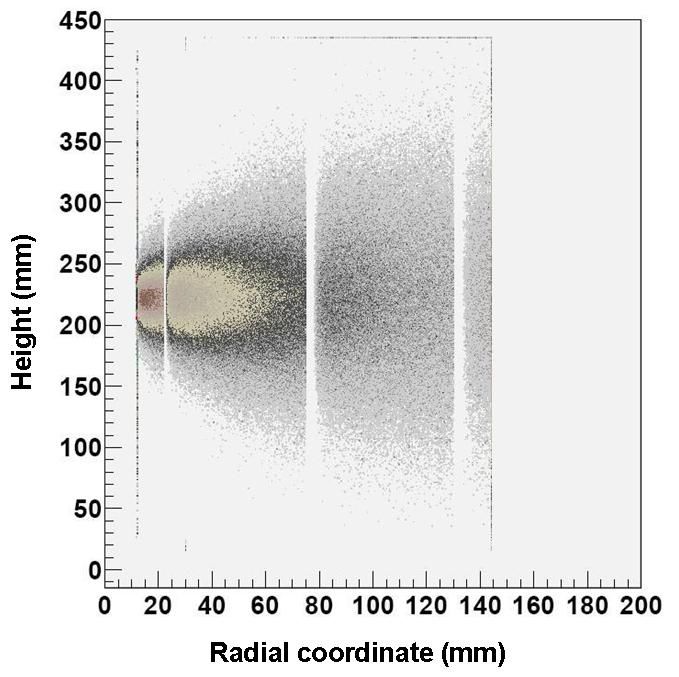
The ingredients of the charge collection algorithm are presented bellow:
the material map displays, on the grid obtained from ELMER, the distribution of
materials in the chamber (in figure 14 each material being represented with a
different color).
Figure 14: material map for the IC2010 design
the charge collection map, describes which of the components collects the charge
deposited in the gas. It can be seen, for example, that the most of the charge
deposited in the gas is collected by the two electrodes.
Figure 15: collection map for the IC2010 design
The collection volume is clearly defined, but trouble zones can be identified: the
lobes "behind" the electrode and the zone corresponding to the insulator between the
electrode and the ring.
16Figure 16: detail on the collection map for the IC2010 design
Another purpose of the charge collection map is to asses the importance of the zones
with uncertain charge collection, such as the areas behind the electrodes (where the
field is very low, but some field lines "creep in" through the distance separating the
electrodes from the guard rings) as well as the zone corresponding to the separation
between the electrodes and the guard ring, where part of the charge is collected by the
electrode and the rest by the guard ring (visible in red in the third picture, showing a
detail around the guard ring). The volume shown in green represents the volume where
the collection is uncertain, and gives an estimate of the precision of defining the
collection volume for the new design.
Results of the simulation:
1. the collection of charges does matter significantly, so for estimating the response of
the prototype a simulation (or any other type of calculation) must have a way to
describe the areas from which the charge is collected.
Figure 17: influence of the regions of non collecting charge on the response
10
Deposited energy ( keV/Bq)
1
Deposited in gas
Collected by electrodes
0.1
10 100 1000
Energy (keV)
2. the distribution of collected charge between the two electrodes: the first electrode
collects always more charge than the second. This unequal distribution of the current
between the two electrodes should be taken into account when the electrical circuits for
reading the chamber signal are designed
17Figure 18: distribution of the charge collected between the two electrodes
10
Collected Energy (keV/Bq)
1
Inner Electrode
Outer Electrode
0.1
0.01
10 100 1000
Energy (keV)
3. the insulators separating the guard rings seem appropriate, but as a design goal, they
should be as small as possible. The graph bellow shows the total charge in the non‐
collection volume between the collecting electrodes and the neighbouring guard rings.
In reality, the error on the sensitive volume will be given by only a fraction of that
volume. Additionally, in the simulation, the separation between the guard ring and
electrodes was taken as 5 mm, which could be made smaller in the prototype. An
additional observation is that for the purpose of defining the collection volume, the
insulators on the outer ring are more important than those on the inner ring.
Figure 19: precision of the volume definition in the IC2010 design
Total Volume
Inner Volume
Outer Volume
0.8
Volume definition precision (%)
0.6
0.4
0.2
0.0
100 1000
Energy (keV)
3.4.2 Two dimensional maps of the deposited/collected energy
Two dimensional maps of the deposited/collected energy were added to the
simulation to investigate the volume definition asymmetry described above and proved
a very useful supplemental test that the simulation is performing as expected. The
figures bellow present the energy deposited in the gas for a cylindrical source (ampoule)
emitting 1MeV photons. It can be seen that most of the energy is deposited around the
centre of the chamber, diminishing the effects of the trouble spaces (the lobes at the end
of the electrode and the volume corresponding to the distance between the electrode
and the guard rings for the inner ring) on the response.
18Of high interest for the project is the non‐collected volume between the inner
wall and the first collecting electrode, where a significant charge is deposited.
Figure 20: charge deposited in gas in IC2010 design
19References
1. EGS4, Electron Photon Shower Simulation by Monte‐Carlo, http://www.oecd‐
nea.org/tools/abstract/detail/ccc‐0331/ ; W.R. Nelson, H. Hirayama, and D.W.O.
Rogers, “The EGS4 code system”, Report SLAC‐265, Stanford Linear Accelerator
Center, Stanford, CA, USA, 1985.
TM
2. Briesmeister J.F., Manual MCNP ‐A general Monte‐Carlo N‐Particle Transport
Code, Version 4C, 2000; X‐5 Monte Carlo Team, “MCNP ‐ A General Monte Carlo
N‐Particle Transport Code, Version 5”, Los Alamos National Laboratory Report
LA‐UR‐03‐1987, Apr. 2003, Revised Mar. 2005.
3. PENELOPE2011, A Code System for Monte‐Carlo Simulation of Electron and
Photon Transport, http://www.oecd‐nea.org/tools/abstract/detail/nea‐1525;
Baro, J. Sempau, J. M. Fernandez‐Varea, and F. Salvat, “PENELOPE, an algorithm
for Monte Carlo simulation of the penetration and energy loss of electrons and
positrons in matter”, Nucl. Instrum. Meth. B, vol. 100, no. 1, pp. 31‐46, 1995.
4. Geant4: Nuclear Instruments and Methods in Physics Research A 506 (2003)
250‐303, and IEEE Transactions on Nuclear Science 53 No. 1 (2006) 270‐278
5. www.root.cern.ch
6. www.doxygen.org
7. http://savannah.nongnu.org/projects/cvs
8. The Geant4 Low Energy Electromagnetic Physics Working Group,
https://twiki.cern.ch/twiki/bin/view/Geant4/LowEnergyElectromagneticPhysic
sWorkingGroup
9. Elmer, Open Source Finite Element Software for Multiphysical Problems,
http://www.csc.fi/english/pages/elmer
10. "Development of an ionisation chamber for the establishment of the SI unit
Becquerel", Johan Camps and Jan Paepen, Report EUR 22609 EN
11. "An Intercomparison of Monte Carlo Codes Used in Gamma‐Ray Spectrometry" ,
APPLIED RADIATION AND ISOTOPES vol. 66 p. 764‐768
12. AZM, http://www.magnesium‐elektron.com/products‐services.asp?id=10
13. S200F, http://materion.com/~/media/Files/PDFs/Beryllium/SpecSheets/S‐
200‐F.pdf
20Additional information
Appendix 1: The configuration file
additional information for running the simulation 1. Comment line
1 2. run mode
ICsource.inp 3. Source description filename
IC2010.inp 4. Geometry description filename
ICanalysis.inp 5. Analysis description filename
0.01 6. cut-off value (mm)
vis.mac 7. default visualisation macro
CollectionMap.dat 8. collection map filename
5 9. id of the gas in the collection map
1 10. turn charge collection on (1)/off (0)
1 5 2 10 18 11. gas collection parameters
case.ep 12. elmer fields file
matMap.dat 13. material map file
The left side presents an example of configuration file. The right side is a brief
description of the field. Additional information on these can be found bellow.
1. Comment line
Can be any line of text. Can be used to describe in input file
2. run mode
Used to select the purpose of the simulation.
runMode=
1 : the normal simulation run; calculates "ICresults.root"
2 :visualisation of the geometry; execution deferred to the visualisation macro
3 : create the material map file (from the FEM‐Elmer file and geometry)
4 : create the charge collection map file (from the FEM‐Elmer file, the geometry and materials
map)
3. Source description filename
4. Geometry description filename
5. Analysis description filename
6. cutoff value (mm)
7. default visualisation macro
8. collection map filename
9. id of the gas in the collection map
10. turn charge collection on (1)/off (0)
11. gas collection parameters
id of the gas volumes in the Geant4 simulation and of the collection electrodes; format:
noOfGasVolumes listOfGasVolumes noOfCollectionElectrodes listOfCollectionElectroded
Example: a single gas volume (noOfGasVolumes=1) is used, the gas is the piece number 4
in the geometry; there are two collection electrodes, bearing number 10 and 18 in the
geometry file
12. Elmer fields file
13. material map file
21Appendix 2: Particle source file
source description in a few words: random photons from a 1. Comment line
vial; 2. shape of the source
2 3. parameters for the source shape
0 0 21.825 0 0.7645 1.0 0 0 0 0 4. number of radionuclides
14 5. radionuclide 1
4 55137 10000000 6. ….
………………. 7. radionuclide n
4 53125 10000000
The left side presents an example of source configuration file. The right side is a brief
description of the field. Additional information on these can be found bellow.
1. Comment line
2. shape of the source
1: point source:
parameters:
position: x(cm), y(cm), z(cm)
2: uniform distribution in a cylinder:
parameters:
position: x(cm), y(cm), z(cm)
size: innerRad(cm), thickness(cm), halfLenght(cm)
3. parameters for the source shape: 15 values are expected;
4. number of radionuclides
5. radionuclide 1 :
a. radionuclide code:
1. (gamma) energy (keV) activity (number to be simulated)
2. (e‐ = β‐ ) energy (keV) activity filename
3. (e+ = β+ )energy (keV) activity filename
4. radionuclide ZZAAA activity
(Z and A are used to find the file zZZaAAA.dat)
5. (e‐ = conversion electron) energy(keV) activity
22Appendix 3: Analysis file
analysis description in a few words 1. Comment line
1000000 2. No of intermediate events
0 3. TreeOutput
24 4. number of histograms
1 1000 0 200 5. objId nrBinsR lowBinR highBinR
1000 -15 450 6. nrBinsZ lowBinZ highBinZ
1000 -180 180 7. nrBinsPhi lowBinPhi highBinPhi
2 1000 0 200 8. ……….
1000 -15 450
1000 -180 180
………………….
24 1000 0 200
1000 -15 450
1000 -180 180
The left side presents an example of analysis configuration file. The right side is a brief
description of the field. Additional information on these can be found bellow.
1. Comment line
2. No of intermediate events: used for calculating the intermediate values, errors…
3. TreeOutput On(1)/Off(0)
4. number of histograms: how many histograms are being modified
5. objId nrBinsR lowBinR highBinR : the objId that has it's histogram modified and the new ranges
for (R,Z,Phi)
23Appendix 4: Geometry file
geometry description in a few words: JChamps geometry
Ar2gab 33.43 293.15 2000000 0
ArGab 33.43 273.15 2000000 0
0 1 world 0 Air 0 0 0 0 50.00 50.00 50.00 0 0 0 0 0 0 0 0 0 0 0 0 0 0 0 0 0
1 33 OutProt 0 Aluminum 1 0 0 -21.65 11.85 6.95 0.20 11.85 0.20 42.35 2.60 9.45 0.20 0 0 0 0 0 0 255255000 1 0 0 0
2 31 plasBase1 0 pvc 1 0 0 -24.05 7.00 11.80 2.40 0 0 0 0 0 0 0 0 0 0 0 0 255000255 1 0 0 0
3 31 plasBase2 0 pvc 1 0 0 19.50 2.20 8.80 1.40 0 0 0 0 0 0 0 0 0 0 0 0 255000255 1 0 0 0
4 31 pvcCase 0 pvc 1 0 0 -21.65 11.00 0.60 42.55 0 0 0 0 0 0 0 0 0 0 0 0 255000255 1 0 0 0
5 41 hold1 0 pvc 1 0 0 -1.17 0.85 0.10 0.10 0.40 1.50 7.87 9.30 0 0 0 0 0 0 0 0 255000255 1 0 0 0
6 32 suport1 0 SS 1 0 0 15.20 9.60 1.40 2.90 5.50 5.50 1.40 0 0 0 0 0 0 0 0 0 255000000 1 0 0 0
7 32 suport2 0 SS 1 0 0 -21.65 7.00 4.00 1.50 9.60 1.40 2.80 0 0 0 0 0 0 0 0 0 255000000 1 0 0 0
8 31 entry 0 vespel 1 0 0 18.10 2.00 0.20 3.00 0 0 0 0 0 0 0 0 0 0 0 0 255000255 1 0 0 0
9 33 OW 0 SS 1 0 0 -20.15 0 9.60 1.60 9.00 0.60 34.85 2.00 7.60 1.80 0 0 0 0 0 0 255000000 1 0 0 0
10 31 GasVolume 0 Ar2MPa 1 0 0 -18.55 2.20 6.80 34.85 0 0 0 0 0 0 0 0 0 0 0 0 0 0 0 0 0
11 32 Electrode 10 Aluminum 1 0 0 -13.26 5.40 1.30 0.50 5.40 0.20 28.15 0.00 0.00 0.00 0 0 0 0 0 0 255255000 0 0 0 0
12 31 guardRing 10 Aluminum 1 0 0 -15.43 3.55 4.50 0.20 0 0 0 0 0 0 0 0 0 0 0 0 255255000 0 0 0 0
13 31 IW 0 Aluminum 1 0 0 -18.55 2.00 0.20 34.85 0 0 0 0 0 0 0 0 0 0 0 0 255255000 0 0 0 0
14 23 AmpGlas2 0 G4_GLASS_PLATE 1 0 0 -1.00 0.76 0.30 0.44 0.30 3.46 4.16 4.86 5.43 6.80 0 0 0 0 0 0 120120120 0 0 0 0
15 31 AmpLiquid 0 G4_WATER 1 0 0 -1.00 0 0.76 1.00 0 0 0 0 0 0 0 0 0 0 0 0 120120255 0 0 0 0
id shape name m material s x y z 1 2 3 4 5 6 7 8 9 10 11 12 13 14 15 color v 1 2 3
Position Parameters of the shape Orientation
1. id: identification number of the object
2. shape code (described bellow)
3. name
4. id of mother object
5. material
6. sensitive (1) or not sensitive (0) object
7. x,y,z: position of the object
8. 1‐15: numerical values of the parameters defining the shape
9. RGB color code of the object
10. visible(1) or not (0) in visualisation
11. G1‐G3: orientation of object in space(arbitrary rotation in space is possible)
24The shape codes
The shape codes (shapeID) are the codes of the building blocks making up the structure
of the ionisation chamber. The meaning of the shape codes can be found bellow.
1. Box: shapeID= 1; parameters: halfLenghtX(cm), halfLenghtY(cm),
halfLenghtZ(cm);
2. source ampoule
a. shapeID= 21 shape 1 (flat bottom, straight neck):
b. shapeID= 22 shape 2 (flat bottom, shaped neck, neck dimensions relative
to the other dimensions)
c. shapeID= 23 shape 3 (taken from J.Champs MCNP simulations)
2. Tube: 3 types of tube have been implemented: 31 ‐ T1, 32 ‐ T2, 33 ‐ T3
253. source holder
a. shapeID=41
Materials
The materials used by the existing prototype or expected to be used by the
prototype were hardcoded in the simulation. On top of those, the NIST materials
database can be used (for example G4_WATER denotes water, as described by NIST).
26Sensitive components
Geant4 allows a separation between the structural components and the sensitive
ones. The sensitive components are those whose interactions are being analysed.
This parameter is set to 1 if the component is active for detection, and 0 if it is a
structural component.
In a real ionisation chamber the only sensitive component is the pressurised gas, but
the simulation allows the study of energy loss in each of the components. In the example,
all the components are declared as sensitive, so that the energy loss in each of them can
be studied.
RGB code and visualisation
Geant4 allows the rendering of the geometry of the detector on a number of graphic
interfaces for the purpose of "debugging" the geometry. This 3D representation becomes
complicated when all the components are visible, so switches were implemented to
toggle the visibility of the different objects. The 9 digits RGB colour code sets the colour
that the object will have in the representation (RRRGGGBBB).
27Appendix 5: Precision of the simulation
Calculating the energy deposited in each component is only the first step in obtaining
meaningful results from the Monte Carlo simulation. The Geant4 framework does not
supply the means to analyse the accuracy and precision of the energy deposits, but
provides an easy mean for them to be developed by the user, as part of the analysis. In
this respect, the strength of the Geant4 framework lies in that it gives full access to the
information about each hit in the detector.
Notations:
detector: one sensitive component in the Geant4 geometry
xi is the energy deposited in one detector during an event (During each event,
there might be more interactions in the same detector, depending on the
complexity of the event/detector. If this is the case, xi is the sum of these energy
deposits)
N is the number of events that were simulated
Sj=Σ(xi)j are the sums of the different energy depositions, updated after each
event.
With these notations, the following values are calculated:
Mean=S1/N : the mean energy deposited during one event
SDev=S2/N‐Mean2 : the standard deviation of the energy deposits during one
event
MeanSDev=SDev2/N : the standard deviation of the mean
RelErr = MeanSDev/Mean : the relative error of the mean
VoV=(S4‐4S1S2/N + 8 S2S12/N‐4S14/N3‐S22/N)/(S2‐S12/N)2 : the variance of
variance
In principle, these values can be calculated (and saved) after each event, but this would
generate a very high amount of (useless) information, if we are taking into account that
the number of events in a simulation is of the order of 106. To bypass that, a parameter
was included in the analysis configuration file of the simulation that decides how often
this value to be calculated and saved. They are always calculated at the end of the
simulation.
Note: these precision estimates are replicating the method used by MCNP and described
in chapter IV of the manual: "Estimation of the Monte Carlo precision"
28Appendix 6: Charge collection
Simulating the charge collection in the ionisation chamber requires the knowledge of the
(stationary) electrical fields that are present when the chamber is in operation, the
knowledge of where the interaction takes place (starting point for the movement of
charges) and a possibility to check, after each of the iterative steps if the charged
particle has reached the boundary of the gas. In principle, none of these steps is
performed using the Monte‐Carlo method, but nonetheless, performing the charge
collection as part of the simulation has clear advantages: the start point of the track is
generated by the simulation, and the geometry can be interrogated to decide if the
charge cloud has reached the boundary. Tracking is performed assuming that all the
charge cloud moves through the gas a single particle.
In practical terms the following steps are to be followed to implement the charge
collection:
1. define the geometry of the chamber
2. identify the 2D part that is to be used in the fields calculation
3. run the fields calculation using ELMER
4. run the simulation to create the materials map ( interrogates the Geant4 geometry
about what object contains each of the fields grid nodes)
5. run the simulation to create the collection map (an optimisation step; most of the
space in the collection volume will be collected by the electrodes, so at this point for
each node of the grid a charge is created and tracked; the cells where the adjacent nodes
are collected by the same electrode will be collected by the same electrode)
6. run the simulation (only the interaction points at "difficult" positions according to the
collection map are tracked, the rest are taken from the collection map).
Notes on the implementation:
the grid used in ELMER must be rectangular
the fields inside the cells are calculated by bilinear interpolation
the charges are propagated from interaction to first intersection with the grid,
then from grid line to grid line
the collection is stopped when either the charge takes too long to be collected
(is in a low field area) or when it exits the gas;
29European Commission
EUR 25676 EN --
- Joint Research Centre --
- Institute for Reference Materials and Measurements
Title: Report on the Geant4 simulations performed for the "Realisation of the Bq" project
Author(s): Gabriel Suliman
Luxembourg: Publications Office of the European Union
2013 --- 29 pp. --- 21.0 x 29.7 cm
EUR --- Scientific and Technical Research series --- ISSN 1831-9424 (online)
ISBN 978-92-79-28074-0
doi:10.2787/70585
Abstract
Monte Carlo simulations have become an integral part of developing new radiation detectors and the work on the
ionisation chamber that is being built as part of the project "Realisation of the Bq" makes no exception. Until now, Monte
Carlo simulations were performed at IRMM using EGS4 and MCNP5 and at LNHB using Penelope. Some of these
simulations were used to define the parameters of a prototype ionisation chamber, while others dealt with other aspects
of the operation of the chamber such as the effect of the ampoules holding the source, or the positioning of the ampoule.
In 2010 the work started on designing a new prototype. At the same time, a new simulation program for the project was
started, using the Geant4 framework.
This technical document presents the details of the simulations as they were performed using the Geant4 framework,
focusing on the last version of the simulation code. This document, together with the source code and the documentation
included in the source code should provide enough information for anyone to reproduce the results and expand the
simulations.z #
LA-NA-25676-EN-N
As the Commission’s in-house science service, the Joint Research Centre’s mission is to provide EU
policies with independent, evidence-based scientific and technical support throughout the whole policy
cycle.
Working in close cooperation with policy Directorates-General, the JRC addresses key societal
challenges while stimulating innovation through developing new standards, methods and tools, and
sharing and transferring its know-how to the Member States and international community.
Key policy areas include: environment and climate change; energy and transport; agriculture and food
security; health and consumer protection; information society and digital agenda; safety and security
including nuclear; all supported through a cross-cutting and multi-disciplinary approach.You can also read