Stimulated Raman Scattering Simulation for Imaging Optimization

Stimulated Raman Scattering Simulation for
Imaging Optimization
Liron Zada (  lironzada@gmail.com )
 Vrije Universiteit Amsterdam https://orcid.org/0000-0002-8419-1945
Bart Fokker
 Vrije Universiteit Amsterdam
Heather A. Leslie
 Vrije Universiteit Amsterdam
A. Dick Vethaak
 Vrije Universiteit Amsterdam
Johannes F. de Boer
 Vrije Universiteit Amsterdam
Freek Ariese
 Vrije Universiteit Amsterdam

Research

Keywords: Raman, Simulation, Imaging, Optimization, Resolution, Microscopy, Non-linear, Multiplex, Lock-
in ampli er, Modulation

Posted Date: November 18th, 2020

DOI: https://doi.org/10.21203/rs.3.rs-99940/v1

License:   This work is licensed under a Creative Commons Attribution 4.0 International License.
Read Full License

Version of Record: A version of this preprint was published at Journal of the European Optical Society-
Rapid Publications on June 16th, 2021. See the published version at https://doi.org/10.1186/s41476-
021-00155-w.

1 Stimulated Raman scattering simulation for imaging

 2 optimization

 3 Liron Zada1,2, Bart Fokker1, Heather A. Leslie2, A. Dick Vethaak2,3, Johannes F. de Boer1, Freek

 4 Ariese1*

 5 Affiliations:
 1
 6 LaserLab Amsterdam, Department of Physics and Astronomy, Faculty of Sciences Vrije

 7 Universiteit Amsterdam, De Boelelaan 1081, 1081 HV Amsterdam, The Netherlands.

 2
 8 Department of Environment and Health, Vrije Universiteit Amsterdam, De Boelelaan 1085,

 9 1081 HV Amsterdam, The Netherlands.

 3
10 Deltares, Marine and Coastal Systems, P.O. Box 177, 2600 MH Delft, The Netherlands.

11 *Correspondence:

12 Liron Zada

13 LaserlaB Amsterdam, Department of Physics and Astronomy, Faculty of Sciences Vrije

14 Universiteit Amsterdam, De Boelelaan 1081, 1081 HV Amsterdam, The Netherlands

15 Telephone number: +31 20 59 85425

16 Email: lironzada@gmail.com

 1

17 Abstract

18 Two simulation programs of a stimulated Raman scattering microscopy (SRS) imaging system

19 with lock-in amplifier (LIA) detection were developed. SRS is an imaging technique based on

20 the vibrational Raman cross-section as the contrast mechanism and enables fast, label-free

21 imaging. Most SRS implementations are based on a LIA detection of a modulated signal.

22 However, building and operating such SRS set-ups still poses a challenge when selecting the

23 LIA parameter settings for optimized acquisition speed or image quality. Moreover, the type of

24 sample, e.g. a sparse sample vs. a densely packed sample, the required resolution as well as the

25 Raman cross-section and the laser powers affect the parameter choice.

26 A simulation program was used to find these optimal parameters. The focal spot diameters of

27 the individual lasers (pump and Stokes) were used to estimate the effective SRS signal focal spot

28 and the (optical) spatial resolution. By calibrating the signal and noise propagation through an

29 SRS system for a known molecule, we estimated the signal and noise input to the LIA. We used

30 a low pass filter model to simulate the LIA behavior in order to find the optimal parameters (i.e.

31 filter order and time constant).

32 Optimization was done for either image quality (expressed as contrast to noise ratio) or

33 acquisition time. The targeted object size was first determined as a measure for the required

34 resolution. The simulation output consisted of the LIA parameters, pixel dwell time and contrast

35 to noise ratio.

36 In a second simulation we evaluated SRS imaging based on the same principles as the optimal

37 setting simulation, i.e. the signals were propagated through an imaging system and LIA

 2

38 detection. The simulated images were compared to experimental SRS images of polystyrene

39 beads.

40 Finally, the same software was used to simulate multiplexed SRS imaging. In this study we

41 modeled a six-channel frequency-encoded multiplexed SRS system demodulated with six LIA

42 channels. We evaluated the inter-channel crosstalk as a function of chosen LIA parameters,

43 which in multiplex SRS imaging also needs to be considered.

44 These programs to optimize the contrast to noise ratio, acquisition speed, resolution and

45 crosstalk will be useful for operating stimulated Raman scattering imaging setup, as well as for

46 designing novel setups.

47 Key words:

48 Raman, Simulation, Imaging, Optimization, Resolution, Microscopy, Non-linear, Multiplex,

49 Lock-in amplifier, Modulation.

50 Introduction

51 Stimulated Raman scattering microscopy (SRS) is a non-linear imaging modality with a

52 spectral response similar to spontaneous Raman scattering. Compared with spontaneous Raman,

53 SRS offers an increase in mapping speed of several orders of magnitude. Unlike spontaneous

54 Raman, SRS is not affected by background fluorescence. SRS is realized by two laser beams that

55 directly probe a specific vibrational state of a molecule if their photon energy difference matches

56 the energy of a vibrational transition. Then the SRS signal can be detected as a gain in intensity

57 of the low energy beam (stimulated Raman gain of Stokes) and a loss in the high energy beam

58 intensity (stimulated Raman loss of pump)1.

 3

59 SRS, as a fast imaging modality, was first demonstrated by Freudiger et al.2 and others3,4 with

60 the introduction of an amplitude modulation of one of the laser beams and demodulation by a

61 lock-in amplifier (LIA) for detection and noise filtering. Modulation at high frequency allowed

62 the rejection of the lasers’ relative intensity noise (RIN) which dominates at frequencies below 1

63 MHz. A combination of a high modulation frequency, where the laser noise is low, and laser

64 powers at which the shot-noise surpasses the thermal noise, results in shot-noise limited

65 detection. After the probe beam is detected (e.g. the pump beam in stimulated Raman loss),

66 demodulation of the signal takes place by means of a LIA or alternatively home built electronics

67 (e.g. tuned amplifier5). Throughout this paper, we choose not to use the common convention of

68 Stokes and pump beams to keep the discussion general. Instead, we refer to the amplitude

69 modulated beam as the carrier, as it carries the amplitude modulation, and to the detected beam

70 as probe.

71 While the modulation frequency is mentioned as an important parameter in most studies, only a

72 few studies5–7 discussed the (low pass) filter bandwidth, which is an important parameter that

73 affects the acquisition speed and noise. Specifically for the LIA in the context of SRS, to the best

74 of our knowledge no in-depth analysis has been reported for the input parameters of the filter

75 bandwidth. While most SRS studies mention the time constant (TC), almost none8 mention the

76 equally important filter-order (n), which makes it impossible to calculate the bandwidth or

77 compare modalities reported in the literature. Since the conventional imaging manner of non-

78 linear modalities, such as SRS, is scanning the focal spot across the sample, the scanning speed,

79 the filter response, the focal spot size, and the spatial resolution in the scanning direction are

80 related. Thus, for an object of a given size and with the theory of the LIA filter response for a

81 given bandwidth, one can extract the optimal settings needed for imaging this object with SRS,

 4

82 either with regard to the signal to noise ratio (SNR), contrast to noise ratio (CNR)9–11 or to the

 83 acquisition speed.

 84 Here, we describe the operation principle of LIAs, and investigate the signal and noise

 85 propagation in the time and frequency domain. Then, we link this to the physical properties of an

 86 SRS setup, such as laser powers, focal spot size and pixel dwell time (PDT), in order to optimize

 87 the SRS imaging. The optimization procedure is compiled into a simulation program in order to

 88 address different imaging scenarios: optimization for CNR or imaging time in a sparse or tightly

 89 packed sample. The rational for the optimization for CNR, rather than SNR, is explained in the

 90 optimal settings simulation part in the results section. A detailed description of the input and

 91 output parameters of the software’s user interface is given in the optimal settings simulation

 92 section and in the supplementary material.

 93 Furthermore, we generalize this result in order to demonstrate extended capabilities of this

 94 analysis. An additional simulation with a visual output (called imaging simulation) was created,

 95 based on the same LIA theory and input parameters. This simulation provides a qualitative image

 96 visualization, either for narrowband SRS, or for a multiplex SRS setup that has multiple

 97 modulated bands and multiple detection channels. As a test case, we analyze a simulated

 98 frequency channel encoded multiplex SRS setup as demonstrated before12,13, however in our

 99 simulation the signal is demodulated with a multi-channel LIA. Here, crosstalk between channels

100 is also treated, in addition to resolution, CNR and acquisition speed.

101 Theory: parameters of the lock-in amplifier

102 The SRS signal is a small modulation carried on a large background. This large DC background

103 is the source for the laser RIN and shot noise. In the LIA this large DC background is filtered

 5

104 out, and the small modulation is mixed with a reference frequency. Then, the signal amplitude is

105 recovered by applying a low-pass filter, here modeled as a discrete time RC filter, which is an

106 exponential running average filter14:

107 (1)

108 Where k is the index of the processed sample Xout at specified discrete sampling times Ts. Thus,

109 every Xout is a weighted averaged between the new input Xin and the previous sample Xout of k-1.

110 It is possible to cascade these filters such that the signal and noise pass through multiple filters.

111 The number of filters is called the filter order (n). The frequency domain response of the filter

112 with TC and n is described as:

113 (2)

114 Where Δf is the difference between modulation frequency and the detection frequencies; the

115 input frequencies to the LIA. The filter transmission which describes the signal propagation

116 through such a filter is then:

117 (3)

118 Measurements that verify this model in the frequency and time domain are provided in Figure

119 S1 in the supporting information.

120 The possible noise sources in SRS are the thermal (Johnson–Nyquist) noise from the different

121 electronic components, the shot noise from the detected (probe) laser light and the frequency

122 dependent RIN15 from the laser source of the probe light. While the thermal noise is independent

123 of the probe power, the shot noise is proportional to the square-root of the probe power. We

124 ignored the RIN in our analysis for two reasons. One was the assumption that thermal or shot

 6

125 noise limited systems cover most scenarios for SRS imaging, and provides a sufficient

126 description for our analysis. The second was that our experimental system is either thermal or

127 shot noise limited. Since the detection frequency is above 1 MHz, the RIN is small compared

128 with the thermal or shot-noise for the power range that was used. With increasing powers, the

129 photo-detector saturates before RIN dominates the noise over thermal or shot noise (Figure S2d).

130 For the thermal and shot noise contributions, the propagation of the noise from the detector

131 through the LIA is determined by the bandwidth of the filter. A useful expression for the

132 quantification of the noise bandwidth is the noise equivalent power bandwidth (NEPBW, Figure

133 S2a), which assumes a flat (white) noise spectrum. It is modeled as a rectangular-shaped filter,

134 which lets the same amount of noise power pass as the actual filter. The flat noise spectrum

135 assumption is valid for small bandwidths relative to any large non-flatness in the spectrum

136 caused by electronic components (e.g. photo-diode or trans-impedance amplifier). The NEPBW

137 is derived from the discrete time RC filter, and is therefore described by the same TC and n

138 parameters. Integration of the square of the filter transmission (Eq. 3) gives:

139 (4)

140 Where the filter order n is expressed through the gamma function. The NEPBW has frequency

141 units (Hz).

142 Results

143 Calibration of signal and noise

144 For the calibration of our system we used the Raman signal of a polystyrene (PS) bead as a test

145 sample at 1602 cm-1. The signal calibration coefficient Csig is defined as the product of the

 7

146 Raman cross-section of PS and the number of molecules in the focal volume, propagated through

147 the collection optics and the detection electronics (photo detector, trans impedance amplifier and

148 LIA). If we wish to use this result for another analyte than PS, we simply have to determine the

149 ratio between the signals generated by both analytes on our system (i.e. convert the cross-section

150 from one to another). Accordingly, CTN, CSN are the thermal and shot noise calibration

151 coefficients, which are independent of the analyte cross-section in SRS:

152 (5)

153 (6)

154 (7)

155 where Sps is the signal generated by PS and is measured in Volts at the output of the LIA, Pc is

156 the average intensity of the modulated carrier and Pp is the intensity of the probe in milli-Watts.

157 In addition, NT and NS are the noise contributions of the thermal noise and the shot noise,

158 respectively, which are given in Volts. The calibration coefficients were extracted from a fit to

159 the measurements shown in Figure S2c for the signal and S2d for the noise contributions. In

160 these measurements the ratio between the carrier and the probe power was always set to 2:116,

161 which is reflected in the slope of 2 in the signal graph (Figure S2c) that it follows from the

162 product of the carrier and probe powers. From the linear part of that slope we extract the

163 coefficient Csig following equation (5). The slope of the shot noise region in the noise graph as a

164 function of probe power in Figure S2d follows a square root relation to the probe power, and is

165 an indication that the system is indeed shot noise limited when using these powers as explained

166 in Figure S2b. The coefficient CSN is derived from the slope of Figure S2d, following equation

167 (7), and CTN is calculated from equation (6), where NT is measured with no light on the detector.

 8

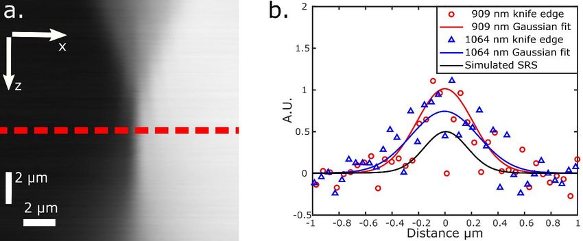
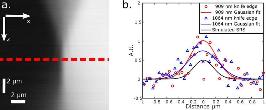
168 These coefficients are used as default input to the simulations explained below, but can be

169 changed to fit a simulation of any SRS system:

170 Csig=3×10−6 / 2, CTN=1.518 × 10−7 /√ and CSN=1.36 × 10−7 /√( ).

171 Focal spot size and optical spatial resolution

172 In order to relate the LIA performance with different settings to imaging parameters of a given

173 object, the focal spot size of SRS has to be considered. Since the SRS signal is the product of

174 two beam intensities, the effective focal spot intensity profile of SRS is the product of the carrier

175 and probe beams’ focal spot profiles. Assuming both have a Gaussian intensity profile and are

176 slightly underfilling the objective’s back aperture17,18, we can approximate both beams to have a

177 Gaussian profile at the focal plane and their product will be a Gaussian as well. The resulting

178 product beam width or SRS beam full width at 1/e2, ωSRS, is described by equation (8)19:

179 (8)

180 The focal spot widths of the carrier and the probe beams were measured by a knife-edge

181 measurement, taking the derivative of the intensity profile and fitting it to a Gaussian. Since sub-

182 micron widths were expected, we used a USAF target to replace the knife. This was repeated at

183 various z depths. An X-Z intensity profile of the 1064 nm beam is shown in Figure 1a for

184 illustration (with x being the scanning direction and z as the depth); the dashed red line indicates

185 the depth of the steepest measured intensity profile. The derivative of each line at different

186 depths was fitted to a Gaussian from which the beam widths were extracted. The minimum of

187 these widths was found by fitting a parabola. The effective SRS beam width was determined as

188 described by equation (8). Figure 1b shows the smallest widths from knife edge measurements of

 9

189 the carrier and the probe with a Gaussian fit. The resulting 1/e2 width is 0.89 µm for the probe

190 focal spot size and 1.03 µm for the carrier focal spot size. Accordingly, the SRS beam effective

191 spot size width is 0.67 µm. Following the resolution derivation for a Gaussian beam

192 approximation as described in the supplementary information (Eq. S2-S4)20–22 we get the SRS

193 Rayleigh resolution as 1.03∙ωSRS= 0.69 µm.

194

195 Figure 1: A measured beam profile at 1064 nm is shown in (a) to illustrate the result of one

196 beam knife edge measurement in the lateral and the axial (depth) directions indicated by x and

197 z, respectively. The dashed red line indicates the steepest slope, i.e. the focal plane depth.

198 Derivatives of the measured data of the beam profiles at the focal plane are shown in (b) for

199 the probe at 909 nm (red line) and the carrier at 1064 nm (blue line). Multiplying the fitted

200 Gaussians of the two beams gives the SRS profile also shown in (b) (black line). Note: 1. One

201 fourth of the data points are plotted for clarity. 2. SRS beam profile not to scale on the y-axis.

 10

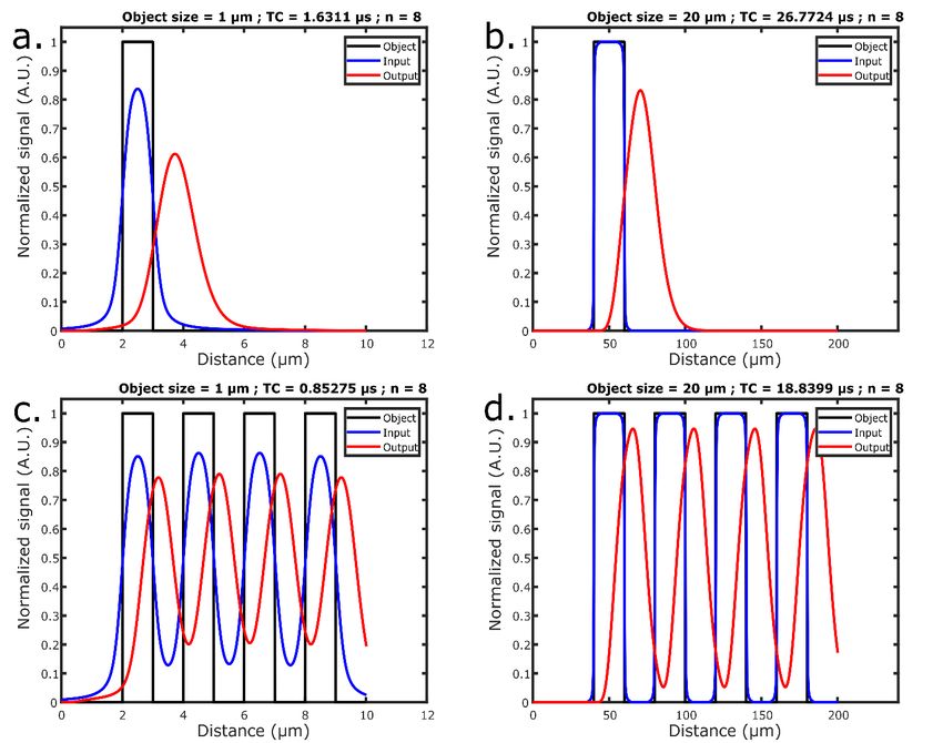
202 Optimal settings simulation

203 The optimal settings simulation gives the LIA’s filter order and time constant optimal values.

204 In order to properly simulate the SRS imaging behavior, we have to consider first the physical

205 input parameters of the imaging system. The input signal is given by equation (5), and only

206 requires the laser powers as input, given that Csig is calibrated. Upon calibration of CTN and CSN,

207 the noise contributions can be simulated as well for each TC and filter order with equation (6)

208 and (7) and the NEPBW expression in equation (4). For the optical point spread function (PSF),

209 the required input is the 1/e2 radius of the probe and carrier beams and equation (8). A detailed

210 description of the input parameters and the setup parameters is given in Figure S3.

211 Simulation of the lock-in parameters is done with respect to an object size input. The object is

212 modelled as a top-hat (black lines in Figure 2) with a width of the object size and a height of the

213 signal SPS (Eq. 5). First, it is convolved with the PSF (blue lines in Figure 2), which we derived

214 from the SRS signal effective spot size. Then, using the convolution of the input object with the

215 PSF, the input signal in discrete time steps is determined by equation (1) (red line Figure 2). The

216 signal propagation in time translates into a spatial signal propagation by the scanning speed,

217 which is simply the pixel size divided by the pixel dwell time.

218 The LIA parameters are then optimized by running this simulation multiple times over a range

219 of TCs and filter orders, optimizing for either imaging time (for a given CNR), or CNR (for a

220 given imaging time). The CNR9–11 is calculated as follows:

221 (9)

 11

222 where Ipeak is the signal value at the apex of the output curve, and Ivalley is the value at a local

223 minimum between two apexes in a dense sample case (red lines in Figures 2c-d). In the sparse

224 sample case, the Ivalley is zero (red lines in Figures 2a-b). The noise, however, is the same

225 everywhere in SRS, as it is independent of the signal, but rather depends on the probe laser

226 power as illustrated in Figure S2b. The CNR is the difference between two signals with a similar

227 noise level, so there is an additional √2 factor in the dominator compared with the SNR, which is

228 simply dividing the signal by the noise. In both cases, CNR is a single term giving a description

229 of the quality of the signal (like SNR15) as well as a measure to distinguish an object from its

230 surrounding (like contrast).

231 Different lock-in parameters are tested to find the combination that yields the shortest imaging

232 time or the maximum CNR, respectively. This can be done either for a sparse sample (single

233 particle) case or a dense sample case (tightly packed particles). In a dense sample, the object size

234 represents both an object size and the gap between two objects, i.e. the spatial resolution is half

235 of the object’s reciprocal (in units of line-pairs per millimeters).

236 The simulation produces plots (Figure 2) to illustrate the signal propagation of a given object in

237 terms of signal response and delay. The LIA setting filter order and TC are in the title of these

238 plots. The full output parameters, like the CNR, filter order, time constant and PDT are then

239 shown in the user interface (see Figure S3).

240 As an example, we tested the response for a PDT as short as 10 µs, for an object in a dense

241 sample with 1 µm object size and 1 µm pixel size. In this test case the maximum CNR was 4.6,

242 found for a TC of 0.85 µs and a filter order of n=8 (see figure 2c).

 12

243 Alternatively, the simulation can also optimize the lock-in parameters to find the minimum

244 imaging time for a specified CNR, which is calculated the same way as described above. In this

245 case, the shortest PDT is chosen for the optimal TC-filter order combination. For the same test

246 case above, first setting CNR=2, we get PDT = 2.7 µs, TC=0.23 µs with filter order n=8 as the

247 parameters that give the shortest imaging time for a minimum required spatial resolution in the

248 scanning direction.

249

250 Figure 2: The user interface of the SRS optimal parameters simulation is shown in Figure S3. The

251 power input was 24.7 mW for the carrier and 14.6 for the probe on the sample, respectively.

252 Pixel dwell time was set to 10 µs. A visualization of the signal response through the simulated

 13

253 system of a CNR optimized case, excluding the noise, is shown in (a) for a single object size of 1

254 µm and in (b) for an object size of 20 µm. In (c) and (d) a simulation is shown for a dense sample

255 with an object size of 1 µm and 20 µm, respectively. The object size represents the half period

256 distance of the spatial modulation, (i.e. it accounts for both the particle and the gap between

257 particles in a dense sample).

258 Imaging simulation compared with SRS imaging

259 The same LIA’s filter response in equation 1 in combination with the calibrated signal and

260 noise terms (Eq. 5-7) and the PSF (Eq. 9) can be used for visualizing SRS imaging. The imaging

261 simulation receives the aforementioned system and imaging parameters as input together with an

262 one-dimensional or two-dimensional object input. The result is a simulated image of an object

263 passing through the SRS imaging system. Possible input objects are one dimensional top hat

264 object, one dimensional square wave, and two-dimensional round objects to simulate beads. For

265 example, beads imaged with SRS are compared with simulated 2D beads images in Figure 3,

266 both with the same system and imaging parameters.

267 The imaging simulation creates an image using the input objects and input parameters as

268 follows. Firstly, the shape of the object is convolved with the PSF. Secondly, the object is scaled

269 by the beam powers according to equation (5) to form the input signal and the noise is added

270 (Eq. 6 and 7). Finally, the object is passing through the low-pass filter as described by equation

271 (1) by virtual horizontal scanning (left to right). A description of the imaging simulation

272 interface, with different input parameters and setup options, is given in the Supplementary

273 Material, Figure S5.

 14

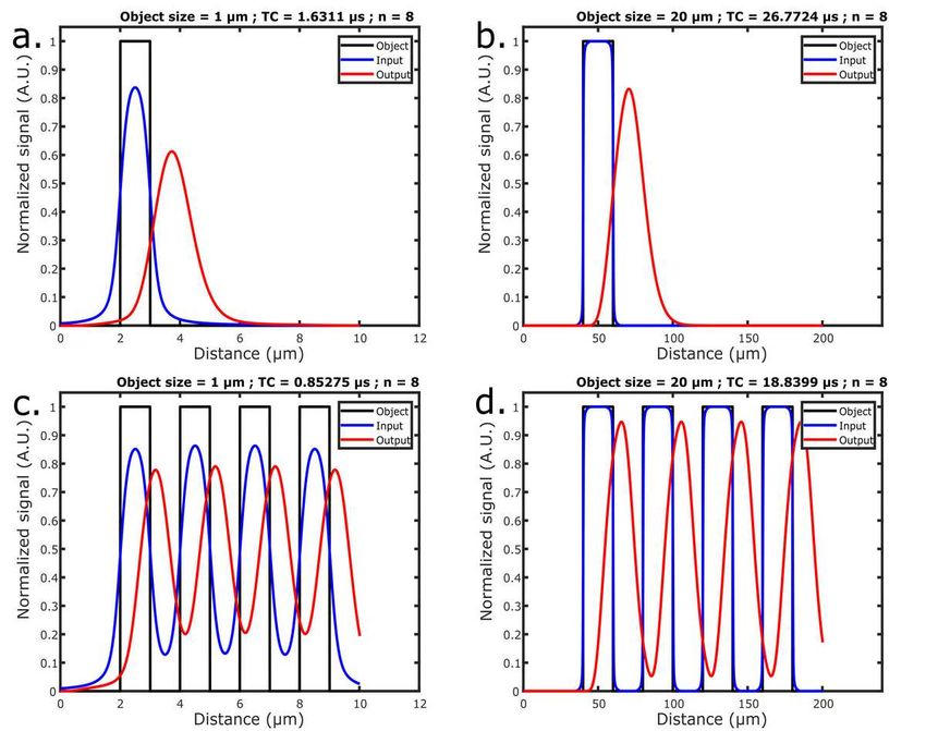
274 The results in Figure 3 demonstrate the principles discussed in the ‘Optimal setting simulation’

275 section. Figures 3a and 3b show images from measurements and simulation of a 20-µm bead,

276 respectively, optimized for a single object size of 1 µm, with a good spatial resolution and high

277 noise as shown by the profile insets. Doing the same in Figures 3c and 3d with an optimization

278 for 20 µm objects reduces the noise due to the slower response of the filter (with a narrower filter

279 bandwidth), but also reduces the signal’s peak height in the measured bead image. The

280 simulation automatically scales the signal to cover the whole dynamic range. Nevertheless, both

281 in measurement and simulation, optimization for 20 µm results in a better CNR, which allows us

282 to detect this single object better in an image with a given PDT, albeit blurred. The resulting

283 CNR values, together with the optimized lock-in parameters are listed in Table 1. Additionally,

284 the slower filter response leads to a noticeable horizontal displacement of the objects, as seen in

285 Figures 3c and 3d compared with Figures 3a and 3b.

286

287 Figure 3: Imaged and simulated beads with intensity line profiles of 60 µm in the insets. The top

288 row are 20 µm beads imaged with carrier and probe powers of 24.7 mW and 14.6 mW,

 15

289 respectively. The lock-in settings were optimized for an object size with the optimal settings

290 simulation: (a) for 1 µm, (c) for 20 µm, (e) for 2 µm, (g) for 20 µm. The bottom row (b, d, f and

291 h, respectively) are beads simulated with the same parameters and applied powers. The four

292 left-hand side images (a, b, c and d) are imaged and simulated with the single object criteria,

293 and the right-hand side (e, f, g and h) for the tightly packed sample criteria.

294 Table 1: comparison of CNR values of images in Fig. 3 that were imaged and simulated with

295 settings obtained from optimal setting simulation.

 single 1 µm object; single 20 µm object; dense sample 2 µm; dense sample 20 µm;
 CNR values TC=1.6 µs; n=8 TC=26.5 µs; n=8 TC= 1.8 µs; n=8 TC=18.7 µs; n=8

 Imaged: 9.3 20.7 9.0 6.3

 Simulated: 7.3 25.4 8.1 5.4

296

297 Figures 3e-h show images of 2 measurement–simulation-pairs of two beads separated by 2 µm.

298 One pair was optimized for a 2 µm object in a dense sample (Fig. 3e and 3f), and the other for a

299 20 µm object (Fig, 3g and 3h). In the latter case, the slower filter response leads to a lower noise

300 level, but also to a less deep signal in the gap between the beads, which counteracts any

301 improvement of the noise level. Thus effectively, the CNR decreases (see Table 1).

302 Multiplex SRS imaging simulation

303 The imaging simulation was generalized to provide not only a visualization of a narrowband

304 imaging system, but also multiplexed SRS imaging approaches. In this section, we simulated and

305 investigated settings for a multiplex SRS system, with modulation encoded channels and a single

306 detector. This analysis of frequency encoded multiplex SRS also considered the channels’

 16

307 spacing, i.e. the separation between adjacent channels in the frequency domain. This is done in

308 order to avoid crosstalk on a limited detection bandwidth while still optimizing for CNR or

309 acquisition speed.

310 We use the same imaging simulation described in the previous section to investigate an

311 imaging approach for the detection of multiple bands at the same time. It is a frequency-encoded

312 multiplex SRS approach, similar to the work done by Liao et al. in 20157. Here we name it

313 ‘single carrier modulation’. In this approach, a combination of a narrowband and a broadband

314 laser beam is used, where the narrowband is used as a probe. The broadband beam is divided into

315 different spectral bands. Each band, that we also call channel, is being modulated at a different

316 frequency. As a result, this multiplex SRS approach has many carriers, while only one probe is

317 used. After the sample, the modulation is transferred to the probe by the SRS process. The probe

318 is then measured by a single detector. Other multiplexing options are shown in the user interface

319 (Figure S5).

320 In multiplex SRS, the low pass filter bandwidth plays a role not only in determining the signal

321 and noise propagation, but also for the crosstalk between the channels. In our experimental setup

322 we used a trans-impedance amplifier to amplify the signal around the modulation frequency. The

323 trans-impedance amplifier has a bandwidth of 43.5 kHz around 3.63 MHz, with an amplification

324 of above 99% of the original amplification of 86 dB. This means that the measured calibration

325 coefficients (Eq. 5-7) provide a good approximation that can be used for the multiplex simulation

326 within that bandwidth. In this section we simulated multiple beads at 6 different modulation

327 channels, modeling samples of different materials. For simplicity, all Raman cross-sections were

328 set to that of the 1602 cm-1 band of polystyrene. The frequency separation between adjacent

329 channels was 8.7 kHz to fit the 6 channels in the aforementioned bandwidth.

 17

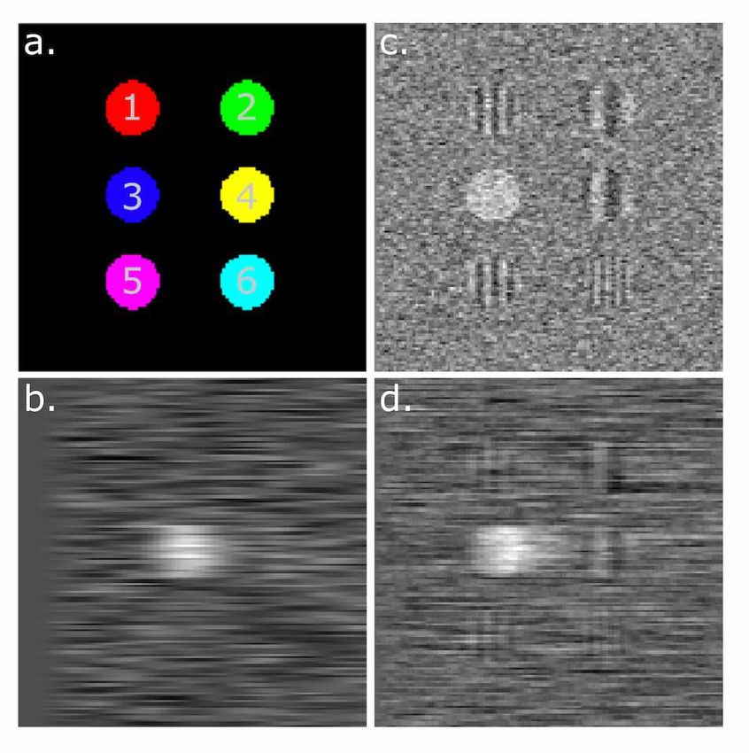
330 In Figure 4, we show the results of simulations with 3 TC settings, for a hypothetical situation

331 of six different beads of 20 µm diameter, where each bead is in a different channel. Fig 4a is a

332 schematic image showing the beads. Figure 4b is a simulated image with settings optimized for a

333 20 µm object (bead #3 in blue in Fig. 4a) in a sparse sample, which results in no crosstalk; note

334 the horizontal displacement due to the slow filter response. Fig. 4c is an image using parameters

335 optimized for 1 µm, which shows a sharper image but also crosstalk in channel 3 from other

336 channels. Fig. 4d shows the results with filter order 1 and time constant 125 µs, which

337 theoretically should result in the same CNR as in 4b, since these settings have the same NEPBW

338 as in 4b. However, due to the less steep filter shape of filter order 1 than filter order 8, there is

339 more crosstalk from neighboring channels.

340 These results can be understood through the filter transmission (Eq. (3)). If a channel’s

341 bandwidth is larger than the frequency distance between neighboring channels, the signal from a

342 neighboring channel will appear as an oscillation modulated at the frequency difference of the

343 channels (i.e. beating frequency at Δf). By multiplying the transmission of the channel at Δf,

344 with the signal strength at the neighboring channel (Eq. 5), we get the value for the amplitude of

345 this crosstalk oscillation.

 18

346

347 Figure 4: Simulation of 6 channels over a band of 43.5 kHz; 8.7 kHz separation between

348 neighboring channels. The arrangement of six 20 µm diameter simulated beads in six different

349 channels is shown in (a). A simulated SRS image of a bead with time constant of 26.5 µs and

350 filter order 8 in channel 3 is shown in (b). In (c) the same channel is simulated with a time

351 constant of 1.6 µs and filter order 8, showing crosstalk between channel 3 and the rest of the

352 channels as a modulation that depends on their frequency difference. Channel 3 was also

353 simulated with a time constant of 125 µs and filter order 1 (d), which results in the same

354 NEPBW as the parameters used for b. Despite the same NEPBW, there is much more crosstalk

355 between the different channels due to the filter shape.

356 Discussion

357 In this study, key parameters of the lock-in amplifier were investigated with respect to imaging

358 parameters of SRS. We showed that the imaging parameters, like the effective SRS focal spot

 19

359 and laser powers, are important in the analysis for finding the optimal LIA parameters; filter

360 order and time constant. For this analysis, the specific signal and noise propagation through the

361 LIA’s low pass filter are explained and described through the calibration coefficients. Based on

362 the imaging parameters and Eq. 1, together with the definition for the NEPBW, we constructed a

363 simulation program to find the optimal lock-in amplifier parameters. The optimization can be

364 done for CNR or imaging speed, and for a sparse sample or a tightly packed sample. We also

365 show an imaging simulation which is able to further evaluate our result. Finally, we showed how

366 the insights we gained on the optimal setting can help to simulate and evaluate more advanced

367 set-ups, such as multiplex SRS.

368 Combining the LIA parameters, the PDT and the SRS beam size (Eq. 8) with the object size to

369 determine the CNR in spares and dense samples shows the benefit of the optimal setting

370 simulation. The CNR determines with what contrast an object can be imaged with respect to the

371 noise, and with what contrast two objects of a given size can be discerned from one another. This

372 defines the system resolution in terms of contrast. Therefore, we choose CNR as the image

373 quality definition to account for both contrast and noise, which is different from the common use

374 of SNR for image quality assessment15. The numerical simulation for the signal response in time

375 due to the filter shape is necessary for optimization since signal, contrast and noise are all

376 affected when the LIA parameters are changed and they are constrained by the scanning speed.

377 This is even more so when the CNR is calculated for a tightly packed sample to evaluate the

378 resolution, when also the signal level between objects has to be determined.

379 These principles are illustrated in Figures 2 and 3. In Figure 2, the LIA parameters for CNR

380 optimization are plotted in the title of the graphs in which the signal propagation is shown. The

381 same can be done for acquisition speed optimization. The optimization is done for the smallest

 20

382 object size one would like to observe in a sample. The term “object” here can refer to a particle

383 in a sparse sample, or the half period of the highest spatial frequency in a detailed sample. We

384 demonstrated these principles in Figure 3 by using the result parameters of the optimal settings

385 simulation for (real) imaging and the imaging simulation for comparison. The results of

386 experiment and simulation match quite well, supporting the argument that for an optimized

387 quality of the images, the object size and the nature of the sample have to be considered when

388 imaging with SRS.

389 We also use the imaging simulation to provide insight into a frequency encoded multiplex

390 setup. Different realizations of setups can be investigated, and we demonstrated this for one of

391 them. Figure 4 illustrates how in multiplex SRS the choice of filter bandwidth affects not only

392 the signal time response and the noise levels, but also the crosstalk between the different

393 channels. Although the NEPBW is used here as an expression for the bandwidth, it is not

394 describing the real low pass filter shape which has a shape determined by the filter order.

395 Generally, a steeper slope of the filter’s frequency cutoff is preferred, as shallow slope

396 contributes to crosstalk from other channels (see Figure 4d).

397 Some assumptions, made for this simulation, need to be considered. First, the calibration of the

398 noise assumes a flat spectrum, which is valid for a narrow bandwidth of the low-pass filter

399 compared to any variations in the input frequency spectrum to the LIA, i.e. a trans-impedance

400 amplifier with an amplification band wider than the low-pass filter band. This means that for

401 large bandwidths (very short time constants) the noise propagation cannot be calculated in the

402 way presented in this study. Second, the input object was taken as a top-hat shaped object, which

403 is an unrealistic object shape, especially for micron size objects. For a more realistic shape such

404 as a sphere, the effective signal response will be slower, because it takes longer for the focal

 21

405 volume to completely overlap with the sample. Third, the laser beams are approximated to have

406 a Gaussian profile at the focus, which assumes Gaussian beams before entering the objective

407 (TEM 00), and an under-filling of the objective’s back aperture. Of course, under-filling of the

408 objective might reduce the effective numerical aperture, so we recommend matching the 1/e2

409 radius of a beam to the objective’s back aperture radius at this location. Modelling with Bessel

410 beams should give even more exact solutions to the beam profile especially in the case of

411 overfilled objective’s back aperture23. Fourth, we used a PS bead as our test sample. Commercial

412 PS beads are consistent in size and their physicochemical properties, hence the signal response is

413 expected to be consistent. For correctly simulating another type of object with a significantly

414 different Raman cross-section, one should carefully calibrate for this material, or compare

415 between the PS Raman cross-section and that of the compound, since the SRS spectral response

416 follows the spontaneous Raman spectra1,2,24. Finally, we found that the LIA operating at high

417 frequencies and short time constants is different from the theory prediction (Supplementary Fig.

418 S1). For every LIA these limits should be found to define where the simulation results are valid.

419 Nevertheless, we believe that having a tool which provides these optimal settings can improve an

420 imaging session in a straightforward manner for a given sample and a properly defined setup. For

421 example, such a tool may contribute towards a more accurate analysis of environmental

422 microplastics25.

423 Finally, the imaging simulation was also used to determine crosstalk in a complex setup where

424 a few channels were demodulated simultaneously. By doing this, we showed that many scenarios

425 can be evaluated by using this kind of simulation and analysis. We believe that with the same

426 analysis, other types of setups can be evaluated, prior to their realization. The design process of

427 such a setup can then be made more efficient.

 22

428 Conclusion
429 In this study we presented two SRS simulations. One can directly improve SRS imaging by

430 finding optimal LIA parameters of an existing setup for different imaging scenarios. The other

431 simulation provides visualization of SRS imaging results and can also simulate various multiplex

432 SRS approaches (Figure S4).

433 The simulations describe the standard tools used for SRS imaging, i.e. two laser beams,

434 modulator, scanning laser microscope and a lock-in amplifier. Thus, these simulations can be

435 used to facilitate SRS studies, by directly improving SRS imaging, which will be especially

436 important in the use of dynamic or irreplaceable samples. The same approach can also help to

437 design new SRS setups.

438 Experimental set-up description

439 The narrow-band stimulated Raman loss setup used here was described previously16,19,25,26. A

440 frequency doubled Nd:YAG laser (Plecter Duo, Lumera) with 80 MHz repetition rate, 8 ps pulse

441 length at a 532 nm output pumped an optical parametric oscillator (OPO, Levante Emerald,

442 APE). A second output laser beam at 1064 nm was amplitude modulated with an acousto-optical

443 modulator (AOM, 3080194, Crystal Technology) at 3.636 MHz. The laser and OPO beams were

444 overlapped temporally with a delay stage and overlapped spatially with a dichroic mirror. The

445 overlapping beams were sent into a laser scanning microscope, 7MP (Zeiss), with a 32× water

446 immersion objective (C-achroplan W, numerical aperture [NA] = 0.85) to scan the sample. All

447 measurements were done with 14.6 mW average power of the probe, and 24.7 mW power of the

448 carrier on the sample.

 23

449 Collection was done by a water immersion condenser (NA = 1.2) below the sample, followed

450 by an optical filter to block the carrier. The probe was detected by a large-area photodetector

451 (DET36A, Thorlabs) integrated with a home-built trans-impedance amplifier, with a resonance

452 amplification at 3.64 MHz and a bandwidth (FWHM) of 0.387 MHz. The large area detector was

453 a requirement stemming from the non-descanned detection of the microscope, and the

454 modulation frequency was a compromise between the detector’s (area dependent) capacitance

455 and the trans-impedance amplification.

456 The lock-in amplifier (LIA, HF2LI, Zurich Instruments) was used for signal demodulation, and

457 reading its output is possible in two different ways. One is by directly sending one sample per

458 pixel to the computer with the LIA software (LabOne) which we call digital sampling. The other

459 method is called analog sampling, which sends the samples through an analog output to an

460 analog-to-digital converter (ADC) which integrates all samples per pixel. Only the in-phase

461 component with the carrier is measured. Throughout this study the LIA output was measured

462 using the latter method. Digital acquisition can also be simulated, and it only differs in the

463 calibration coefficients of the noise (see Figure S2d).

464 The simulations and apps were written in Matlab 2018b, including the communication toolbox.

465 The integration in equation 4 was done with Mathematica.

466 List of abbreviations:

467 SRS - Stimulated Raman scattering microscopy

468 LIA - lock-in amplifier

469 RIN - relative intensity noise

 24

470 TC - time constant

471 n – filter order

472 SNR - signal to noise ratio

473 CNR - contrast to noise ratio

474 PDT - pixel dwell time

475 NEPBW - noise equivalent power bandwidth

476 PS - polystyrene

477 PSF - point spread function

478 OPO - optical parametric oscillator

479 ADC - analog-to-digital converter

480 Additional information:
481 Supporting information for this study can be found in the supplementary information

482 document. It includes: Lock-in behavior characterization, Rayleigh resolution of SRS, Noise

483 behavior, Optimal settings simulation graphical user interface description, Optimal setting

484 algorithm description and Imaging simulation graphical user interface.

485 References:

486 1. Cheng J-X, Xie XS: Coherent Raman Scattering Microscopy. CRC Press; (2013).

487 doi:10.1201/b12907

 25

488 2. Christian W. Freudiger, Min W, Saar BG, et al.: Label-Free Biomedical Imaging with.

489 Science. 322,1857-1861(2008). doi:10.1126/science.1165758

490 3. Ozeki Y, Dake F, Kajiyama S, Fukui K, Itoh K: Analysis and experimental assessment

491 of the sensitivity of stimulated Raman scattering microscopy. Opt Express.

492 17,3651(2009). doi:10.1364/oe.17.003651

493 4. Nandakumar P, Kovalev A, Volkmer A: Vibrational imaging Based on stimulated

494 Raman scattering microscopy. New J Phys. 11,(2009). doi:10.1088/1367-

495 2630/11/3/033026

496 5. Slipchenko MN, Oglesbee RA, Zhang D, Wu W, Cheng JX: Heterodyne detected

497 nonlinear optical imaging in a lock-in free manner. J Biophotonics. 5,801-807(2012).

498 doi:10.1002/jbio.201200005

499 6. Saar BG, Freudiger CW, Reichman J, Stanley CM, Holtom GR, Xie XS: Video-rate

500 molecular imaging in vivo with stimulated Raman scattering. Science. 330,1368-

501 1370(2010). doi:10.1126/science.1197236

502 7. Liao CS, Wang P, Wang P, et al.: Optical Microscopy: Spectrometer-free vibrational

503 imaging by retrieving stimulated Raman signal from highly scattered photons. Sci

504 Adv. 1,1-9(2015). doi:10.1126/sciadv.1500738

505 8. Ferrara MA, Filograna A, Ranjan R, Corda D, Valente C, Sirleto L: Three-dimensional

 26

506 label-free imaging throughout adipocyte differentiation by stimulated Raman

507 microscopy. PLoS One. 14,1-16(2019). doi:10.1371/journal.pone.0216811

508 9. Dickerscheid D, Lavalaye J, Romijn L, Habraken J: Contrast-noise-ratio (CNR) analysis

509 and optimisation of breast-specific gamma imaging (BSGI) acquisition protocols.

510 EJNMMI Res. 3,1-9(2013). doi:10.1186/2191-219X-3-21

511 10. Welvaert M, Rosseel Y: On the definition of signal-to-noise ratio and contrast-to-

512 noise ratio for fMRI data. PLoS One. 8,(2013). doi:10.1371/journal.pone.0077089

513 11. Timischl F: The contrast-to-noise ratio for image quality evaluation in scanning

514 electron microscopy. Scanning. 37,54-62(2015). doi:10.1002/sca.21179

515 12. Fu D, Lu FK, Zhang X, et al.: Quantitative chemical imaging with multiplex stimulated

516 Raman scattering microscopy. J Am Chem Soc. 134,3623-3626(2012).

517 doi:10.1021/ja210081h

518 13. Liao CS, Slipchenko MN, Wang P, et al.: Microsecond scale vibrational spectroscopic

519 imaging by multiplex stimulated Raman scattering microscopy. Light Sci Appl. 4,1-

520 9(2015). doi:10.1038/lsa.2015.38

521 14. Zurich Instruments Ag; HF2 User Manual.; (2014).

522 15. Audier X, Heuke S, Volz P, Rimke I, Rigneault H: Noise in stimulated Raman scattering

 27

523 measurement: From basics to practice. APL Photonics. 5,(2020).

524 doi:10.1063/1.5129212

525 16. Moester MJ, Ariese F, De Boer JF: Optimized signal-to-noise ratio with shot noise

526 limited detection in stimulated raman scattering microscopy. J Eur Opt Soc.

527 10,(2015). doi:10.2971/jeos.2015.15022

528 17. Wang K, Liang R, Qiu P: Fluorescence Signal Generation Optimization by Optimal

529 Filling of the High Numerical Aperture Objective Lens for High-Order Deep-Tissue

530 Multiphoton Fluorescence Microscopy. IEEE Photonics J. 7,1-8(2015).

531 doi:10.1109/JPHOT.2015.2505145

532 18. Hess ST, Webb WW: Focal volume optics and experimental artifacts in confocal

533 fluorescence correlation spectroscopy. Biophys J. 83,2300-2317(2002).

534 doi:10.1016/S0006-3495(02)73990-8

535 19. Moester MJB, Zada L, Fokker B, Ariese F, de Boer JF: Stimulated Raman scattering

536 microscopy with long wavelengths for improved imaging depth. J Raman Spectrosc.

537 50,1321-1328(2019). doi:10.1002/jrs.5494

538 20. Thomann D, Rines, Sorger P, Danuser G: Automatic fluorescent tag detection in 3D

539 with super-resolution: application to the. J Microsc. 208,49-64(2002).

540 http://www3.interscience.wiley.com/journal/118942950/abstract.

 28

541 21. Oldenboug R, Inoue S: Handbook of Optics. 2nd ed. (Bass M:, Van Stryland EW:,

542 Williams DR:, Wolfe WL:, eds.). McGRAW-HILL , INC.; (1995).

543 22. Benninger RKP, Piston DW: Two-photon excitation microscopy for unit 4.11 the

544 study of living cells and tissues. Curr Protoc Cell Biol.1-24(2013).

545 doi:10.1002/0471143030.cb0411s59

546 23. Wang X, Zhan Y, Liang J, Chen X: Simulation of the stimulated Raman scattering signal

547 generation in scattering media excited by Bessel beams. 27(2019).

548 doi:10.1117/12.2508494

549 24. Rigneault H, Berto P: Tutorial: Coherent Raman light matter interaction processes.

550 APL Photonics. 3,(2018). doi:10.1063/1.5030335

551 25. Zada L, Leslie HA, Vethaak AD, et al.: Fast microplastics identification with stimulated

552 Raman scattering microscopy. J Raman Spectrosc. 49,1136-1144(2018).

553 doi:10.1002/jrs.5367

554 26. Haasterecht L, Zada L, Schmidt RW, et al.: Label‐free stimulated Raman scattering

555 imaging reveals silicone breast implant material in tissue. J Biophotonics.1-10(2020).

556 doi:10.1002/jbio.201960197

 29

557 Declarations:

558 Availability of data and materials: All data generated or analyzed during this study

559 are included in this published article and its supplementary information files. The repository

560 URL is provided: https://zenodo.org/badge/latestdoi/305491047

561 DOI:10.5281/zenodo.4108540.

562 Competing interests: The authors declares that they have no competing interests.

563 Funding: We gratefully acknowledge financial support from the Netherlands

564 Organization for Scientific Research (NWO) in the framework of the Technology Area

565 COAST of the Fund New Chemical Innovations (Project “IMPACT”: 053.21.112), and

566 NWO Groot grant to J. F. d. B., and from Laserlab Europe (EU Horizon 2020 program,

567 Grant 654148).

568 Authors' contributions: L.Z. conceived the research, L.Z. and B.F. designed the

569 experiments, B.F. programmed the simulation code and characterized the setup, L.Z. edited

570 the simulation code, measured the experimental data and analyzed the data, J.F.D.B and

571 F.A. advised and supervised the research, L.Z. wrote the manuscript with critical revision of

572 H.A.L, A.D.V, J.F.D.B and F.A.

573 Acknowledgments: We thank Dr. Benjamin Lochocki for his insightful comments.

574 Authors' information: not applicable

575 Software:

576 Project name: SRS-simulation

 30

577 Project home page: https://zenodo.org/record/4108541#.X461s9BvbIU

578 Archived version: DOI 10.5281/zenodo.4108541

579 Operating system(s): Window10

580 Programming language: Matlab 2018b

581 Other requirements: Matlab communication toolbox.

582 License: MIT License.

583 Any restrictions to use by non-academics: None.

584

585

586

 31

Figures

Figure 1

A measured beam pro le at 1064 nm is shown in (a) to illustrate the result of one beam knife edge
measurement in the lateral and the axial (depth) directions indicated by x and z, respectively. The dashed
red line indicates the steepest slope, i.e. the focal plane depth. Derivatives of the measured data of the
beam pro les at the focal plane are shown in (b) for the probe at 909 nm (red line) and the carrier at 1064
nm (blue line). Multiplying the tted Gaussians of the two beams gives the SRS pro le also shown in (b)
(black line). Note: 1. One fourth of the data points are plotted for clarity. 2. SRS beam pro le not to scale
on the y-axis.

Figure 2

The user interface of the SRS optimal parameters simulation is shown in Figure S3. The power input was
24.7 mW for the carrier and 14.6 for the probe on the sample, respectively. Pixel dwell time was set to 10
µs. A visualization of the signal response through the simulated system of a CNR optimized case,
excluding the noise, is shown in (a) for a single object size of 1 µm and in (b) for an object size of 20 µm.
In (c) and (d) a simulation is shown for a dense sample with an object size of 1 µm and 20 µm,
respectively. The object size represents the half period distance of the spatial modulation, (i.e. it accounts
for both the particle and the gap between particles in a dense sample).

Figure 3

Imaged and simulated beads with intensity line pro les of 60 µm in the insets. The top row are 20 µm
beads imaged with carrier and probe powers of 24.7 mW and 14.6 mW, respectively. The lock-in settings
were optimized for an object size with the optimal settings simulation: (a) for 1 µm, (c) for 20 µm, (e) for
2 µm, (g) for 20 µm. The bottom row (b, d, f and h, respectively) are beads simulated with the same
parameters and applied powers. The four left-hand side images (a, b, c and d) are imaged and simulated
with the single object criteria, and the right-hand side (e, f, g and h) for the tightly packed sample criteria.

Figure 4

Simulation of 6 channels over a band of 43.5 kHz; 8.7 kHz separation between neighboring channels. The
arrangement of six 20 µm diameter simulated beads in six different channels is shown in (a). A simulated
SRS image of a bead with time constant of 26.5 µs and lter order 8 in channel 3 is shown in (b). In (c)
the same channel is simulated with a time constant of 1.6 µs and lter order 8, showing crosstalk
between channel 3 and the rest of the channels as a modulation that depends on their frequency
difference. Channel 3 was also simulated with a time constant of 125 µs and lter order 1 (d), which

results in the same NEPBW as the parameters used for b. Despite the same NEPBW, there is much more
crosstalk between the different channels due to the lter shape.

Supplementary Files
This is a list of supplementary les associated with this preprint. Click to download.

 SUPPLEMENTARYsub.1.doc