Formal Verification of Real-Time Data Processing of the LHC Beam Loss Monitoring System: A Case Study
←
→
Page content transcription
If your browser does not render page correctly, please read the page content below
Formal Verification of Real-Time Data Processing of the
  LHC Beam Loss Monitoring System: A Case Study

  Naghmeh Ghafari1 , Ramana Kumar2, Jeff Joyce1 , Bernd Dehning3, and Christos
                               Zamantzas3
                       1
                           Critical Systems Labs, Vancouver, BC, Canada
                           2
                             University of Cambridge, Cambridge, UK
                                  3
                                     CERN, Geneva, Switzerland

       Abstract. We describe a collaborative effort in which the HOL4 theorem prover
       is being used to formally verify properties of a structure within the Large Hadron
       Collider (LHC) machine protection system at the European Organization for
       Nuclear Research (CERN). This structure, known as Successive Running Sums
       (SRS), generates the primary input to the decision logic that must initiate a criti-
       cal action by the LHC machine protection system in response to the detection of
       a dangerous level of beam particle loss. The use of mechanized logical deduction
       complements an intensive study of the SRS structure using simulation. We are es-
       pecially interested in using logical deduction to obtain a generic result that will be
       applicable to variants of the SRS structure. This collaborative effort has individ-
       uals with diverse backgrounds ranging from theoretical physics to system safety.
       The use of a formal method has compelled the stakeholders to clarify intricate
       details of the SRS structure and behaviour.

1 Introduction

The Large Hadron Collider (LHC) at the European Organization for Nuclear Research
(CERN) is a high-energy particle accelerator. It is designed to provide head-on colli-
sions of protons at a center of a mass energy of 14 TeV for high-energy particle physics
research. In order to reach the required magnetic field strengths, the LHC has super-
conducting magnets cooled with superfluid helium. Due to the high energy stored in
the circulating beams (700 MJ), if even a small fraction of the beam particles deposit
their energy in the equipment, they can cause the superconductors to transition to their
normal conducting state. Such a transition is called a quench. The consequences of a
quench range from several hours of downtime (for cooling the magnets down to their
superconducting state), to months of repairs (in the case of equipment damage).
    The main strategy for protecting the LHC is based on the Beam Loss Monitoring
System (BLMS), which triggers the safe extraction of the beams if particle loss exceeds
thresholds that are likely to result in a quench. At each cycle of the two counter-rotating
beams around the 27 km tunnel of LHC, the BLMS records and processes several thou-
sands of data points to decide whether the beams should be permitted to continue cir-
culating or whether their safe extraction should be triggered. The processing includes
analysis of the loss pattern over time and of the energy of the beam.
The BLMS must respond to dangerous losses quickly, but determining whether
losses are dangerous may require analysis of loss data recorded over a long period
of time. Furthermore, the BLMS must continue recording large amounts of data in
real-time while processing. To achieve these goals, the BLMS maintains approximate
cumulative sums of particle losses over a variety of sizes of moving windows. The
component responsible for maintaining these sums is called Successive Running Sums
(SRS). The SRS component is implemented in hardware, in order to be fast enough to
work in real-time, and on Field Programmable Gate Arrays (FPGAs) in particular so
that they can be easily reprogrammed with future upgrades [16].
The SRS component has a complex structure and the correctness of its behaviour is
critical for safe and productive use of the LHC. Any error in the SRS implementation
would compromise either the availability of the LHC (unnecessary request for a beam
dump) or its safety (not triggering a necessary beam dump). The current approach for
analyzing the SRS implementation is simulation of its behavior on sample streams of
input for different loss scenarios [15].
In this paper, we describe a formal verification approach, based on logical deduction
using HOL4 theorem prover [8, 13], to analyzing the SRS implementation. Our high
level proof strategy takes advantage of the regular structure of the SRS, which consists
of multiple layers of shift registers and some simple arithmetic hardware. There is a
degree of regularity in how the output of each layer is used as input to the next layer.
There is also a degree of regularity in the timing of each layer with respect to its po-
sition in the stack of layers. This regularity serves as a basis for inductive reasoning,
which makes the amount of verification effort impervious to the number of layers in the
structure.
Our interest in using formal methods was originally motivated by questions about
the SRS that arose in the course of an external technical audit of the BLMS performed
by two of the co-authors, Ghafari and Joyce, and their colleagues. Compared to test-
based methods, like simulation, formal methods not only offer much higher confidence
in the correctness of a system’s behavior, but also help improve our understanding of
its specification. One of the challenges in pursuing a formal verification approach for
SRS was capturing the intricate details of the system’s specification via experiment and
refinement with a team of different backgrounds and expertise. Our confidence in the
SRS design as a result of this effort ultimately rests upon our deep understanding of
why the design is correct rather than the fact that we obtained “Theorem Proved” as the
final output of a software tool. In particular, our use of mechanized logical deduction
was a highly iterative process that incrementally refined our understanding of (1) the
implementation (2) the intended behavior and (3) the “whiteboard-level” argument or
explanation for why the implementation achieves the intended behaviors. The most
important use of HOL4 was its role as an “implacable skeptic” that insisted we provide
justification and compelled us to clarify the details [11].
Our contributions in this paper are: a formal model of the SRS component of the
BLMS, a formal analysis of its behavior, and commentary on the process and outcomes
of taking a formal approach. We give an overview of the BLMS in Section 2, and
describe the SRS component in particular in Section 3. In Section 4, we describe our
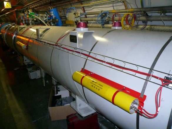
2Fig. 1. An ionization chamber installed on the side of the magnet in the tunnel.
approach to formal verification, and present the formal model and results. Finally, we
reflect on the process, summarising lessons learned and future directions, in Section 5.
2 BLMS Overview
The main purpose of the BLMS is to measure particle loss, and to request beam ex-
traction if the loss level indicates that a quench is likely to occur. The physical principle
underlying particle loss measurement [4, 16] is the detection of energy deposited by sec-
ondary shower particles using specially-designed detectors called ionization chambers
(see Figure 1). There are approximately 4000 ionization chambers strategically placed
on the sides of the magnets all around the LHC tunnel underground. The ionization
chambers produce electrical signals, based on the recording of shower particles, which
are read out by acquisition cards. Acquisition cards, also located in the tunnel and
therefore implemented by radiation-tolerant electronics, acquire and digitize the data
and transmit the digitized data to the surface above the tunnel using optical links. At the
surface, data processing cards named BLETCs receive the data and decide whether or
not the beam should be permitted to be injected or to continue circulating. Each acquisi-
tion card receives data from eight ionization chambers, and each BLETC receives data
from two acquisition cards. A BLETC provides data to the Logging, Post Mortem, and
Collimation systems that drive on-line displays in the control room, perform long-term
storage for offline analysis, and setup the collimators automatically. Due to demanding
performance requirements, BLETCs are implemented on FPGAs, which include the re-
sources needed to implement complex processing and can be reprogrammed making
them ideal for future upgrades or system specification changes.
Figure 2 shows a block diagram of the processes on a BLETC FPGA. In the follow-
ing, we briefly describe each of the four main processing blocks on a BLETC card.
(a) Receive, Check, and Compare (RCC): The RCC block receives data directly
from the acquisition cards, and attempts to detect erroneous transmissions by using
Cyclic Redundancy Check and 8B/10B algorithms [7, 14].
(b) Data Processing: Whether or not a quench results from particle loss depends
on the loss duration and the beam energy. Given the tolerance acceptable for quench
3Data Processing
MAX Values
01 Logging
(Logging)
Data Successive
Receive, Check, and Compare
Combine Running Sums
Post Post
02 Mortem Mortem
Data Successive
Data
Combine Running Sums
from
Tunnel
Collimation
Mux Collimation
Data
16
Data Successive Threshold Beam
Combine Running Sums Comparator Dump
Error & Status
Reporting
Beam Dump Logging Beam Energy
Fig. 2. Block diagram of a BLETC card.
prevention, the quench threshold versus loss duration is approximated by the minimum
number of sliding integration windows (called running sums) fulfilling the tolerance.
In order to achieve the required dynamic range (domain of variation of losses), the
detectors use both Current-to-Frequency converter and Analogue-to-Digital converter
circuitries. The Data Combine block merges these two types of data coming from a
detector so as to send a single value, referred to as a count, to the SRS block. The
implementation of the SRS block is described in Section 3.
(c) Threshold Comparator: Every running sum needs to be compared to the thresh-
old determined by the beam energy reading at that moment. The comparator initiates a
beam dump request if any of the running sums is higher than its corresponding thresh-
old. Beam dump requests are forwarded to the Beam Interlock System which initiates
the beam dump. There are 12 running sums calculated for each 16-detector channel al-
located to a BLETC card. There are 32 levels (0.45 to 7 TeV) of beam energy and each
processing module holds data only for those 16 connected detectors. Thus, a total of
6,144 threshold values need to be held on each card.
(d) Logging, Post Mortem and Collimation: To be able to trace back the loss sig-
nal development, the BLMS stores the loss measurement data. This data is sent to the
Logging and Post-Mortem systems for online viewing and storage. For the purpose of
supervision, the BLMS drives an online event display to show error and status informa-
tion recorded by the tunnel electronics and the RCC process as well as the maximum
loss rates seen by the running sums. Each BLETC card also provides data to the Colli-
mation system for the correct alignment and setup of the collimators.
4subtract
Accumulate
A running sum
A-B ACC
Vn
V1 V2 V3 . . . Vn B
new value
shift register
Fig. 3. Block diagram showing how to produce and maintain a continuous running sum of arriving
values.
3 Successive Running Sums (SRS)
Beam losses can happen at different rates, compared to the number of cycles of the
beams around the tunnel. One-cycle failures are called ultra-fast losses. Multi-cycle
losses can be classified as: very fast losses, which happen in less than 10 ms; fast losses,
which happen between 10 ms and 1 s; and, steady losses, where the beam is lost over
one second or more [12].
Processing the data collected by the detectors involves an analysis of the loss pattern
over time, accounting for the energy of the beam. The processing procedure is based on
the idea that a constantly updated moving window can be maintained in an accumulator
by adding the incoming (newest) value and subtracting the oldest value (see Figure 3).
The number of values in the window is its integration time. Ideally, we would have
an unbounded number of windows with lengths covering the whole spectrum of times
from 40 micro-seconds (the rate at which data from detectors enter a BLETC card)
to 100 seconds, for detecting all losses from ultra-fast up to steady. To approximate
this ideal with finite resources, the BLMS is given the tolerance acceptable for quench
prevention, and the quench threshold versus loss duration curve is approximated by the
minimum number of windows that meet the tolerance.
Long moving windows, that is, windows with large integration times, are required,
which means keeping long histories of received count values. To accomplish this goal
with relatively narrow shift registers, the SRS uses consecutive storage of sums of
counts. Instead of storing all the values needed for a sum, the SRS accumulates many
values as a partial sum, thereby using only a fraction of the otherwise needed mem-
ory space. The partial sums for a window with a large integration time are chosen so
that they also serve as the sums calculated by a window with a smaller intergration
time. This technique works by feeding the sum of one shift register’s contents, every
time its contents become completely updated, to the input of another shift register (see
Figure 4). By cascading shift registers like this, very long moving windows can be con-
structed using a significantly small amount of memory. This scheme is the basis for the
SRS implementation in each BLETC.
The SRS implementation minimizes resource usage by using smaller, previously
calculated, running sums in the calculation of larger, later running sums, which there-
fore do not need extra summation values to be stored. In addition, it makes use of
multipoint shift registers that are configured to give intermediate outputs, referred to
5shift register 1
new value
1 2 3 . . . n
read enable shift register 2
+ 1 2 3 . . . m
shift register 3
read delay
+ 1 2 3 . . . k
read delay
+ ...
Fig. 4. Block diagram showing a configuration for efficient summation of many values.
as taps. The taps provide data outputs at certain points in the shift register chain, thus
contributing to the efficient use of resources.
In the SRS implementation, one shift register’s sum is fed as input to another shift
register. Therefore, the best achievable latency of each shift register is equal to the
refreshing time of its preceding shift register, i.e., the time needed to completely update
its contents. The read delay signal (see Figure 4) of each shift register holds a delay
equal to this latency to ensure correct operation. The delay is equal to the preceding
shift register’s delay multiplied by the number of cells to be used in the sum.
Figure 5 shows the implementation of SRS in a BLETC. It consists of 6 slices,
where each slice computes two running sums (e.g., slice 4 computes running sums RS6
and RS7) with the use of a multipoint shift register, two subtractors and two accumula-
tors (see Figure 6).
As shown in Table 1, cascading 6 slices is enough to reach the approximately 100
second integration limit required by the specifications given by the scientists and engi-
neers who designed the machine protection strategy for the LHC.
4 Verification of the SRS Implementation using HOL4
In this section, we describe our approach to formal verification of the SRS component
of a BLETC, and present the formal model and results.
4.1 Introduction
Our formal verification effort uses mechanised logical deduction, or theorem proving.
In general, theorem proving is used to show that desired properties of a system are
logically implied by a formal model of the system. We use the HOL4 open source
software tool [8, 13], which was developed initially at the University of Cambridge, but
now by an international team. HOL4 enables the construction of theories in Higher-
Order Logic (HOL) [2], a formal logic with a similar expressive power to set theory
that is widely used for formalising hardware and software models and statements about
them. The implementation of HOL4 uses Milner’s LCF approach [6]: a small “kernel”
implementing the primitive rules of the logic, and convenient derived rules and tactics
6Datain 0
1
read enable
shift register
width = 2
tap0 tap1
(1) (2)
0
read enable
1
shift register
width = 16
tap0 tap1
(8) (16)
0
read delay 2 steps
1
shift register
width = 128
tap0 tap1
(32) (128)
0
read delay 64 steps 1
shift register
width = 256
tap0 tap1
(32) (256)
0
read delay 2048 steps 1
shift register
width = 64
tap0 tap1
(16) (64)
0
read delay 16384 steps
1
shift register
width = 128
tap0 tap1
(32) (128)
Fig. 5. Block diagram showing the implementation of SRS in a BLETC.
implemented in terms of the kernel. Every theorem ultimately comes from the kernel,
and this fact provides high assurance of the logical soundness of the verification results
obtained using the system.
HOL4 is an interactive theorem prover: the user provides the high level proof strat-
egy by composing functions that automate common chains of logical deduction. The
work described here could have been done using other systems such as HOL Light [5],
Isabelle/HOL [10], ProofPower [1], PVS [9] or Coq [3]. The first three use essentially
the same higher-order logic as HOL4, whilst PVS and Coq support more powerful
logics. While offering less “push-button” automation than other kinds of formal ver-
ification such as model-checking, machine-assisted theorem proving using HOL4 is
appropriate for verifying the SRS, since it gives a way to very explicitly parameterize
the model.
Our goal is to build a generic model of the SRS structure, and to prove that it sat-
isfies its specification, that it calculates approximate running sums of received count
values within acceptable error margins. Let RS n denote, as in Figure 5, output n of the
SRS structure, which is supposed to compute a sum of received count values, and let
7Slice
shift register
new value
1 2 3 . . m . . n
tap0 tap1
subtract Accumulate
A
A-B ACC running sum X
B
Vn
A
A-B ACC running sum Y
B
Vm
Fig. 6. Block diagram showing the implementation of each slice.
Range Refreshing
40 µs steps ms 40 µs steps ms slice running sum
1 0.04 1 0.04 slice 1 RS0
2 0.08 1 0.04 slice 1 RS1
8 0.32 1 0.04 slice 2 RS2
16 0.64 1 0.04 slice 2 RS3
64 2.56 2 0.08 slice 3 RS4
256 10.24 2 0.08 slice 3 RS5
2048 81.92 64 2.56 slice 4 RS6
16384 655.36 64 2.56 slice 4 RS7
32768 1310.72 2048 81.92 slice 5 RS8
131072 5242.88 2048 81.92 slice 5 RS9
524288 2097.52 16384 655.36 slice 6 RS10
2097152 83886.08 16384 655.36 slice 6 RS11
Table 1. SRS configuration in BLETC.
true sum n denote this sum. The multi-layered structure of the SRS and the read delay
of each shift register result in the outputs being delayed from the true sum values. A
sketch of the desired correctness statement is:
∀n · RS n = true sum n ± acceptable error
Although Figure 5 suggests that the SRS structure has only twelve outputs (i.e., 0 ≤
n ≤ 11), we obtain a more generic result (that is useful in future upgrades of the system)
by interpreting and proving the statement above for all values of n.
To make the above correctness statement more precise, we need to include the no-
tion of time. The count values arrive at the input of the SRS block every 40 micro-
seconds, which we abstract as a single time step in our logical model. We formalize the
input stream as a function of time: D t denotes the input value to the SRS structure
at time t. In addition, the terms in the above statement depend on this stream of input
8counts. With these refinements, the correctness statement becomes:
∀D n t · RS D n t = true sum D n t ± acceptable error
Prior to defining a formal model of the SRS and proving theorems about it, we
developed an informal “whiteboard-level” argument for why the SRS implements its
intended behavior. The essence of this argument relies on four facts which can be es-
tablished from the structure of the SRS and some details about the timing relationship
between layers:
1. The shift register of each slice (except the first) is updated once the shift register of
its previous4 slice is completely updated, that is, when a count value has propagated
down the full length of the previous slice’s shift register.
2. The integration window of a given shift register in a slice (except the first slice)
can be decomposed into a sequence of non-overlapping segments, S1 , S2 , . . . , Sw
(where w is the width of the shift register) each of which is equal to the size of the
integration window of the shift register of the previous slice.
3. After a period of initialization, the values stored in the shift register of a given slice
(except the first) are the w outputs of the previous slice, where w is the width of the
shift register of this slice.
4. After a period of initialization, the output of each slice is always equal to the sum
of the contents of its shift register.
Using Facts 1, 2 and 3 in an inductive argument, we show that each cell of the
shift register of a given slice, after a period of initialization, always contains the sum of
the SRS inputs for one of the non-overlapping consecutive segments that make up the
integration window of this slice. Then using Fact 4 and arithmetic reasoning, we can
show that the output of this slice, after a period of initialization, contains the sum of the
SRS inputs over its integration window.
While the above paragraph gives the appearance of a straightforward argument for
the correctness of the SRS (corresponding roughly to Theorem 1 in Section 4.3), in fact
the argument involves consideration of many details that arise from the formal model
of the SRS presented in the next section. Using a theorem proving tool enables us to
keep track of these details without losing sight of the overall goal.
4.2 Formal Model of SRS
The first step to prove the correctness statement is to build a logical model of the SRS
structure. We model each building block of the SRS structure that holds a count value
– for example, each cell in each shift register – as a function in HOL5 .
Our model is both a simplification and a generalization of the actual structure of
SRS in BLMS in the following sense. We model an unbounded number of slices (rather
than six slices), each with an unbounded number of shift register cells and taps (rather
4
Here, the phrase “previous slice” refers to the slice whose output is used as input to this slice.
5
The acronym HOL refers to higher-order logic rather than the software tool HOL4. We use the
tool to define a function in the logic.
9Function Intended meaning
tap n x The position of tap x of slice n. (The first position is 0.)
input n A pair (n′ , x) indicating that the input to slice n is output x of slice n′ .
delay n The number of time steps between updates of slice n.
source D n m t The value of the cell that is the direct input to cell m of slice n, at time t,
given input stream D.
SR D n m t The value of cell m of slice n, at time t, given input stream D.
output D n x t The output at tap x of slice n, at time t, given input stream D.
RS D n t The value of running sum n at time t, given input stream D.
update time n t A boolean indicating whether t is an update time for slice n.
Table 2. Descriptions of the HOL functions comprising our model of the SRS structure.
than fixed width shift registers and only two taps), simply by letting indices range over
the natural numbers without explicitly giving limits. This parameterization makes the
model more likely to be applicable to future versions of the system, but also fits more
naturally into HOL than would a bounded model. We defined our formal model to be
at a level of abstraction above the details of circuity that implements basic arithmetic
operations. We use natural numbers throughout, rather than, for example, finite words
that would more accurately model count values. This level of abstraction is sufficient
to answer the questions that originally motivated this work. A separate verification ef-
fort can focus on showing that a more realistic model of hardware circuitry accurately
implements natural number arithmetic.
Table 2 lists the HOL functions comprising our model along with their intended
meanings. The arrangement of the slices is described by functions input n and tap n x.
The read delay of a slice is modeled by delay n. Each slice is modeled by three func-
tions: SR D n m t represents the value of each cell of the slice’s shift register,
source D n m t represents the direct input of each cell, and output D n x t rep-
resents the value of the slice’s output at its taps. The function RS D n t models the
running sums and update time n t checks if it is time to refresh the contents of a slice.
We have both RS and output functions, though RS is easily defined in terms of output,
because RS represents an SRS output (indexed by a single number), whereas output
represents an individual slice output (indexed by slice and tap numbers). By separating
RS and output, we allow for designs where some slice outputs are not SRS outputs, but
may still be used internally as inputs to other slices.
The formal definitions of the functions listed in Table 2 are given in Figure 7. The
definition of input when n = 0 or when n > 6 does not change the structure repre-
sented, since slice 0 is a virtual slice and the real SRS has only six slices, so we give
definitions convenient for theorem proving. A similar comment applies to other defini-
tions when n, representing a slice number, is 0, or when x, representing a shift register
position, is greater than 1. We define all excess taps (where x > 1) to be in the same
position as the last tap.
As explained in Section 3, the delay of each slice is equal to the delay of the slice
it receives its input from multiplied by the number of elements in the input slice used
for the sum. For example in Figure 5, delay 4 = delay 3 × tap 3 0 = 2 × 32. The
10definition of the source function states that the source of each cell m in a shift register
is cell m − 1, except for the first cell whose source is the output of the input slice. For
example, source D 4 7 t = SR D 4 6 t and source D 4 0 t = output D 3 0 t.
The output of each slice is computed every time the contents of its shift register are
updated by adding the incoming newest value (specified by source) and subtracting its
oldest value, that is the value in the cell at the tap position. The content of each cell
of a shift register, SR D n m t is also computed at every update time based on the
value of its source. Every definition in Figure 7 is local (only represents a small part of
the SRS structure) and therefore verification against its intended meaning is relatively
straightforward.
Figure 8 shows the definition of a set of additional functions required to prove our
main results. The function delay sum n represents the cumulative delay of the preced-
ing shift registers of a slice. For example, delay sum 4 = delay 3 + delay 1 + delay 0 =
2 + 1 + 1 = 4. The function last update n t returns the latest time not after t at which
slice n updates, and exact D n x t computes the exact sum of consecutive input counts,
without delay, that output D n x t is supposed to approximate.
4.3 Theorems about the Model
Our central result equates the output of a slice to a sum of consecutive input counts.
More precisely, it says that if slice n was just updated, then the output at tap x is equal to
the sum of ((tap n x)+1)×(delay n) input values, starting from the input delay sum n
time steps ago.
Theorem 1. For all values of D, n, and x, the output of slice n > 0 at an update time
t satisfies
((tap n x)+1)×(delay n)−1
(
X 0 t < m + delay sum n
output D n x t =
m=0
D (t − m − delay sum n) otherwise
Proof. The shift register of slice n is updated every delay n time steps. When updated,
the values in its cells are shifted one cell. Therefore6,
SR D n (m + 1) t = SR D n m (t − delay n)
By induction on m, using the above,
SR D n m t = SR D n 0 (t − (m × delay n))
By induction on t, we can show that output D n x t is a sum of values of consecutive
shift register cells,
tap
X nx
output D n x t = SR D n m t
m=0
6
For presentational convenience, here, we do not provide details for the case when t is small
(e.g., when t < m×delay n). For complete theorem statements and the proof script, please re-
fer to https://github.com/xrchz/CERN-LHC-BLMTC-SRS/blob/master/hol/srsScript.sml.
11tap 0 0 = 0 tap 0 x = 0
tap 1 0 = 1 − 1 tap 1 x = 2 − 1
tap 2 0 = 8 − 1 tap 2 x = 16 − 1
tap 3 0 = 32 − 1 tap 3 x = 128 − 1
tap 4 0 = 32 − 1 tap 4 x = 256 − 1
tap 5 0 = 16 − 1 tap 5 x = 64 − 1
tap 6 0 = 32 − 1 tap 6 x = 128 − 1 (where each x > 0)
... tap n x = 0 (where x ≥ 0 and n > 6)
input 0 = (0, 0) input 1 = (0, 0)
input 2 = (0, 0) input 3 = (1, 1)
input 4 = (3, 0) input 5 = (4, 0)
input 6 = (4, 1) input n = (n − 1, 0) (where n > 6)
delay 0 = 1
delay n = delay n′ × ((tap n′ x) + 1)
where (n′ , x) = input n (and n > 0)
source D n 0 t = output D n′ x t where (n′ , x) = input n
source D n m t = SR D n (m − 1) t (where m > 0)
SR D n m 0 = 0
SR D n m t = if update time n t then
source D n m (t − 1)
else SR D n m t (where t > 0)
output D 0 x t = D t
output D n x 0 = 0
output D n x t = if update time n t then
((output D n x (t − 1)) + (source D n 0 (t − 1))) − (SR D n (tap n x) (t − 1))
else output D n x (t − 1) (where n, t > 0)
n
RS D n t = output D 2
+ 1 (n mod 2)
update time n t ⇐⇒ (t mod delay n = 0)
Fig. 7. Definitions of the HOL functions comprising our model of the SRS structure. tap and
input are defined to match Figure 5. Slice 0 is a virtual slice representing the SRS input; this
enables a succinct definition of source.
delay sum 0 = 0
delay sum n = delay n′ + delay sum n′ where (n′ , ) = input n
last update n 0 = 0
last update n t = if update time n t then t
else last update n (t − 1) (where t > 0)
((tap n x)+1)×(delay n)
(
X 0 tCombining the last two results, output D n x t is a sum of consecutive values of the
first shift register cell, SR D n 0. Thus, we can express output D n x t in terms of
output D n′ x′ t, where (n′ , x′ ) = input n, since the source of SR D n 0 is the pre-
vious (input) slice’s output. Finally, by induction on n, we can express output D n x t
as a function of D alone, as required, using the result above for the inductive case. ⊓
⊔
Since the outputs of a slice stay constant between update times for the slice, Theo-
rem 1 suffices to characterize all outputs at all times. Thus, the SRS structure’s outputs
are equal to the exact running sums of the input counts over windows whose sizes de-
pend on the width of the slice’s shift register and position of the taps. However, the sums
are delayed by the total delay across all previous slices (represented by delay sum).
The fact that the SRS calculates exact, but delayed, sums, is captured in the next
theorem, which relates output D n x t to exact D n x at an earlier time.
Theorem 2. For all values of D, n, and x, the output of slice n > 0 at all times t
satisfies
(
0 last update n t + 1 < delay sum n
output D n x t =
exact D n x (last update n t + 1 − delay sum n) otherwise
Proof. The proof follows from Theorem 1, using the definition of exact, and the fact
that output D n x t has the same value as at the last update time. ⊓
⊔
n true
The function sum is easily defined in terms of exact, namely, true sum D n t =
exact D 2 + 1 (n mod 2) t. Since RS is similarly defined in terms of the output,
Theorem 2 establishes a relationship between the values of RS and of true sum.
We call the difference between the RS values and their corresponding true sums,
caused by the delay, the error. To meet the tolerance acceptable for quench preven-
tion, the SRS specification requires a bound on this error. Without restricting the input
stream, the error is unbounded7. However, according to extensive experimental analysis,
the beam loss over time follows some patterns. By formulating some characterization
of the input stream as constraints on D, we can recover a bound on the error. One of
these constraints is a maximum value for the difference between two consecutive input
count values. This “maximum jump size” can be inferred from the highest quench level
thresholds.
Under such a constraint, we have proved the follwoing result bounding the error of
output D n x t compared to exact D n x t.
Theorem 3. For all k and D satisfying |D (t′ + 1) − D t′ | ≤ k at all times, the
following holds for all slices n > 0, tap positions x, and times t:
t > (tap n x + 1) × (delay n) + delay n + delay sum n =⇒
|output D n x t − exact D n x t| ≤ (tap n x + 1) × (delay n) × k×
(delay sum n − 1 + t mod delay n)
7
For any bound, we can construct an input stream that causes the bound to be exceeded by, for
example, having a sequence of zeroes followed by a sequence of count values much higher
than the bound.
13Furthermore, for all k there exists an input stream Dk satisfying |Dk (t′ +1)−Dk t′ | ≤
k for all t′ and
|output Dk n x t − exact Dk n x t| = (tap n x + 1) × (delay n) × k×
(delay sum n − 1 + t mod delay n)
for all n > 0, x, and t > (tap n x + 1) × (delay n) + delay n + delay sum n.
Proof. By applying Theorem 2, we are left with an inequation involving the function
exact specifically between exact D n x t and exact D n x (last update n t + 1 −
delay sum n). Our assumption on t ensures that we are never in the 0 case of either
Theorem 2 or of the definition of exact. The function exact is defined as a sum of
consecutive values of D; we need to bound the difference between one such sum and
another earlier one of the same size. But if at each step the maximum difference is k,
then the total difference is at most k times the distance between the ends of the two
sums, as required. (We use the fact that last update n t = t − t mod delay n.) The
input stream achieving this bound is given by Dk t = k × t. ⊓
⊔
Theorem 3 gives a bound on the error of a running sum at a given time in terms
of the time step, the slice and tap numbers, and the assumed bound on the difference
between consecutive counts. This bound is tight for the conditions we assume, namely
that the time step is sufficiently high and that the difference between consecutive counts
is bounded, in the sense that it is achievable by an input stream satisfying those con-
ditions. To determine whether an error bound is acceptable with respect to the specifi-
cation of SRS, however, it turns out to be more useful to know the relative size of the
error as a fraction of the true sum. According to the specification of SRS, the running
sums should have a maximum 20% relative error ((|RS D n t − true sum D n t| <
20% × (true sum)). We have not yet characterized the relationship between our error
bound at a given time and the true sum at that time.
The proof of Theorem 3 is straightforward when summarized, as above. However,
as for all of our theorems, there are several non-trivial details underlying the high-level
summary provided. For example, proving that the maximum difference between the end
terms in a sum is the maximum difference between consecutive terms multiplied by the
number of terms requires an inductive argument. Our HOL4 proof script for verification
of SRS consists of 750 lines of code. We proved 69 theorems, including 14 definitions.
In addition, we had to prove approximately 30 generic theorems that were added to
HOL4 libraries during this work.
5 Conclusions and Lessons Learned
We have described a case study in which we used HOL4 theorem prover to verify
properties of the SRS structure within the LHC machine protection system. In this case
study, we built a parameterized model of the SRS structure and showed that its behavior
is correct with respect to its specification. It is likely that the configuration of the slices
and shift registers will need to change in the future as the understanding of the LHC and
14its possible weaknesses increases to accommodate more targeted protections. Thus, the
parameterization in our model is crucial to make it applicable to the future upgrades.
One of our main challenges in this effort was building the formal model and formu-
lating the correctness statements. There are three different sources of complexity that
are inherent in understanding why the SRS structure implements its intended behavior:
(a) the structure of the SRS: although it features considerable regularity, it includes ex-
ceptions to this regularity that complicate reasoning, e.g., the input of one slice may not
be the output of the immediately previous slice, but may be the first or second output
of any earlier slice or even the global input; (b) the non-trivial timing relationships be-
tween different elements of the SRS; e.g., the frequency of updates to the contents of a
shift register depends on the position of the shift register in the layered structure of the
SRS; (c) arithmetic relationships that are not always intuitively apparent at first glance.
While each of these sources of complexity is manageable on its own, reasoning about
the correctness of the SRS is a matter of grappling with all three sources of complexity
at once.
To understand the structure of the SRS, we started with a model of a simplified
structure, which had a more regular arrangement of the slices and ignored the middle
taps, and proceeded to a model which is closer to the SRS implementation in BLMS.
In addition, we used a basic spreadsheet simulation model for a few slices for sanity
testing the correctness formulae. However, some sanity tests related to Theorem 1 led
us astray when we did not know the correct formula for that theorem. The formulae
we conjectured worked for small values of n, and simulating large values of n was
expensive, but the counterexamples were only to be found at large values of n.
The use of mechanized theorem proving to verify the correctness of the SRS be-
havior complements an intensive verification effort based on simulation performed at
CERN. This effort targeted the validity of the SRS as an accurate and fast enough
method by analyzing its behavior (a) in the boundaries of the threshold limits and (b)
in expected types of beam losses, e.g., fast and steady losses. Its results showed that the
current implementation of the SRS, given in Figure 5, satisfies the specification, that is,
the running sums have a maximum 20% relative error.
By contrast, the results in this paper apply to all possible input streams, not just the
sample inputs considered at CERN – our main contribution, as stated in Theorem 2,
showed that the behavior of the SRS is correct for all possible input streams. However,
we do not know if the constraint on input stream given in Theorem 3 is sufficient to
satisfy the maximum 20% relative error bound. One of the potential reasons for this
problem is not knowing how to characterize the input stream to the SRS. Due to the
physical nature of this problem, such a characterization of the input stream is not triv-
ial. While testing and simulation of the SRS on a limited set of input streams offers a
level of confidence that the behavior of SRS satisfies this particular specification, con-
structing a formal proof for all possible behaviors requires a better understanding of
the characteristics of the input stream. One future research direction is to investigate
whether constructing such a formal proof is feasible for the SRS component of BLMS.
Another future research direction is to refine our formal model to a lower level of
abstraction, closer to the hardware level (e.g., by representing count values as finite
words instead of natural numbers). We are also considering verifying a model extracted
15from the Hardware Description Language (HDL) used to synthesize the BLETC FPGA.
Acknowledgment: The authors thank Mike Gordon at the University of Cambridge
for his insightful and helpful feedback during the course of this work.
References
1. R. Arthan. ProofPower manuals. http://lemma-one.com/ProofPower/index/index.html,
2004.
2. A. Church. A Formulation of the Simple Theory of Types. J. Symb. Log., 5(2):56–68, 1940.
3. T. Coquand and G. Huet. Coq manuals. http://coq.inria.fr, 2010.
4. B. Dehning. “Beam loss monitoring system for machine protection”. In Proceedings of
DIPAC, pages 117–121, 2005.
5. J. Harrison. HOL Light manuals. http://www.cl.cam.ac.uk/˜jrh13/hol-light, 2010.
6. R. Milner. “Logic for Computable Functions: Description of a Machine Implementation”.
Technical report, Stanford, CA, USA, 1972.
7. R. Nair, G. Ryan, and F. Farzaneh. “A Symbol Based Algorithm for Hardware Implementa-
tion of Cyclic Redundancy Check (CRC)”. VHDL International User’s Forum, 0:82, 1997.
8. M. Norrish and K. Slind. HOL4 manuals. http://hol.sourceforge.net, 1998.
9. S. Owre, N. Shankar, J. Rushby, and D. Stringer-Calvert. PVS manuals. http://pvs.csl.
sri.com, 2010.
10. L. Paulson, T. Nipkow, and M. Wenzel. Isabelle manuals. http://www.cl.cam.ac.uk/
research/hvg/Isabelle/index.html, 2009.
11. J. Rushby. “Formal Methods and the Certification of Critical systems”. CSL Technical
Report 93-7, SRI International, December 1993.
12. R. Schmidt, R. W. Assmann, H. Burkhardt, E. Carlier, B. Dehning, B. Goddard, J. B. Jean-
neret, V. Kain, B. Puccio, and J. Wenninger. “Beam Loss Scenarios and Strategies for Ma-
chine Protection at the LHC”. In Proceedings of HALO, pages 184–187, 2003.
13. K. Slind and M. Norrish. “A Brief Overview of HOL4”. In TPHOLs, volume 5170 of LNCS,
pages 28–32, 2008.
14. A. X. Widmer and P. A. Franaszek. “A DC-balanced, partitioned-block, 8B/10B transmission
code”. IBM J. Res. Dev., 27:440–451, September 1983.
15. C. Zamantzas. “The Real-Time Data Analysis and Decision System for Particle Flux Detec-
tion in the LHC Accelerator at CERN”. Ph.D. Thesis, Brunel University, 2006.
16. C. Zamantzas, B. Dehning, E. Effinger, J. Emery, and G. Ferioli. “An FPGA Based Imple-
mentation for Real-Time Processing of the LHC Beam Loss Monitoring System’s Data”. In
IEEE Nuclear Science Symposium Conference Record, pages 950–954, 2006.
16You can also read