Robustness of prediction for extreme adaptive optics systems under various observing conditions
←
→
Page content transcription
If your browser does not render page correctly, please read the page content below
A&A 636, A81 (2020)
https://doi.org/10.1051/0004-6361/201937076                                                                         Astronomy
c ESO 2020                                                                                                           &
                                                                                                                    Astrophysics

    Robustness of prediction for extreme adaptive optics systems
               under various observing conditions
                         An analysis using VLT/SPHERE adaptive optics data
                                   M. A. M. van Kooten1 , N. Doelman1,2 , and M. Kenworthy1

      1
          Leiden Observatory, Leiden University, Niels Bohrweg 2, 2333 CA Leiden, The Netherlands
          e-mail: vkooten@strw.leidenuniv.nl
      2
          TNO, Stieltjesweg 1, 2628 CK Delft, The Netherlands

     Received 7 November 2019 / Accepted 4 March 2020

                                                                 ABSTRACT

     Context. For high-contrast imaging systems, such as VLT/SPHERE, the performance of the system at small angular separations is
     contaminated by the wind-driven halo in the science image. This halo is a result of the servo-lag error in the adaptive optics (AO)
     system due to the finite time between measuring the wavefront phase and applying the phase correction. One approach to mitigating
     the servo-lag error is predictive control.
     Aims. We aim to estimate and understand the potential on-sky performance that linear data-driven prediction would provide for
     VLT/SPHERE under various turbulence conditions.
     Methods. We used a linear minimum mean square error predictor and applied it to 27 different AO telemetry data sets from
     VLT/SPHERE taken over many nights under various turbulence conditions. We evaluated the performance of the predictor using
     residual wavefront phase variance as a performance metric.
     Results. We show that prediction always results in a reduction in the temporal wavefront phase variance compared to the current
     VLT/SPHERE AO performance. We find an average improvement factor of 5.1 in phase variance for prediction compared to the
     VLT/SPHERE residuals. When comparing to an idealised VLT/SPHERE, we find an improvement factor of 2.0. Under our 27 dif-
     ferent cases, we find the predictor results in a smaller spread of the residual temporal phase variance. Finally, we show there is no
     benefit to including spatial information in the predictor in contrast to what might have been expected from the frozen flow hypothesis.
     A purely temporal predictor is best suited for AO on VLT/SPHERE.
     Conclusions. Linear prediction leads to a significant reduction in phase variance for VLT/SPHERE under a variety of observing
     conditions and reduces the servo-lag error. Furthermore, prediction improves the reliability of the AO system performance, making it
     less sensitive to different conditions.
     Key words. instrumentation: adaptive optics – methods: numerical

1. Introduction                                                           (WDH) that dominates the wavefront error at small angular sep-
                                                                          arations. The WDH is a manifestation of the servo-lag error
In the search for new exoplanets and earth analogs, dedicated             and appears as a butterfly pattern in the coronagraphic/science
high-contrast imaging (HCI) systems have allowed the angu-                images (see Cantalloube et al. 2018, for details on the WDH).
lar separation of host stars from their surroundings to reveal            The servo-lag error is due to the finite time between the mea-
circumstellar disks and exoplanets. The combination of extreme            surement of the incoming wavefront aberration (caused by atmo-
adaptive optics (XAO) to provide high spatial resolution, coro-           spheric turbulence) and the subsequent applied correction. The
nagraphs to suppress the host star’s light, and data reduction            resulting wavefront error is due to the outdated disturbance
techniques to remove residual effects, allows HCI systems to              information and the closed-loop stability constraints. Owing to
reach post-processed contrasts of 10−6 at spatial separations of          this, the halo is aligned with the dominant wind direction and
200 milliarcseconds (Zurlo et al. 2016). VLT/SPHERE is a HCI              severely limits the contrast at small angular separations even
system that has discovered two confirmed planets: HIP 65426b              after post-processing techniques. The servo-lag error prevents
(Chauvin et al. 2017) and PDS 70b (Keppler et al. 2018). It has           VLT/SPHERE from achieving its optimal performance when
also discovered a vast array of debris, protoplanetary, and cir-          coherence times are below 5 ms (Milli et al. 2017).
cumstellar disks (e.g., Avenhaus et al. 2018; Sissa et al. 2018).             The XAO system, SAXO, has a temporal delay of approx-
Operating with a tip/tilt deformable mirror (TTDM), a 41-by-41            imately 2.2 SHWFS camera frames. The HODM is controlled
high order deformable mirror (HODM), and a Shack-Hartmann                 using an integrator with modal gain optimisation (Petit et al.
wavefront sensor (SHWFS) sampling at 1380 Hz, the XAO sys-                2014). Within this framework, one solution to minimise the
tem of VLT/SPHERE, SAXO delivers Strehl ratios greater than               delay in SAXO itself is to run everything faster. However, this
90% in the H band (Beuzit et al. 2019).                                   solution poses a number of hardware challenges with a new
    A major challenge with VLT/SPHERE (and other HCI sys-                 HODM that can run at the desired speed, a wavefront sensor cam-
tems to varying degrees) is the presence of the wind-driven halo          era with fast readout, and a more powerful real-time-computer.

                                                      Article published by EDP Sciences                                          A81, page 1 of 9
A&A 636, A81 (2020)
One alternative solution is to upgrade the controller with a control
scheme that predicts the evolution of the wavefront error over the
time delay. In this paper, we look at the potential of prediction to
improve the performance of SAXO especially when the servo-lag
error is the dominant residual wavefront error source (i.e., small
coherence times).
Many different groups have worked on predictive control as
a means of improving the performance of an adaptive optics
(AO) system by minimising the servo-lag error. We highlight a
few results from the last 15 years. Prediction, within the con-
text of optimal control, is an ingredient in finding the optimal
controller. Linear quadratic Gaussian (LQG) control has been
explored by Petit et al. (2008) for general AO systems to perform
Fig. 1. Kernel density functions for the seeing, coherence time, tur-
vibration filtering with the Kalman filter. On-sky demonstrations bulence velocity, and guide star magnitude (r band) showing the con-
of the LQG controller for tip-tilt/vibrational control are provided ditions under which the VLT/SPHERE telemetry was taken. The first
in Sivo et al. (2014). Laboratory work to include higher order three panels are measurements closest to the time of the observation out-
modes for atmospheric turbulence compensation (Le Roux et al. put by the MASS-DIMM (accessed via ESO Paranal query form). The
2004) has demonstrated a reduction in the temporal error show- corresponding targets were found at the VLT/SPHERE ESO archive and
ing predictive capabilities. The H2 optimal controller (closely their r-band magnitudes were found in the VizieR catalog. The ker-
related to LQG) has been tested on-sky (Doelman et al. 2011) nel density functions are a nonparametric estimation of the probability
showing a reduction in the temporal error for tip-tilt control. functions.
For multi-conjugate AO systems, a temporal aspect to the phase
reconstruction for each layer has been implemented; the spatial- conditions. Previous work on prediction in the AO community
angular predictor is formed by exploiting frozen flow hypothesis has focused on one or two case(s) on-sky for demonstrations
and making use of minimum mean square error estimator (with of prediction, successfully showing the feasibility of predictive
analytical expressions for the stochastic process) (Jackson et al. control. We look at how a linear minimum mean square error
2015). (LMMSE) predictor performs a posteriori on VLT/SPHERE AO
Within the HCI community, there have been many efforts to telemetry data under a large set of various observing conditions
incorporate prediction into the AO control algorithm. Building (such as guide star magnitude, coherence time, and seeing con-
on Poyneer & Macintosh (2006), predictive Fourier control, pro- ditions).
posed in Poyneer et al. (2007), makes use of Fourier decompo- We organise this paper as follows: we introduce and sum-
sition and the closed-loop power spectral density (PSD) to find marise our SAXO data set in Sect. 2. In Sect. 3 we out-
components due to frozen flow. Using Kalman filtering a pre- line our methodology, including the structure of our predictor
dictive control law is determined resulting in a reduction of the (Sect. 3.1). We elaborate on how we apply the predictor to the
servo-lag error. Other efforts in HCI have focused on splitting VLT/SPHERE SAXO telemetry data and we present our results
the prediction step from the controller. This is done by first esti- in Sect. 4, discussing them in Sect. 5. We look at how the predic-
mating the pseudo-open loop phase (slopes, or modes), apply- tor performs under different conditions as well as the stationarity
ing a prediction filter, and then controlling the HODM using of the turbulence. The implications of the results are discussed
the predicted phases as input into the controller. This approach in Sect. 5.4, concluding in Sect. 6 including future research
allows for a system architecture that can turn prediction on directions.
and off without affecting the control loop. A similar structure
has been implemented using the CACAO real-time computer
(Guyon et al. 2018). Empirical orthogonal functions (EOF) is a 2. SAXO data
data-driven predictor that aims to minimise the phase variance.
Implemented on SCExAO (an HCI instrument at the Subaru tele- The SAXO system has the option to save the full (or partial)
scope using the CACAO real-time computer) it has been demon- XAO telemetry, including HODM positions, SHWFS slopes,
strated (Guyon et al. 2018) that EOF improves the standard SHWFS intensities, interaction matrix, at the discretion of the
deviation of the point-spread-function over a set of images. How- instrument user. In this paper, we make use of 27 SAXO data
ever, the improvement is less than expected from initial simu- sets taken between 2016 and 2019. By limiting ourselves to
lations (Guyon & Males 2017). Similar methods minimise the these years we also have estimations of the atmospheric condi-
same cost function as EOF but with a different evaluation of tions (seeing, coherence time, and turbulence velocity) from the
the necessary covariance functions (see Sect. 3.1) as reported MASS-DIMM instrument located approximately 100 m away
in van Kooten et al. (2019) and Jensen-Clem et al. (2019). Cur- from UT4. The conditions under which our data were acquired
rent a posteriori tests, using AO telemetry (Jensen-Clem et al. are summarised in Fig. 1, where we plot the kernel den-
2019), show an average factor of 2.6 improvement for con- sity functions estimated from the data. We note that the data
trast for separations from 0 to 10 λ/D. This approach to pre- set is biased toward shorter coherence times (tau), where the
diction will be implemented at the Keck telescope. One benefit median coherence time are 2.5 ms; from Milli et al. (2017) and
to separating the prediction and the control steps is that the Cantalloube et al. (2018) we expect the WDH to be dominant
behaviour of the input disturbance (atmospheric induced phase (and thereby the servo-lag error) when the coherence time drops
fluctuations) can be studied for a given system and telescope below 5 ms. For completeness, the data set has a couple of data
site location, along with tests performed with AO telemetry sets with longer coherence times. The turbulence velocity is the
data. We take this approach in this work, building on our earlier velocity of the characteristic turbulent layer as determined by the
work (van Kooten et al. 2019), looking solely at the predictabil- MASS-DIMM instrument and is associated with a characteristic
ity of the pseudo open-loop slopes under various atmospheric altitude determined from the atmospheric profile. Therefore, it
A81, page 2 of 9M. A. M. van Kooten et al.: Robustness of prediction for extreme adaptive optics systems under various observing conditions
(2005), Kasper (2012), and Cantalloube et al. (2018), we see that
minimising the lag results in an improvement in contrast but ulti-
mately also depends on the coronagraph of choice and how it
interacts with the residual phase at small angular separations. We
also do not have focal plane images taken at the same time as the
data sets, making a clear claim of improvement unreliable. The
metric we adopt is the temporally and spatially averaged wave-
front phase variance.
3.1. LMMSE prediction
For our predictor we chose a data-driven method called the
LMMSE predictor. This approach provides a flexible frame-
work that allows us to implement the predictor in three different
ways: batch, recursive, and with an exponential forgetting factor
(van Kooten et al. 2019).
A single point i of a phase screen at time t is given by yi (t),
while u(t) is a P2 ×1 column vector containing a collection of
Fig. 2. Power spectral densities, estimated using the Welch method, for
all the data sets; both for the full VLT/SPHERE estimated pseudo open- P2 phase values on a discrete spatial grid at time t. We assume
loop phases and for the reconstructed VLT/SPHERE residual phases. that the future value of a given phase point, ŷi at the discrete
time index t + d, is a linear combination of the most recent phase
does not necessarily indicate the speed of the jet stream layer values at time t. The predictor coefficients are denoted as ai . The
but provides a tracer atmosphere velocity. For most of the data cost function of our predictor, with t as the time average oper-
we have bright guide star magnitudes with a mean of 5 mag in ator, is then
the r band (the wavefront sensor bandwidth), resulting in high
min ai h||yi (t + d) − aTi w(t)||2 it , (1)
signal-to-noise ratios (S/N) for the SHWFS in all cases. The see-
ing has a Gaussian-like distribution with a mean of 1.3 arcsec. A where w(t) includes a set of Q most recent measurements,
full summary of the entire data set (including time of observa-
tion) is provided in Table A.1. Each of the 27 data sets differ in T
length and range from 10 s to 60 s, allowing us to probe differ- w(t) = u(t)T u(t − 1)T u(t − 2)T ... u(t − Q)T . (2)
ent conditions while still having the opportunity to observe the
behaviour of turbulence on timescales of a minute. We allowed for both spatial and temporal regressors gathered
To study the influence of prediction on our data sets, we into w(t) – a P2 Q × 1 vector. We denoted predictors of various
estimated the pseudo-open loop phases, thereby applying pre- orders by indicating the spatial order P (spatially limiting our-
diction to the zonal two-dimensional grid of phase values and selves to a box of order P, symmetric around the phase point of
not the modes. We performed the open-loop estimation using the interest, resulting in P2 spatial regressors) followed by the tem-
HODM commands only because SAXO saves the full HODM poral order Q; for example, a “s5t2” predictor has P = 5 and
voltages, not just the updates (see Appendix B). We converted Q = 2.
to phase using the laboratory measured HODM influence func- Solving Eq. (1) for our zero-mean stochastic process, the
tions. As a result, we neglected the spatial frequencies beyond solution can be written in terms of the inverse of the auto-
the spatial bandwidth of the HODM and therefore underesti- covariance matrix and cross-covariance vector (Haykin 2002)
mated the open-loop phase at higher spatial frequencies. We took
ai = C+ww cwyi , (3)
this approach after first considering the more traditional method
of using the wavefront sensor measurements and unravelling the where + denotes a pseudo inverse; Cww is the auto-covariance
pseudo open-loop phase from the SHWFS measurements and matrix of w, the vector containing the regressors; and cwyi is the
knowledge of the controller state. Without full knowledge of the vector containing the cross-covariance between the true phase
modal gains and controller at each time step, as in our case, this value, yi and w.
method provides an inaccurate estimation. We can estimate the covariances in Eq. (3) directly from a
In Fig. 2, we plot the resulting PSDs for the final pseudo training set, forming a fixed batch solution. Alternatively, we can
open-loop phase from the VLT/SPHERE telemetry (SPHERE form a recursive solution making use of the Sherman-Morrison
full) and the closed-loop phase of VLT/SPHERE residuals and formula (a special case of the Woodbury matrix inversion
identify some key features. There are peaks around 40 Hz and lemma). In Eq. (4) through to Eq. (6) we inserted the expo-
60 Hz in both the open and closed-loop PSDs. Performing nential forgetting factor in the update in the following equations,
a modal analysis we find that the peaks appear for Zernike thereby forming our final LMMSE implementation. The recur-
modes 7−11 (Noll indexing; Noll 1976) with varying ampli- sive form is given in Eqs. (4) and (5) with λ = 1, such that all
tudes. The second feature is the increase in power at high tem- previous data is weighted equally, as follows:
poral frequencies for the closed-loop PSD (i.e., the so-called
waterbed effect, a result of Bode’s sensitivity integral). cwyi (t − d) = λcwyi (t − d − 1) + w(t − d)yi (t − d) (4)
C+ww (t − d) = λ −1
C+ww (t − d − 1) − k(t − d) (5)
3. Methodology
with
Although we are ultimately interested in the improvement in
contrast using prediction, we limit ourselves in this work to λ−2 C+ww (t − d − 1)w(t − d)wT (t − d)C+ww (t − d − 1)
studying the minimisation of the servo-lag error. From Guyon k(t − d) = · (6)
1 + λ−1 wT (t − d)C+ww (t − d − 1)w(t − d)
A81, page 3 of 9A&A 636, A81 (2020)
By updating Eqs. (4) and (5), the coefficients can be found for 4. Results
each time step using Eq. (3). The recursive solution goes on-line
immediately with the initial auto-covariance being set to diag- We find that prediction provides a reduction in averaged phase
onal matrices with large values (as done with recursive least- variance when compared to the VLT/SPHERE SAXO residuals.
squares methods) and the cross-covariance vector set to ones. An example of how prediction behaves spatially and temporally
By adjusting the forgetting factor, we can weigh old data by less for a slice across the telescope aperture is shown in the bottom
compared to the most recent measurements, therefore allowing panel of Fig. 4. We see a reduction in the phase compared to
the tracking of slowly varying signals. the VLT/SPHERE residuals and see a more uniform solution in
time and space. In Fig. 5 we summarise the results of running
prediction on all of our data sets. As mentioned above, the aver-
3.2. Comparison with EOF aged phase variance is found by using the last 5 s of the data.
The data sets all vary in length. When we see a reduction in
Methods such as LMMSE and EOF (see Guyon & Males 2017) the residual phase variance, we would expect an improvement
and similar techniques (see Jensen-Clem et al. 2019) all min- of performance for the XAO system for all cases independent
imise the same cost function, but the evaluation of Eq. (3) is of the guide star magnitude, the seeing, and the coherence time.
different in each case; we note that the cost function is slightly We observe a reduction in the spread of residual phase variance,
different when including exponential forgetting factor. In EOF, with prediction providing a more uniform performance for var-
the solution is estimated with the inverse of the auto-covariance ious conditions; see the kernel density function plots in the top
determined using a singular-value-decomposition that is re- panel of Fig. 5.
estimated on minute timescales. The amount of data used to In Fig. 6 we plot the ratio of the recursive s1t10 predic-
estimate the prediction filter, the numerical robustness, the noise tor residual phase variance to the VLT/SPHERE residual phase
properties of the system, and the atmospheric turbulence above variance defining this as the “ratio of improvement” as a func-
the telescope all contribute to the performance of these algo- tion of coherence time. In the same figure, we add the ratio of
rithms and the final computational load. Therefore one imple- improvement for the same recursive s1t10 predictor and an ide-
mentation might be more suited for specific conditions than the alised VLT/SPHERE integrator (batch s1t1) against coherence
other, but the three methods can, in ideal conditions, result in the time. We calculate the average ratio of improvement to be 5.1
same performance. and 2.0, respectively. Figure 6 shows the relative seeing condi-
tions indicated by the size of the marker; smaller marker sizes
3.3. Applying prediction to SAXO telemetry indicate better seeing conditions.
We evaluate several predictors, varying both spatial and tem-
From the estimated open-loop phases (which results in a 240- poral orders. We find that there is no gain in performance by
by-240 phase screen using the HODM modes) we bin the data adding spatial regressors and find that temporal regressors per-
to 60-by-60 phase screens for computational memory purposes. form equally as well. These results are summarised in Table 1.
We then performed prediction on the estimated open-loop phases We see minimal evidence of nonstationary behaviour of
assuming a 2-frame delay. For each phase point, we estimated optical turbulence. First, by looking at the coherence times in
a unique set of prediction coefficients using the equations as Table A.1, we do not see significant change in coherence time for
outlined in Sect. 3.1. Our aim is to focus on the prediction data taken on the same night – showing that on 100 s time scales
capabilities, ignoring the control aspect by assuming a perfect the statistics of optical turbulence do not vary significantly. Sec-
system – no wavefront sensor noise and a HODM that can per- ond, on shorter timescales, we do not see evidence of nonsta-
fectly correct all spatial frequencies predicted – and only includ- tionary turbulence. In Fig. 3, we plot the batch, recursive, and the
ing the delay. We note that this results in no fitting error, no forgetting LMMSE for a s1t10 predictor. From the average resid-
spatial bandwidth limitations, and no temporal bandwidth lim- ual phase variances, we see that the batch and recursive perform
itations on the achievable performance. the same over the full 40 s period. We do see a slight improve-
We ran batch, recursive, and forgetting (with λ = 0.998 as ment for the forgetting LMMSE, implying a slight time-variant
this value gives the best performance assuming λ , 1) LMMSE behaviour of the pseudo open-loop phase but nothing significant.
predictors for each prediction order. We then subtracted the pre-
dicted phase from the pseudo open-loop phase 2 frames later
resulting in the residual predictor phase. From the phases we 5. Discussion
calculated the averaged phase variance by taking the final 5 s
5.1. Comparison of the prediction residuals to the
of the data set, and therefore, all the different predictors have
VLT/SPHERE residuals
converged; we calculated the spatio-temporally averaged phase
variance. We started with the performance of a s1t1 predictor. We should note the difficulties in performing a direct compar-
The s1t1 is a zero-order predictor because it only makes use of ison between the predictor residuals to the real VLT/SPHERE
the most recent measurement for that given phase point, mak- residuals. There are a few challenges, with the first being a dif-
ing it analogous to an optimised integrator (with a gain close ference in delay. In our estimation of the open-loop phase we
to unity) in our simulations; we refer to the s1t1 as the ideal choose to round the frame delay to a whole frame; therefore our
VLT/SPHERE performance. predictor sees a delay of 2 frames (or 1.45 ms) while the real
We performed simulations testing a variety of predictors system delay, and thereby encoded in the real VLT/SPHERE
with different spatial and temporal orders including s1t3, s1t10, residuals, is 2.2 frames (1.59 ms). We therefore assume that the
s3t1, and s3t3. We looked at how the three different imple- VLT/SPHERE residuals immediately have a larger phase vari-
mentations of the LMMSE for each prediction order behave ance compared to the case where the true delay is 2 frames.
(see Fig. 3). In Sect. 4 we present the results for the recursive An alternative option to rounding the delay frames is to inter-
s1t10 predictor, which performs the best out of all the different polate, which is a step that would have also introduced an error.
orders. We make use of the HODM commands which are saved as the
A81, page 4 of 9M. A. M. van Kooten et al.: Robustness of prediction for extreme adaptive optics systems under various observing conditions
Fig. 3. Top panel: time series showing the estimated pseudo open-loop in black, compared with the VLT/SPHERE residual in blue for a random
SAXO telemetry data set. Other plots (all with the same y-scale): various predictor residual phase variances (various green and purple lines)
compared to the VLT/SPHERE residuals for the same data. The averaged phase variance, in µm2 , for the last 5 s is indicated in the top right corner
of each plot. The forgetting s1t10 (abbrev. for) does not perform significantly better than the recursive s1t10 (abbrev. rec). Secondly, the s3t3 does
not perform better than the s1t10.
total voltage on the HODM, not the update to the HODM. The conditions (see Figs. 6 and 7). We briefly discuss the behaviour
SHWFS, however, is used to determine the real VLT/SPHERE for various observing parameters including coherence times,
residuals and therefore see higher order spatial frequencies, turbulence velocity, seeing, and finally guide star magnitudes.
potentially increasing the residuals if this was not the case. Per- Looking closely at Fig. 6 and the behaviour for various
haps the most substantial contribution to the final performance coherence times we do not find any correlation between the
of VLT/SPHERE results from the fact that the VLT/SPHERE coherence time and performance for the true VLT/SPHERE
performance will be limited by operational parameters. The residuals. However, when looking at the idealised VLT/SPHERE
controller will need to be stable and robust on-sky, potentially behaviour we see, at smaller coherence times, an exponential-
resulting in a loss of performance when compared to our ide- like gain in the ratio of improvement in which the asymptote is
alised situation. Therefore, in Figs. 5 and 6 we plot the idealised the Nyquist sampling frequency (2/WFSf = 2/1380 = 1.45 ms).
VLT/SPHERE (batch s1t1) as well as the VLT/SPHERE resid- This behaviour for the idealised case is as expected, where we
uals. The true gain in prediction will be between the idealised have a larger improvements for shorter coherence times. We then
VLT/SPHERE and real VLT/SPHERE residuals and the ratio of look at the relation between the ratio of improvement and tur-
improvement will fall between 5.1 and 2.0. bulence velocity (middle plot of Fig. 7). We expect a similar
behaviour to that of the coherence time as they are related. We
5.2. Performance under different conditions note that we also see no correlation for the ground layer wind
speeds measured by the nearby meteorological tower. Studying
Our data set and analysis is unique, showing that with prediction, the relation between the seeing and the ratio of improvement we
there will be an improvement under almost all conditions even notice an asymptotic behaviour where the ratio improves for bet-
for long coherence times, and no loss in performance with pre- ter seeing conditions. We do not see any dependence between
diction is observed. However, the data set does not show any clear performance and S/N (or guide star magnitudes; left plot of
correlations between predictor performance and observational Fig. 7). For the VLT/SPHERE residuals, the lack of correlation
A81, page 5 of 9A&A 636, A81 (2020)
Fig. 4. Vertical slice across the telescope aperture (y-axis) showing the wavefront phase in µm (indicated by the colour-bars), plotted as a function
of time for the pseudo open-loop phase (top), the VLT/SPHERE residual phase (middle), and s1t10 predictor residual phase (bottom) for the same
night as Fig. 3. Comparing the bottom two panels (colour map is the same in both), we can see the prediction residuals have a flatter and more
uniform appearance compared to the real VLT/SPHERE residuals.
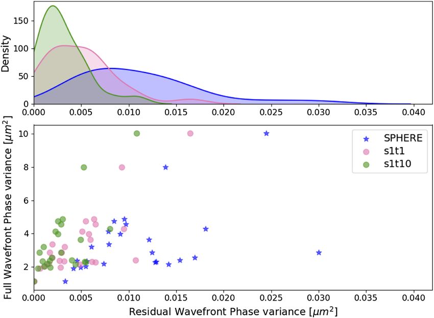
Fig. 5. Top: Kernel density function estima-
tion for the averaged phase variances plotted
in the bottom plot. The change in spread of
the values is shown. Bottom: pseudo open-loop
averaged wavefront phase variance compared to
residual averaged wavefront phase variance for
VLT/SPHERE, a batch s1t1 (i.e., idealised inte-
grator for VLT/SPHERE), and a recursive s1t10
predictor. The points move from right to left, indi-
cating that a s1t1 does better than VLT/SPHERE
and a high order predictor does even better than
the s1t1.
between performance and S/N is as expected from laboratory ages do not reflect the exact values at the time of observation.
and on-sky validation of SAXO by Fusco et al. (2016) at these Alternatively, the behaviour of the SAXO controller is limited
guide star magnitudes. We also note that for long coherence by internal system requirements (such as vibration rejection) and
times VLT/SPHERE is often looking at fainter targets since the not the observing conditions, resulting in a lack of correlation
conditions are ideal. This is the case for our data as well (see between observing conditions and gain in performance.
Table A.1). In summary, we see a relation between the true Studying Fig. 6, we can see that the ratio of improvement
VLT/SPHERE residuals and the seeing, but for the idealised when using idealised VLT/SPHERE as a benchmark behaves
VLT/SPHERE case we see a relation between the improve- very differently than the true VLT/SPHERE case. For a direct
ment and the coherence time, as expected. The lack of corre- comparison to VLT/SPHERE, we do not see any correlations
lation between ratio of improvement and the other observing between the ratio of improvement and the coherence time. How-
parameters could be a result of the different locations of ever, for the idealised case, we see that at longer coherence times
VLT/SPHERE and MASS-DIMM (which measures the observ- we have no improvement since the SAXO XAO system can
ing parameters) and that the values determined over minute aver- already perform well.
A81, page 6 of 9M. A. M. van Kooten et al.: Robustness of prediction for extreme adaptive optics systems under various observing conditions
Fig. 6. Ratio of improvement, found by tak-
ing the ratio of an idealised integrator on
VLT/SPHERE to a recursive spatial-temporal
predictor (s1t10) phase variance as calculated
from the last 5 s of data, as a function of coher-
ence time. The size of the markers indicates the
MASS-DIMM seeing conditions at the time of
observation. The average ratio of improvement
is 5.1 when comparing the prediction to the
real VLT/SPHERE residuals. When looking at
the idealised VLT/SPHERE, we find an aver-
age ratio of improvement of 2.0 in wavefront
variance reduction.
Table 1. Averaged phase variance for the pseudo open-loop, VLT/SPHERE residuals, s1t3 residuals, s3t3 residuals, and the s3t1 residuals.
Time of data Pseudo open-loop [µm2 ] VLT/SPHERE [µm2 ] s1t3 [µm2 ] s3t3 [µm2 ] s3t1 [µm2 ]
2017-07-19T22:54:55.000 1.963 0.005 0.002 0.002 0.002
2017-07-19T23:16:39.000 2.856 0.012 0.001 0.001 0.002
2017-07-19T23:22:02.000 2.400 0.015 0.004 0.004 0.011
2017-07-19T23:50:33.000 2.148 0.014 0.004 0.004 0.005
Notes. Comparing the last three columns, there is no gain by including spatial regressors to the prediction algorithm and the s1t3 does better than
the s3t3.
5.3. Time-invariant turbulence statistics improvement is one, indicating no gain but also, notably, no loss
Observing the behaviour of the three (batch, recursive, and expo- in performance.
nential forgetting) implementations of the LMMSE, we can A more notable result is from the kernel density functions
comment on the stationarity of the turbulence. The LMMSE plotted in the top panel of Fig. 5. The spread of the averaged
finds the optimal prediction coefficients determined from the phase variance is less for the s1t10 predictor, indicating a more
training set. The batch is trained on the first 5 s and the recur- uniform performance in phase variance reduction for differ-
sive trains continuously. We note the residual phase variances for ent observing conditions. From an observational point of view,
the last 5 s for each case; we do not see a significant difference having a more stable correction under different conditions is
between the batch and recursive solutions in any case, indicating desirable, especially for the cases on surveys in which observers
the statistics of the turbulence has not changed over the mea- might be targeting similar objects and can perform reference star
surement period. Studying the recursive solution, we look at the differential imaging from a library.
behaviour of the prediction coefficients in time across the aper- The ratio of improvement we find is 5.1, but this is probably
ture. We do not see any notable changes over the entire period an overestimate of the improvement we could achieve on-sky.
once the solution has converged. We do see more fluctuations in In previous prediction work, Guyon & Males (2017) show an
the prediction coefficients for phase points located on the edges improvement of 7 in root-mean-square (rms) residual wavefront
with a predictor using spatial information such as the s3t3. Con- error while offline telemetry tests by Jensen-Clem et al. (2019)
versely, the exponential forgetting LMMSE does show a slight show a factor of 2.5 rms wavefront error; we note that the errors
improvement, however, this could be due to noise in the system in both of these works refer to systems located on top of Mauna
that the LMMSE predictor can and does remove. Kea. Although an exact direct comparison using these values
is impossible, we note that we show a more modest predictive
improvement compared to these studies.
5.4. Implications of results When studying the prediction order we do not see a large
For all conditions we see an increase of performance with pre- gain from including spatial information. This is due to large
diction when compared to the VLT/SPHERE residuals, under an sub-aperture size and the high rate of temporal sampling, which
idealised assumption there are a few cases where the ratio of results in the turbulence only moving across a sub-aperture after
A81, page 7 of 9A&A 636, A81 (2020)
Fig. 7. Ratio of improvement compared to seeing (left), turbulence velocity (middle), and guide star magnitude in r band (right) during the time of
observation.
many frames; for example, assuming 10 m s−1 and 0.2 m sub- different types of coronagraphs and to determine whether pre-
aperture size, it takes approximately 28 frames before a cell of dictive control can be used to directly optimise the raw contrast.
turbulence moves to the next sub-aperture. The turbulence is
still dynamic but we sense the average variations that fall within Acknowledgements. The authors would like to thank Markus Kasper and Julien
the wavefront sensor sub-aperture. We have much finer tempo- Milli for providing us with the VLT/SPHERE SAXO data. The authors would
ral sampling. We expect a temporal-only predictor to be best also like to thank Leiden University, NOVA, METIS consortium, and TNO for
suited for HCI, and by removing the spatial information, we are funding this research.
no longer sensitive to wind direction (spatial solution requires
a symmetric choice of regressors) which therefore reduces the References
computational size of the prediction problem.
We do not see evidence of time-invariant turbulence, mean- Avenhaus, H., Quanz, S. P., Garufi, A., et al. 2018, ApJ, 863, 44
Beuzit, J.-L., Vigan, A., Mouillet, D., et al. 2019, A&A, 631, A155
ing that our predictor does not need to be able to track changes in Cantalloube, F., Por, E. H., Dohlen, K., et al. 2018, A&A, 620, L10
turbulence behaviour on timescales less than 1−2 min of obser- Chauvin, G., Desidera, S., Lagrange, A.-M., et al. 2017, A&A, 605, L9
vations. We see a slight increase in performance from the expo- Doelman, N., Fraanje, R., & den Breeje, R. 2011, 2nd Conference on Adaptive
nential forgetting factor LMMSE solution but the difference is Optics for Extremely Large Telescopes, 1
Fusco, T., Sauvage, J. F., Mouillet, D., et al. 2016, Int. Soc. Opt. Photon., 9909,
very slight and not substantial enough to suggest this as the best 273
choice. From a computational point of view, the batch LMMSE Guyon, O. 2005, ApJ, 629, 592
is the best option and resetting it every 1 to 2 min (or as needed Guyon, O., & Males, J. 2017, ArXiv e-prints [arXiv:1707.00570]
based on longer telemetry data) using 5 s of training data would Guyon, O., Sevin, A., Gratadour, D., et al. 2018, Int. Soc. Opt. Photon., 10703,
be the best implementation. 469
Haykin, S. 2002, Adaptive Filter Theory, 4th edn. (Upper Saddle River, NJ:
Prentice Hall)
Jackson, K., Correia, C., Lardière, O., Andersen, D., & Bradley, C. 2015, Opt.
6. Conclusions and future work Lett., 40, 143
Jensen-Clem, R., Bond, C. Z., Cetre, S., et al. 2019, Int. Soc. Opt. Photon.,
We find a reduction in the phase variance in comparison to the 11117, 275
VLT/SPHERE residuals and determine the ratio of improvement Kasper, M. 2012, Proc. SPIE, 8447, 84470B
to be 5.1 for SAXO telemetry data. When prediction is com- Keppler, M., Benisty, M., Müller, A., et al. 2018, A&A, 617, A44
pared to an idealised VLT/SPHERE system, we find an improve- Le Roux, B., Ragazzoni, R., Arcidiacono, C., et al. 2004, Proc. SPIE, 5490, 1336
Milli, J., Mouillet, D., Fusco, T., et al. 2017, Performance of the Extreme-AO
ment ratio of 2.0. In all cases, no matter what the observing con- Instrument VLT/SPHERE and Dependence on the Atmospheric Conditions,
ditions, prediction performs well with no loss in performance. AO4ELT5
Most importantly, we note that under all the 27 various observing Noll, R. J. 1976, J. Opt. Soc. Am., 66, 207
conditions studied, we see a reliable and overall more consistent Petit, C., Conan, J.-M., Kulcsár, C., Raynaud, H.-F., & Fusco, T. 2008, Opt. Exp.,
improvement of the system performance. The data set, in com- 16, 87
Petit, C., Sauvage, J. F., Fusco, T., et al. 2014, Int. Soc. Opt. Photon., 9148, 214
bination with our predictors, reveals that the optical turbulence Poyneer, L. A., & Macintosh, B. A. 2006, Opt. Exp., 14, 7499
as seen by the telescope is time-invariant and that the temporal Poyneer, L. A., Macintosh, B. A., & Véran, J.-P. 2007, J. Opt. Soc. Am. A, 24,
regressors have a larger impact on the performance of the pre- 2645
dictor than spatial regressors. We recommend a batch (updating Sissa, E., Olofsson, J., Vigan, A., et al. 2018, A&A, 613, L6
Sivo, G., Kulcsár, C., Conan, J.-M., et al. 2014, Opt. Exp., 22, 23565
every few minutes as necessary) temporal-only predictor for the van Kooten, M., Doelman, N., & Kenworthy, M. 2019, J. Opt. Soc. Am. A, 36,
VLT/SPHERE to reduce the servo-lag error. In future work we 731
will seek to investigate the effects of prediction on contrast for Zurlo, A., Vigan, A., Galicher, R., et al. 2016, A&A, 587, A57
A81, page 8 of 9M. A. M. van Kooten et al.: Robustness of prediction for extreme adaptive optics systems under various observing conditions
Appendix A: Overview of SAXO data
Table A.1. Summary of the VLT/SPHERE data used in this work as well as the MASS-DIMM atmospheric conditions as recorded closest to the
measurement time.
Date Seeing [00 ] Tau [ms] Turbulence velocity [m s−1 ] Guide star magnitude r-band
2017-07-17T23:15:30.000 1.708 1.539 8.340 3.910
2017-07-17T19:07:58.000 2.037 1.381 – 3.910
2017-07-17T23:00:24.000 1.829 1.442 8.450 3.910
2017-07-17T23:02:51.000 1.827 1.443 8.450 3.910
2017-07-17T23:04:41.000 1.825 1.444 8.450 3.910
2017-07-17T23:10:31.000 1.812 1.434 8.450 3.910
2017-07-17T23:11:54.000 1.739 1.330 9.210 3.910
2017-07-17T23:29:56.000 1.776 1.579 9.280 3.910
2017-07-17T23:31:11.000 1.599 1.722 8.300 3.910
2017-07-17T23:33:29.000 1.524 1.738 7.970 3.910
2017-07-19T22:54:55.000 1.053 4.075 7.990 4.110
2017-07-19T23:16:39.000 1.014 3.829 9.120 5.819
2017-07-19T23:22:02.000 1.197 3.193 8.760 5.819
2017-07-19T23:50:33.000 1.001 3.406 9.700 8.010
2018-04-04T03:06:15.000 1.059 2.970 0.000 5.060
2018-04-04T03:12:50.000 1.099 2.721 0.000 9.480
2016-05-21T08:23:42.000 1.396 2.538 6.65 4.00
2016-05-21T09:29:07.000 1.533 2.171 8.16 7.890
2016-05-21T09:53:34.000 1.298 2.495 9.31 7.890
2016-05-21T09:55:48.000 1.292 2.596 9.03 7.890
2016-05-21T09:58:02.000 1.452 2.510 8.31 7.890
2019-01-26T01:49:48.00 0.770 7.381 3.39 8.110
2019-01-26T02:08:25.00 0.710 9.596 3.39 6.560
2019-01-26T03:34:39.00 0.460 16.113 4.65 7.017
2019-01-26T03:48:01.00 0.570 19.643 3.1 5.020
2019-01-26T04:59:53.00 0.480 18.774 3.67 5.020
2019-01-26T06:39:57.00 0.540 12.228 7.81 5.180
Notes. The target r-band magnitude is provided as to provide a relative estimation of the signal-to-noise ratio for the wavefront sensor. The length
of the telemetry data ranges from 10 to 60 s.
In this appendix we provide a full summary of our data set. The width of the system is determined by SHWFS frame rate,
XAO telemetry data is stored on the SAXO server and a log while the temporal bandwidth of the HODM is much higher.
of when AO data was taken can be found on the ESO science By using the HODM we do not lose any spatial or temporal
archive under the VLT/SPHERE instrument. The 2019 data was bandwidth.
kindly provided to us by Markus Kasper while the other data sets From Fig. 2, we can see that the SAXO provides a good cor-
were accessed by Julien Milli. rection for our data sets, as expected, therefore the HODM sur-
face is representative of the full atmospheric phase. We assume
the residual errors are negligible owing to the high expected
Appendix B: Estimation of open-loop
Strehl ratio for our conditions (80−90% in the H band, see
phase Fusco et al. 2016). From Fig. 2, we also see that the closed-
loop PSDs estimated from the wavefront sensor residuals are
In this appendix, we explain how the SAXO VLT/SPHERE relatively flat, indicating a good correction. We can then take
telemetry data is used to estimate the pseudo open-loop the HODM surface as representative of the full atmospheric
phase, providing an estimation of the open loop phase of the phase. In an open-loop system, the full atmospheric phase is
wavefront at the pupil plane due to atmospheric turbulence. measured by the wavefront sensor and then used to determine
Usually the pseudo-open loop phases are estimated using wave- the deformable mirror commands. The surface of the deformable
front sensor data and controller state (deformable mirror updates, mirror therefore represents the estimated open-loop phase of the
gain, and interaction matrix). Specifically, by summing the mea- wavefront in the pupil plane. It can be expressed in the form of a
sured wavefront sensor phase and the previous deformable mir- lifted vector as
ror updates, an estimation of atmospheric phase can be made.
We make make use of an alternative method using the HODM y(t) = DMsurface (t), (B.1)
for which we have the full voltages applied to the mirror. Spa-
tially, the HODM has comparable sampling to the SHWFS where DMsurface (t) is a 412 × 1 vector.
(41-by-41 actuators versus 40-by-40 sub-apertures) and there- Therefore, using a posteria data, since we know the full volt-
fore using the HODM for estimating the open-loop phase does age on the DM surface we can estimate the pseudo open-loop
not restrict the spatial bandwidth. Similarly, the temporal band- phase.
A81, page 9 of 9You can also read