A rapidly updating stratified mix-adjusted median property price index model
←
→
Page content transcription
If your browser does not render page correctly, please read the page content below
A rapidly updating stratified mix-adjusted median
                                                         property price index model
                                                                                                   Robert Miller∗ and Phil Maguire†
                                                                              Dept. of Computer Science, National University of Ireland, Maynooth,
                                                                                                        Kildare, Ireland.
                                                                                       Email: ∗ robert.miller@mu.ie, † phil.maguire@mu.ie

                                                                                                                                In this article, we will expand upon previous work by [5]
                                              Abstract—Homeowners, first-time buyers, banks, governments                     on a stratified, mix-adjusted median property price model
                                           and construction companies are highly interested in following the                 by applying that algorithm to a larger and richer dataset of
                                           state of the property market. Currently, property price indexes
                                           are published several months out of date and hence do not offer                   property listings and explore the enhancements in smoothness
                                           the up-to-date information which housing market stakeholders                      offered by evolving the original algorithm enabled by the use
                                           need in order to make informed decisions. In this article, we                     of a new data structure [11].
arXiv:2009.10532v1 [stat.AP] 22 Sep 2020

                                           present an updated version of a central-price tendency based
                                           property price index which uses geospatial property data and                                      II. P ROPERTY PRICE INDEX MODELS
                                           stratification in order to compare similar houses. The expansion
                                           of the algorithm to include additional parameters owing to a                        In this section we will detail the three main classes of
                                           new data structure implementation and a richer dataset allows                     existing property price indexes. These consist of the hedonic
                                           for the construction of a far smoother and more robust index                      regression, repeat-sales and central-price tendency methods.
                                           than the original algorithm produced.
                                                                                                                             A. Hedonic Regression
                                                                     I. I NTRODUCTION
                                                                                                                                Hedonic regression [12] is a method which considers all
                                               House price indexes provide vital information to the po-                      of the characteristics of a house (eg. bedrooms, bathrooms,
                                           litical, financial and sales markets, affecting the operation                     land size, location etc.) and calculates how much weight each
                                           and services of lending institutions greatly and influencing                      of these attributes have in relation to the overall price of the
                                           important governmental decisions [1]. As one of the largest                       house. While it has been shown to be the most robust measure
                                           asset classes, house prices can even offer insight regarding the                  in general by [13], outperforming the repeat-sales and mix-
                                           overall state of the economy of a nation [2]. Property value                      adjusted median methods, it requires a vast amount of detailed
                                           trends can predict near-future inflation or deflation and also                    data and the interpretation of an experienced statistician in
                                           have a considerable effect on the gross domestic product and                      order to produce a result [5], [14].
                                           the financial markets [3], [4].                                                      As hedonic regression rests on the assumption that the
                                               There are a multitude of stakeholders interested in the                       price of a property can be broken down into its integral at-
                                           development and availability of an algorithm which can offer                      tributes, the algorithm in theory should consider every possible
                                           an accurate picture of the current state of the housing market,                   characteristic of the house. However, it would be impractical
                                           including home buyers, construction companies, governments,                       to obtain all of this information. As a result, specifying a
                                           banks and homeowners [5], [6].                                                    complete set of regressors is extremely difficult [15].
                                               Due to the recent global financial crisis, house price indexes                   The great number of free parameters which require tuning
                                           and forecasting models play a more crucial role than ever. The                    in hedonic regression also leads to a high chance of overfitting
                                           key to providing a more robust and up-to-date overview of the                     the model [5].
                                           housing market lies in machine learning and statistical analysis
                                           on set of big data [7]. The primary aim is the improvement                        B. Repeat-sales
                                           of currently popular algorithms for calculating and forecasting                      The repeat-sales method [16] is the most commonly used
                                           price changes, while making such indexes faster to compute                        method of reporting housing sales in the United States and uses
                                           and more regularly updated. Such advances could potentially                       repeated sales of the same property over long periods of time
                                           play a key role in identifying price bubbles and preventing                       to calculate change. An enhanced, weighted version of this
                                           future collapses in the housing market [8], [9].                                  algorithm was explored by [17]. The advantage of this method
                                               Hedging against market risk has been shown to be po-                          comes in the simplicity of constructing and understanding the
                                           tentially beneficial to all stakeholders, however, it relies on                   index; historical sales of the same property are compared with
                                           having up-to-date and reliable price change information which                     each other and thus the attributes of each house need not be
                                           is generally not publicly available [7], [10]. This restricts                     known nor considered. The trade-off for this simplicity comes
                                           the possibility of this tool becoming a mainstream option to                      at the cost of requiring enormous amounts of data stretched
                                           homeowners and small businesses.                                                  across long periods of time [18].

                                            c 2020 IEEE. Personal use of this material is permitted. Permission from IEEE must be obtained for all other uses, in any current or future media, including
                                           reprinting/republishing this material for advertising or promotional purposes, creating new collective works, for resale or redistribution to servers or lists, or
                                           reuse of any copyrighted component of this work in other works.
It has also been theorised that the sample of repeat sales D. Improvement Attempts
is not representative of the housing market as a whole. For With an aim to overcome the issue of algorithmic com-
example, in a study by [19], only 7% of detached homes plexity in the method described by [5], a niche data structure
were resold in the study period, while 30% of apartments was designed primarily for the purpose of greatly speeding
had multiple sales in the same dataset. It is argued that this up the geospatial proximity search with the aim of sacri-
phenomenon occurs due to the ’starter home hypothesis’: ficing minimal algorithmic precision. The GeoTree offers a
houses which are cheaper and in worse condition generally sell substantial performance improvement when applied to the
more frequently due to young homeowners upgrading [19], original algorithm while producing an almost identical index
[20], [21]. This leads to over-representation of inexpensive [11]. Through application of the GeoTree, the restrictions
and poorer quality property in the repeat-sales method. Cheap on the original algorithm have been lifted and we can now
houses are also sometimes purchased for renovation or are explore the performance of an evolved implementation of the
sold quickly if the homeowner becomes unsatisfied with them, algorithm on a richer, alternative dataset while introducing
which contributes to this selection bias [19]. Furthermore, further parameters.
newly constructed houses are under-represented in the repeat-
sales model as a brand new property cannot be a repeat sale III. C ASE S TUDY: M Y H OME P ROPERTY L ISTING DATA
unless it is immediately sold on to a second buyer [20]. MyHome [25] are a major player in property sale listings in
As a result of the low number of repeat transactions, an Ireland. With data on property asking prices being collected
overwhelming amount of data is discarded [22]. This leads to since 2011, MyHome have a rich database of detailed data
great inefficiency of the index and its use of the data available regarding houses which have been listed for sale. MyHome
to it. In the commonly used repeat-sales algorithm by [17], have provided access to their dataset for the purposes of this
almost 96% of the property transactions are disregarded due research.
to incompatibility with the method [15].
A. Dataset Overview
The data provided by MyHome includes verified GPS co-
ordinates, the number of bedrooms, the type of dwelling and
C. Central Price Tendency
further information for most of its listings. It is important to
note, however, that this dataset consists of asking prices, rather
Central-price tendency models have been explored as an
than the sale prices featured in the less detailed Irish Property
alternative to the more commonly used methods detailed
Price Register Data (used in the original algorithm) [5].
previously. The model relies on the principle that large sets
The dataset consists of a total of 718,351 property listing
of clustered data tend to exhibit a noise-cancelling effect and
records over the period February 2011 to March 2019 (inclu-
result in a stable, smooth output [5]. Furthermore, central price
sive). This results in 7,330 mean listings per month (with a
tendency models offer a greater level of simplicity than the
standard deviation of 1,689), however, this raw data requires
highly-theoretical hedonic regression model. When compared
some filtering for errors and outliers.
to the repeat sales method, central tendency models offer more
efficient use of their dataset, both in the sense of quantity and B. Data Filtration
time period spread [5], [23].
As with the majority of human collected data, some pruning
According to a study of house price index models by [13], must be done to the MyHome dataset in order to remove
the central-tendency method employed by [23] significantly outliers and erroneous data. Firstly, not all transactions in
outperforms the repeat-sales method despite utilising much the dataset include verified GPS co-ordinates or include data
smaller dataset. However, the method is criticised as it does on the number of bedrooms. These records will be instantly
not consider the constituent properties of a house and is thus discarded for the purpose of the enhanced version of the al-
more prone to inaccurate fluctuations due to a differing mix of gorithm. They account for 16.5% of the dataset. Furthermore,
sample properties between time periods [13]. For this reason, any property listed with greater than six bedrooms will not
[13] finds that the hedonic regression model still outperforms be considered. These properties are not representative of a
the mix-adjusted median model used by [23]. Despite this, the standard house on the market as the number of such listings
simplicity and data utilisation that the method offers deserve amounts to just 1% of the entire dataset.
credit were argued to justify these drawbacks [23], [13]. Any data entries which do not include an asking price
An enhancement to the mix-adjusted median algorithm by cannot be used for house price index calculation and must
[23] was later shown to outperform the robustness of the be excluded. Such records amount to 3.6% of the dataset.
hedonic regression model used by the Irish Central Statistics Additionally, asking price records which have a price of less
Office [5], [24]. The primary drawback of this algorithm was than e 10,000 or more than e 1,000,000 are also excluded,
long execution time and high algorithmic complexity due as these generally consist of data entry errors (eg. wrong
to brute-force geospatial search, limiting the algorithm from number of zeroes in user-entered asking price), abandoned or
being further expanded, both in terms of algorithmic features dilapidated properties in listings below the lower bound and
and the size of the dataset [11]. mansions or commercial property in the entries exceeding theupper bound. Properties which meet these exclusion criteria unpredictable and somewhat wild. A low value for this metric
based on their price amount to only 2% of the dataset and would indicate that the changes in the graph behave in a more
thus are not representative of the market overall. calm manner.
In summation, 77% of the dataset survives the pruning Finally, we present a metric which we have defined, the
process. This leaves us with 5,646 filtered mean listings per mean spike magnitude µ∆X (MSM) of a time series X. This
month. is intended to measure the mean value of the contrast between
changes each time the trend direction of the graph flips. In
C. Comparison with PPR Dataset other words, it is designed to measure the average size of the
The mean number of filtered monthly listings available in ’spikes’ in the graph.
our dataset represents a 157% increase on the 2,200 mean Given DX = {d1 , . . . , dn } is the set of differences in the
monthly records used in the original algorithm’s index compu- time series X, we say that the pair (di , di+1 ) is a spike if di
tation [5]. Furthermore, the dataset in question is significantly and di+1 have different signs. Then Si = |di+1 − di | is the
more precise and accurate than the PPR dataset, owing to the spike magnitude of the spike (di , di+1 ).
ability to more effectively prune the dataset. The PPR dataset The mean spike magnitude of X is defined as:
consists of address data entered by hand from written docu-
ments and does not use the Irish postcode system, meaning that 1 X 2
addresses are often vague or ambiguous. This results in some µ∆X = S
|SX | S∈S
erroneous data being factored into the model computation as X
there is no effective way to prune this data [5]. The MyHome
dataset has been filtered to include verified addresses only, as where:
described previously.
SX = {S1 , S2 , ..., St } is the set of all spike magnitudes of X
The PPR dataset has no information on the number of
bedrooms or any key characteristics of the property. This can V. A LGORITHMIC E VOLUTION
result in dilapidated properties, apartment blocks, inherited
properties (which have an inaccurate sale value which is used A. Original Price Index Algorithm
for taxation purposes) and mansions mistakenly being counted The central price tendency algorithm introduced by [5]
as houses [5]. Our dataset consists of only single properties was designed around a key limitation; extremely frugal data.
and the filtration process described previously greatly reduces The only data available for each property was location, sale
the number of such unrepresentative samples making their way date and sale price. The core concept of the algorithm relies
into the index calculation. on using geographical proximity in order to match similar
The ”sparse and frugal” PPR dataset was capable of out- properties historically for the purpose of comparing sale
performing the CSO’s hedonic regression model with a mix- prices. While this method is likely to match certain properties
adjusted median model [5]. With the larger, richer and more inaccurately, the key concept of central price tendency is that
well-pruned MyHome dataset, further algorithmic enhance- these mismatches should average out over large datasets and
ments to this model are possible. cancel noise.
The first major component of the algorithm is the voting
IV. P ERFORMANCE M EASURES stage. The aim of this is to remove properties from the
Property prices are generally assumed to change in a dataset which are geographically isolated. The index relies on
smooth, calm manner over time [26] [27]. According to [5], matching historical property sales which are close in location
the smoothest index is, in practice, the most robust index. to a property in question. As a result, isolated properties will
As a result of this, smoothness is considered to be one of perform poorly as it will not be possible to make sufficiently
the strong indicators of reliability for an index. However, near property matches for them.
the ’smoothness’ of a time series is not well defined nor In order to filter out such properties, each property in the
immediately intuitive to measure mathematically. dataset gives one vote to its closest neighbour, or a certain,
The standard deviation of the time series will offer some set number of nearest neighbours. Once all of these votes
insight into the spread of the index around the mean index have been casted, the total number of votes per property is
value. A high standard deviation indicates that the index enumerated and a segment of properties with the lowest votes
changes tend to be large in magnitude. While this is useful is removed. In the implementation of the algorithm used in
in investigating the ”calmness” of the index (how dramatic its [5], this amounted to ten percent of the dataset.
changes tend to be), it is not a reliable smoothness measure, Once the voting stage of the algorithm is complete, the
as it is possible to have a very smooth graph with sizeable next major component is the stratification stage. This is the
changes. core of the algorithm and involves stratifying average property
The standard deviation of the differences is a much more changes on a month by month comparative basis which then
reliable measure of smoothness. A high standard deviation of serve as multiple points of reference when computing the over-
the differences indicates that there is a high degree of variance all monthly change. The following is a detailed explanation of
among the differences ie. the change from point to point is the original algorithm’s implementation.First, take a particular month in the dataset which will serve geohashes puts a bound on the distance between those two
as the stratification base, mb . Then we iterate through each geohashes. Thus, by traversing down the tree and querying
house sale record in mb , represented by hmb . We must now the list nodes, the GeoTree can return a list of approximate
find the nearest neighbour of hmb in each preceding month in nearest neighbours in O (1) time [11].
the dataset, through a proximity search. For each prior month As can be seen in [11, Table I], the performance improve-
mx to mb , refer to the nearest neighbour in mx to hmb in ment to the index offered by the GeoTree is profound and
question as hmx . Now we are able to compute the change sacrifices very little in terms of precision, with the resulting
between the sale price of hmb and the nearest sold neighbour indexes proving close to identical. This development allows
to h in each of the months {m1 , . . . , mn } as a ratio of hmb to the scope of the index algorithm to be widened, including the
hmx for x ∈ {1, . . . , n}. Once this is done for every property introduction of larger datasets with richer data, more frequent
in mb , we will have a scenario such that there is a catalogue updating and the development of new algorithmic features,
of sale price ratios for every month prior to m and thus we some of which will be explored in this article.
can look at the median price difference between m and each
C. Geohash+
historic month.
However, this is only stratification with one base, referred Extended geohashes, which we will refer to as geohash+ ,
to as stage three in the original article [5]. We then expand the are geohashes which have been modified to encode additional
algorithm by using every month in the dataset as a stratification information regarding the property at that location. Additional
base. The result of this is that every month in the dataset now parameters are encoded by adding a character in front of
has price reference points to every month which preceded it the geohash. The value of the character at that position
and we can now use these reference points as a way to compare corresponds to the value of the parameter which that character
month to month. represents. Figure 1 demonstrates the structure of a geohash+
Assume that mx and mx+1 are consecutive months in with two additional parameters, p1 and p2 .
the dataset and thus we have two sets of median ratios
{rx (m1 ), . . . , rx (mx−1 )} and {rx+1 (m1 ), . . . , rx+1 (mx )} geohash+ : p1 p2 x1 . . . xn
|{z} | {z }
where ra (my ) represents the median property sale ratio be- + geohash
tween months ma and my where ma is the chosen stratifica-
tion base. In order to compute the property price index change Fig. 1: geohash+ format
from mx to mx+1 , we look at the difference between rx (mi )
and rx+1 (mi ) for each i ∈ 1, . . . , x − 1 and take the mean Any number of parameters can be prepended to the geohash.
of those differences. As such, we are not directly comparing In the context of properties, this includes the number of
each month, rather we are contrasting the relationship of both bedrooms, the number of bathrooms, an indicator of the type
months in question to each historical month and taking an of property (detached house, semi-detached house, apartment
averaging of those comparisons. etc.), a parameter representing floor size ranges and any other
This results in a central price tendency based property index attribute desired for comparison.
that outperformed the national Irish hedonic regression based Alternative applications of geohash+ could include a situa-
index while using a far more frugal set of data to do so. tion where a rapid survey of nearby live vehicles of a certain
B. GeoTree type is required. If we prepend a parameter to the geohash
locations of vehicles representing that vehicle’s type, eg: 1 for
The largest drawback of the original index lies in the cars, 2 for vans, 3 for motorcycles and so forth, we can use
computational complexity; it is extremely slow to run. This is the GeoTree data structure to rapidly survey the SCBs around
due to the performance impact of requiring repeated search for a particular vehicle, with separate SCBs generated for each
neighbours to each data point. This limitation was responsible type automatically.
for preventing the algorithm scaling to larger datasets, more
refined time periods and more regular updating. A custom data D. GeoTree Performance with geohash+
structure, the GeoTree, was developed in order to trade off a Due to the design of the GeoTree data structure, a geohash+
small amount of accuracy in return for the ability to retrieve a will be inserted into the tree in exactly the same manner
cluster of neighbours to any property in constant time [11]. as a regular geohash [11]. If the original GeoTree had a
This data structure relies on representing the geographical height of h for a dataset with h-length geohashes, then the
location of properties as geohash strings. GeoTree accepting that geohash extended to a geohash+ with
The GeoTree data structure functions by placing the geohash p additional parameters prepended should have a height of
character by character into a tree-structure where each branch h+p. However, both of these are fixed, constant, user-specified
at each level represents an alphanumeric character. Under each parameters which are independent of the number of data
branch of the tree there is also a list node which caches all of points, and hence do not affect the constant-time performance
the property records which exist as an entry in that subtree, of the GeoTree.
allowing the O (1) retrieval of those records. The number of The major benefit of this design is that the ranged proximity
sequential characters in common from the start of a pair of search will interpret the additional parameters as regulargeohash characters when constructing the common buckets potential future inclusion of additional parameters such as
upon insertion, and also when finding the SCB in any search, bedroom matching should such data become available.
without introducing additional performance and complexity Figure 2 corresponds with the results of these metrics, with
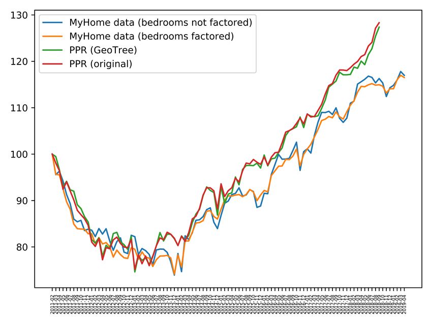
drawbacks. the MyHome data (bedrooms factored) index appearing the
smoothest time series of the four which are compared. It is
E. Enhanced Price Index
important to note that the PPR data is based upon actual sale
In order to enhance our price index model, we prepend a prices, while the MyHome data is based on listed asking prices
parameter to the geohash of each property representing the of properties which are up for sale and as such, may produce
number of bedrooms present within that property. As a result, somewhat different results.
when the GeoTree is performing the SCB computation, it will It is a well known fact that properties sell extremely well
now only match properties which are both nearby and share in spring and towards the end of the year, the former being
the same number of bedrooms. This allows the index model to the most popular period for property sales. Furthermore, the
compare the price of properties which are more similar across months towards late summer and shortly after tend to be the
the time series and thus should result in a smoother, more least busy periods in the year for selling property [28]. These
accurate measure of the change in prices over time. phenomena can be observed in Figure 2 where there is a
The technical implementation of this algorithmic enhance- dramatic increase in the listed asking prices of properties in
ment is handled almost entirely by the GeoTree automatically, the spring months and towards the end of each year, while
due to its design. As described previously, the GeoTree sees the less popular months tend to experience a slump in price
the additional parameter no differently to any other character movement. As such, the two PPR graphs and the MyHome
in the geohash and due to its placement at the start of data (bedrooms not factored) graph are following more or
the geohash, the search space will be instantly narrowed to less the same trend in price action and their graphs tend to
properties with matching number of bedrooms, x, by taking meet often, however, the majority of the price action in the
the x branch in the tree at the first step of traversal. MyHome data graphs tends to wait for the popular selling
months. The PPR graph does not experience these phenomena
VI. R ESULTS
as selling property can be a long, protracted process and due
We ran the algorithm on the MyHome data without factoring to a myriad of factors such as price bidding, paperwork, legal
any additional parameters as a control step. We then created hurdles, mortgage applications and delays in reporting, final
a GeoTree with geohash+ entries consisting of the number sale notifications can happen outside of the time period in
of bedrooms in the house prepended to the geohash for the which the sale price is agreed between buyer and seller.
property.
A. Comparison of Time Series VII. C ONCLUSION
Table I shows the performance metrics previously described
applied to the algorithms discussed in this paper: Original The introduction of bedroom factoring as an additional
PPR, PPR with GeoTree, MyHome without bedroom factoring parameter in the pairing of nearby properties has been shown
and MyHome with bedroom factoring. While both the standard to have a profound impact on the smoothness of the mix-
deviation of the differences and the MSM show that some adjusted median property price index, which was already
smoothness is sacrificed by the GeoTree implementation of the shown to outperform a popularly used implementation of
PPR algorithm, the index running on MyHome’s data without the hedonic regression model. This improvement was made
bedroom factoring approximately matches the smoothness of possible due to the acquisition of a richer data set and the
the original algorithm. Furthermore, when bedroom factoring development of the GeoTree structure, which greatly increased
is introduced, the algorithm produces by far the smoothest the performance of the algorithm. There is future potential for
index, with the standard deviation of the differences being the introduction of further property characteristics (such as
26.2% lower than the PPR (original) algorithm presented in the number of bedrooms, property type etc.) in the proximity
[5], while the MSM sits at 58.2% lower. matching part of the algorithm, should such data be acquired.
If we compare the MyHome results in isolation, we can Furthermore, the design of the data structure used en-
clearly observe that the addition of bedroom matching makes sures that minimal computational complexity is added when
a very significant impact on the index performance. While considering the technical implementation of this algorithmic
the trend of each graph is observably similar, Figure 2 adjustment. As a result of this, the index can be computed
demonstrates that month to month changes are less erratic quickly enough that it would be possible to have real-time
and appear less prone to large, spontaneous dips. Considering updates (eg. up to every 5 minutes) to the price index, if a
the smoothness metrics, the introduction of bedroom factoring sufficiently rich stream of continuous data was available to
generates a decrease of 26.8% in the standard deviation of the algorithm. Large property listing websites, such as Zillow,
the differences and a decrease of approximately 48.4% in the likely have enough live, incoming data that such an index
MSM. These results show a clear improvement by tightening would be feasible to compute at this frequency, however, this
the accuracy of property matching and are promising for the volume of data is not publicly available for testing.TABLE I: Index Comparison Statistics
Algorithm St. Dev of
St. Dev MSM
Differences
PPR (original) 16.524 2.191 23.30
PPR (GeoTree) 16.378 2.518 29.78
MyHome (without
bedrooms) 12.898 2.209 18.91
MyHome (with
bedrooms) 12.985 1.617 9.75
Fig. 2: Comparison of index on PPR and MyHome data sets, from 02-2011 to 03-2019 [data limited to 09-2018 for PPR]R EFERENCES [19] S. Jansen, P. Vries, H. Coolen, C. J. M. Lamain, and P. Boelhouwer,
“Developing a house price index for the netherlands: A practical
[1] W. E. Diewert, J. de Haan, and R. Hendriks, “Hedonic regressions application of weighted repeat sales,” The Journal of Real Estate Finance
and the decomposition of a house price index into land and structure and Economics, vol. 37, pp. 163–186, 01 2008.
components,” Econometric Reviews, vol. 34, no. 1-2, pp. 106–126, 2015. [20] G. COSTELLO and C. WATKINS, “Towards a system of local house
[Online]. Available: https://doi.org/10.1080/07474938.2014.944791 price indices,” Housing Studies, vol. 17, no. 6, pp. 857–873, 2002.
[2] K. Case, R. Shiller, and J. Quigley, “Comparing wealth effects: The [Online]. Available: https://doi.org/10.1080/02673030216001
stock market versus the housing market,” Advances in Macroeconomics, [21] R. E. Dorsey, H. Hu, W. J. Mayer, and H. chen Wang, “Hedonic versus
vol. 5, no. 1, 2001. repeat-sales housing price indexes for measuring the recent boom-bust
[3] M. Forni, M. Hallin, M. Lippi, and L. Reichlin, “Do financial cycle,” Journal of Housing Economics, vol. 19, no. 2, pp. 75 – 93,
variables help forecasting inflation and real activity in the euro area?” 2010. [Online]. Available: http://www.sciencedirect.com/science/article/
Journal of Monetary Economics, vol. 50, no. 6, pp. 1243 – 1255, pii/S105113771000015X
2003. [Online]. Available: http://www.sciencedirect.com/science/article/ [22] J. Dombrow, J. R. Knight, and C. F. Sirmans, “Aggregation bias
pii/S0304393203000795 in repeat-sales indices,” The Journal of Real Estate Finance and
Economics, vol. 14, no. 1, pp. 75–88, Jan 1997. [Online]. Available:
[4] R. Gupta and F. Hartley, “The role of asset prices in forecasting
https://doi.org/10.1023/A:1007720001268
inflation and output in south africa,” Journal of Emerging Market
[23] N. Prasad and A. Richards, “Improving median housing price
Finance, vol. 12, no. 3, pp. 239–291, 2013. [Online]. Available:
indexes through stratification,” Journal of Real Estate Research,
https://doi.org/10.1177/0972652713512913
vol. 30, no. 1, pp. 45–72, 2008. [Online]. Available: https:
[5] P. Maguire, R. Miller, P. Moser, and R. Maguire, “A robust house
//ideas.repec.org/a/jre/issued/v30n12008p45-72.html
price index using sparse and frugal data,” Journal of Property
[24] N. O’Hanlon, “Constructing a national house price index for
Research, vol. 33, no. 4, pp. 293–308, 2016. [Online]. Available:
ireland,” Journal of the Statistical and Social Inquiry Society
https://doi.org/10.1080/09599916.2016.1258718
of Ireland, vol. 40, pp. 167–196, 2011. [Online]. Available:
[6] V. Plakandaras, R. Gupta, P. Gogas, and T. Papadimitriou, “Forecasting http://hdl.handle.net/2262/62349
the u.s. real house price index,” Rimini Centre for Economic [25] MyHomeLtd. Accessed: 2019-05-31. [Online]. Available: http://www.
Analysis, Working Paper series 30-14, Nov 2014. [Online]. Available: myhome.ie
https://ideas.repec.org/p/rim/rimwps/30 14.html [26] D. P. McMillen, “Neighborhood house price indexes in Chicago:
[7] J. R. Hernando, Humanizing Finance by Hedging Property a Fourier repeat sales approach,” Journal of Economic Geography,
Values. Emerald Publishing Limited, 2018, ch. 10, pp. 183– vol. 3, no. 1, pp. 57–73, 01 2003. [Online]. Available: https:
204. [Online]. Available: https://www.emeraldinsight.com/doi/abs/10. //doi.org/10.1093/jeg/3.1.57
1108/S0196-382120170000034015 [27] J. M. Clapp, H. Kim, and A. E. Gelfand, “Predicting spatial patterns
[8] A. Jadevicius and S. Huston, “Arima modelling of lithuanian of house prices using lpr and bayesian smoothing,” Real Estate
house price index,” International Journal of Housing Markets and Economics, vol. 30, no. 4, pp. 505–532, 2002. [Online]. Available:
Analysis, vol. 8, no. 1, pp. 135–147, 2015. [Online]. Available: https://onlinelibrary.wiley.com/doi/abs/10.1111/1540-6229.00048
https://doi.org/10.1108/IJHMA-04-2014-0010 [28] L. Paci, M. A. Beamonte, A. E. Gelfand, P. Gargallo, and M. Salvador,
[9] P. Klotz, T. C. Lin, and S.-H. Hsu, “Modeling property bubble “Analysis of residential property sales using spacetime point patterns,”
dynamics in greece, ireland, portugal and spain,” Journal of European Spatial Statistics, vol. 21, pp. 149 – 165, 2017. [Online]. Available:
Real Estate Research, vol. 9, no. 1, pp. 52–75, 2016. [Online]. http://www.sciencedirect.com/science/article/pii/S2211675317300143
Available: https://doi.org/10.1108/JERER-11-2014-0038
[10] P. Englund, M. Hwang, and J. M. Quigley, “Hedging housing
risk*,” The Journal of Real Estate Finance and Economics,
vol. 24, no. 1, pp. 167–200, Jan 2002. [Online]. Available:
https://doi.org/10.1023/A:1013942607458
[11] R. Miller and P. Maguire, “GeoTree: a data structure for constant time
geospatial search enabling a real-time mix-adjusted median property
price index,” arXiv e-prints, p. arXiv:2008.02167, Aug. 2020.
[12] J. F. Kain and J. M. Quigley, “Measuring the value of housing quality,”
Journal of the American Statistical Association, vol. 65, no. 330, pp.
532–548, 1970. [Online]. Available: https://www.tandfonline.com/doi/
abs/10.1080/01621459.1970.10481102
[13] Y. M. Goh, G. Costello, and G. Schwann, “Accuracy and robustness
of house price index methods,” Housing Studies, vol. 27, no. 5, pp.
643–666, 2012. [Online]. Available: https://doi.org/10.1080/02673037.
2012.697551
[14] S. Bourassa, M. Hoesli, and J. Sun, “A simple alternative house price
index method,” Journal of Housing Economics, vol. 15, no. 1, pp. 80–97,
3 2006.
[15] B. Case, H. O. Pollakowski, and S. M. Wachter, “On choosing
among house price index methodologies,” Real Estate Economics,
vol. 19, no. 3, pp. 286–307, 1991. [Online]. Available: https:
//onlinelibrary.wiley.com/doi/abs/10.1111/1540-6229.00554
[16] M. J. Bailey, R. F. Muth, and H. O. Nourse, “A regression method for
real estate price index construction,” Journal of the American Statistical
Association, vol. 58, no. 304, pp. 933–942, 1963. [Online]. Available:
https://www.tandfonline.com/doi/abs/10.1080/01621459.1963.10480679
[17] K. E. Case and R. J. Shiller, “Prices of single family homes since
1970: New indexes for four cities,” National Bureau of Economic
Research, Working Paper 2393, September 1987. [Online]. Available:
http://www.nber.org/papers/w2393
[18] P. de Vries, J. de Haan, E. van der Wal, and G. Marin, “A house price
index based on the spar method,” Journal of Housing Economics, vol. 18,
no. 3, pp. 214 – 223, 2009, special Issue on Owner Occupied Housing
in National Accounts and Inflation Measures. [Online]. Available:
http://www.sciencedirect.com/science/article/pii/S1051137709000308You can also read