POLICY INSIGHTS FROM COMPARING CARBON PRICING MODELING SCENARIOS
←
→
Page content transcription
If your browser does not render page correctly, please read the page content below

THE CLIMATE AND ENERGY
                                     ECONOMICS PROJECT

   CLIMATE AND ENERGY ECONOMICS DISCUSSION PAPER | MAY 7, 2019

POLICY INSIGHTS FROM COMPARING CARBON PRICING
              MODELING SCENARIOS

          ALEXANDER R. BARRON    MARC A. C. HAFSTEAD       ADELE C. MORRIS

      |   Smith College          Resource for the Future   Brookings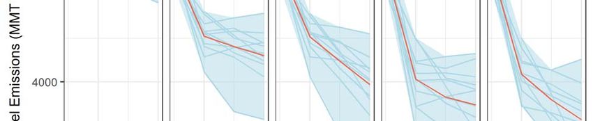

POLICY INSIGHTS FROM COMPARING CARBON
PRICING MODELING SCENARIOS
MAY 7, 2019
ALEXANDER R. BARRON
Smith College
MARC A. C. HAFSTEAD
Resource for the Future
ADELE C. MORRIS
The Brookings Institution
This discussion paper summarizes results from the Stanford Energy Modeling Forum study on U.S. carbon price
scenarios (EMF 32). More detail on any section of this discussion paper and other results of the study appear in the
February 2018 special issue of Climate Change Economics. Content is drawn heavily from Alexander R. Barron,
Allen A. Fawcett, Marc A. C. Hafstead, James R. McFarland, and Adele C. Morris 2018 Policy Insights from the EMF
32 Study on U.S. Carbon Tax Scenarios Climate Change Economics 9:1 1840003. The authors did not receive financial
support from any firm or person for this article or from any firm or person with a financial or political interest in
this article. No author is currently an officer, director, or board member of any organization with a financial or
political interest in this article.
EXECUTIVE SUMMARY

Carbon pricing is an important policy tool for reducing greenhouse gas pollution. The Stanford
Energy Modeling Forum exercise 32 convened eleven modeling teams to project emissions,
energy, and economic outcomes of an illustrative range of economy-wide carbon price policies.
The study compared a coordinated reference scenario involving no new policies with policy
scenarios that impose a price on all fossil fuel-related carbon dioxide (CO2) emissions in the
U.S. The CO2 price scenarios begin in 2020 at $25/ton or $50/ton and rise each year over
inflation at one percent or five percent. The scenarios also vary by the use of the revenue from
the carbon pricing policy; scenarios include rebates to households and deficit neutral reductions
in marginal tax rates on capital and labor income. Across all models and policy scenarios, the
study finds that carbon pricing leads to significant reductions in CO2 emissions, the majority of
which occur in the electricity sector via the reduction of coal use. Policy effects on other
energy sources vary by model, for example owing to different technology cost assumptions
(e.g., cost of natural gas vs. wind generation). Some models translate energy shifts into changes
in conventional air pollutants, reporting declines consistent with substantial air quality benefits
from the policy scenarios.

The economic costs of the policies are expected to be modest – allowing for nearly identical
economic growth– but vary across models. These costs are offset by benefits from avoided
climate damages (which are not modeled in this study) and health benefits from reductions in
conventional air pollution. The study finds that the CO2 taxes generate significant revenue; a
$25/ton price would generate roughly $1.4 trillion over the first decade and all models
reported that emissions reductions do not significantly depend on the use of the revenue.
Using revenues to reduce capital or labor taxes reduces economy-wide costs in most models
relative to household rebates, but the estimated size of the cost reductions varies significantly
across models. Across all models that estimated impacts across households, devoting at least
some revenue to household rebates improves outcomes for low income households relative to
applying all revenue to reductions in other taxes. We focus here on results through 2030,
concluding that beyond a decade model uncertainties are too large to make quantitative results
useful for near-term policy design.

                                                1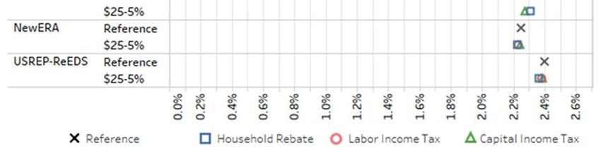
1. BACKGROUND

An extensive literature supports the economic case for imposing a price on greenhouse gas
(GHG) emissions to reduce damages from climatic disruption. In particular, a tax on the carbon
content of fossil fuels changes the relative prices of different energy sources. 1 This approach
cost effectively reduces emissions of carbon dioxide (CO2), the largest contributor to the
increase in global atmospheric concentrations of GHGs, by incentivizing shifts to lower-
emission fuels, reductions in overall energy use, and the development and deployment of lower-
cost lower-carbon technologies. The Intergovernmental Panel on Climate Change, the World
Bank, OECD, and the International Monetary Fund have all endorsed carbon pricing as a cost-
effective tool for reducing emissions (Davenport, 2016; IPCC, 2014). Some form of carbon
price is in place or under development in 46 national and 28 subnational jurisdictions (World
Bank Group, 2018).

Given the complexity of the global energy system and its links to the economy, modeling is one
of the best available tools to anticipate possible outcomes of a carbon price and explore trade-
offs between policy design choices. Since all models come with strengths and limitations, one
way to obtain a more robust understanding of the likely impacts of a policy is to analyze it with
several different models. This helps identify results that are consistent across a range of model
types (and their embedded assumptions) and those that are more sensitive to model design and
inputs. The Stanford Energy Modeling Forum (EMF) has been analyzing policy-relevant topics
with multiple models since the late 1970s. Its thirty-second study (EMF 32) convened eleven
modeling teams to analyze alternative carbon pricing policies in the United States.2

The study began with a coordinated reference scenario, which assumes no new climate policies
in the United States or other countries. To the extent feasible, modelers calibrated their
reference scenarios to the AEO 2016 Early Release No Clean Power Plan case.

Economically speaking, a carbon tax is actually two policies that operate in tandem – a price on
carbon and the use of the revenue. This study examines twelve core policy variants that vary by
price path and revenue use. Four price trajectories begin in 2020 at either $25 or $50 per ton
of CO2 and rise at either one percent or five percent over inflation per year, leveling off in
2050. All dollar values are expressed in constant 2010 dollars. The policies apply the revenue
either for direct rebates to households or to cuts in capital or labor taxes. All policy scenarios
hold the U.S. federal budget deficit constant relative to the reference scenario. Modelers did

1
  A carbon price can be implemented by a number of policy tools including a carbon tax, a cap and trade system,
or a hybrid of the two. Because the results described here could reflect the outcomes of any approach that results
in the price paths we model, we interchangeably use the terms price and tax.
2
  The scenarios in this study do not price CO2 from industrial processes (e.g. cement), terrestrial ecosystems (e.g.
forests and soils), or emissions of other GHGs (e.g. methane emissions from landfills).

                                                         2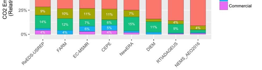
not analyze new spending or deficit reduction scenarios, which are also options available to
policymakers.

2. EMISSIONS OUTCOMES

Annual emissions

Figure 1 reports CO2 emissions projections in the reference (no new policy) scenario and four
carbon price trajectories across the eleven EMF 32 models. The red lines show the average
emissions levels across the models. The blue shaded area shows the range of model results; the
individual model trajectories appear as blue lines. For better readability, the vertical axis starts
above zero.
                      Figure 1: Annual Fossil Fuel Emissions Levels
                         (Millions of Metric Tons of CO2) by Year

Figure 1. The model with the most aggressive reductions did not report results for the $50-5%
scenario, which explains the deeper maximum reductions in the $50-1% scenario. Y-axis does
not go to zero.

                                                 3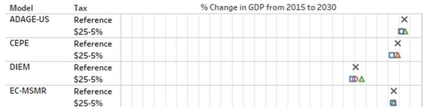
Assuming the adoption of no new climate policies in the United States or other countries, most
models projected U.S. CO2 emissions to remain flat over the coming decade, continuing their
annual contribution to rising atmospheric CO2 concentrations (the first column in Figure 1).3
The policy scenarios, labeled by their initial value in 2020 and the rate at which they escalate
each year relative to inflation, appear in the subsequent columns. They show that the larger the
carbon price, the deeper the projected emissions reductions. A CO2 price of $25 in 2020 that
rises at one percent per year reduces CO2 emissions roughly 16 to 28 percent below 2005
CO2 emissions levels4 by 2020 and 17 to 38 percent below 2005 levels by 2030. A CO2 price of
$50 in 2020 rising at 5 percent per year reduces emissions 21 to 35% below 2005 levels by
2020 and 26 to 47 percent below 2005 levels by 2030. Doubling the carbon price does not
double the reduction in emissions, reflecting an increase in the marginal costs per ton reduced
as the policy becomes more ambitious. For example, as the electricity sector becomes
decarbonized, further reductions must come from less price-responsive sectors such as
transportation and industry.

The range in emissions performance across models reflects both differences in model structure
and inherent uncertainty in key economic parameters that drive emissions reductions in these
models. Adding the full host of uncertainties around technology futures and economic growth
would increase the spread. This suggests that if policymakers want to ensure achieving a specific
national emissions target (annual or cumulative), they may need to adjust the price trajectory as
policy outcomes evolve (Aldy et al., 2017). Conversely, if policymakers want to ensure that a
particular carbon price path or range prevails, they must be flexible in the emissions outcomes.

Figure 1 shows only the scenarios in which the carbon tax revenue is returned to households in
equal rebates. Importantly, for a given carbon price path, the different uses of revenue
have little, if any, impact on emissions. This is good news, as it gives policymakers
freedom to address other policy priorities (such impacts on low-income households, the federal
deficit, infrastructure, or tax reform) without sacrificing environmental benefits. An approach
that uses the revenue to fund additional GHG reduction measures, for example in GHGs
outside the taxed sources, could produce greater overall emissions reductions than shown in
Figure 1.

All four price trajectories appear sufficient to achieve (or exceed) a 26 percent
economy-wide emissions reduction below 2005 levels by 2025 – the low end of the

3
  Model groups were asked to base their reference case projections on the Energy Information Administration’s
(EIA) Annual Energy Outlook (AEO) 2016. More current projections (AEO 2019) predict emission will slightly
decrease over time.
4
  EPA’s Greenhouse Gas Inventory currently lists 2005 fossil fuel emissions as 5777.8 MMT CO2. EIA lists energy-
related CO2 emissions (adjusted) at 5,991.6 MMT CO2.

                                                       4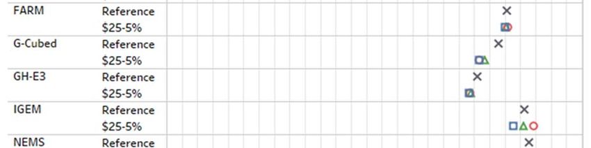
U.S. commitment in Paris.5 In scenarios not shown here, modelers found that a price
trajectory to achieve a 26 percent reduction target would begin between $9 and $22 per ton of
CO2 in 2020 and rise to between $11 and $28 by 2025.

Cumulative emissions

Because CO2’s effect in the atmosphere is long-lived and climate impacts scale with the total
CO2 concentration in the atmosphere, cumulative emissions are a better metric of
environmental benefits than emissions in any one year. By 2030 the $50 trajectories achieve
considerably greater cumulative emissions reductions, with the $50-1% scenario achieving
roughly 35 percent more total emissions reductions than the $25- 5% price path

Reductions in conventional air pollutants

As carbon prices reduce fossil fuel use, especially coal and transportation fuels, they also reduce
air pollutants like sulfur dioxide (SO2) and nitrogen oxide (NOx). Reducing these conventional
pollutants results in economically significant health benefits -- benefits that accrue within the
United States to current populations. EMF 32 models that include some of these pollutants6
report significant air quality benefits in the first decade; projected SO2 emissions from coal-fired
power decline 52 to100 percent relative to reference. The health benefits from the
average reduction in SO2 and NOx in 2025 from a $25 CO2 price are on the order of
3,500 to 8,000 avoided cases of premature mortality and 90,000 cases of
exacerbated asthma using standard epidemiological estimates (Krewski et al., 2009; Lepeule
et al., 2012) and EPA tools (Abt, 2017).

3. REVENUE AND ECONOMIC GROWTH

Revenue

In 2020, estimated gross annual revenues from the carbon tax are largely consistent across
models at about $110 billion under at $25 per ton and $200 billion at $50 per ton. In practice,
official revenue estimates would depend on factors such as the GHG sources covered by the

5
  Since not all of the models include non-CO2 emissions or land and forest carbon included in the 26% target, in
this study we assumed a target of 26% below 2005 levels for U.S. net GHG emissions can be achieved with fossil
energy CO2 emissions that are 23% below 2005 levels – this assumes a significant land sink and efficient (~26%)
reductions of non-CO2 gases. Different land use or methane emissions would require different reductions from
fossil fuel CO2.
6
  For example, these models do not allow us to quantify reductions in hazardous air pollutants.

                                                        5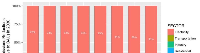
tax and Congressional Budget Office and Joint Committee on Taxation determinations about
how much the carbon tax might reduce revenues from other taxes (Elmendorf, 2009).7

With a 5 percent annual growth in the carbon tax rate, most models project revenues to rise
over time despite falling emissions. That is because the tax rate grows faster than taxable
emissions decline. On average across the models, a $25 per ton tax rising at 5% per year would
generate over $1.4 trillion in the 10-year window from 2021 to 2030.

To put the potential carbon tax revenue in perspective, in 2015 $100 billion was equal to three
percent of all federal revenue, the budget deficit was $439 billion, and the corporate income tax
raised $344 billion. The home mortgage interest deduction reduced federal revenue by an
average of $120 billion annually from 2013 to 2017, and the tax deduction for employer
payments for health insurance cost an average of $337 billion annually over the same period
(Aldy, 2017).

Economic Growth

Carbon prices affect the economy by increasing the cost of fossil fuels and through the ripple
effects across the economy. Because the cost-based effects can lower take-home benefits from
working and investing, a carbon price can increase the economic burdens of preexisting labor
and capital taxes. Using the carbon price revenue to cut other tax rates can decrease the
economic burden from those other taxes. Reducing carbon and other pollution also produces
economic benefits that could offset the economic burdens of carbon pricing, but these are not
captured in these models.

As shown in Figure 2, the projected effects of the policies on gross domestic production (GDP)
are modest. In the reference scenario, marked with an x, models project that GDP grows
between 2 and 2.5 percent annually on average between 2015 and 2030. The colored icons in
Figure 2 denote projected GDP growth rates in the carbon tax scenarios that start at $25 per
ton and rise at 5 percent annually. Different icons represent different uses of revenue; blue
squares are household rebates, red circles are labor income tax reductions, and green triangles
are capital income tax reductions. The figure shows that no matter how the revenue is
used, average GDP growth under a carbon tax is likely to be nearly identical to
average growth without the carbon tax. Indeed, the spread in GDP growth rates is
considerably larger across models than across the revenue scenarios within a model.

7
    For more on revenue, see Ramseur and Leggett (2019).

                                                       6
Figure 2: Average GDP Growth Rates

Figure 2. Average GDP growth rates over the period 2015 to 2030 in the reference case and
price scenarios with a $25/ton price rising at 5%/year for each of the models.

Some models and scenarios report higher GDP growth in the policy scenarios than in the
reference scenario, an outcome known as a double dividend. In these instances, the projected
economic benefits of the tax reduction are greater than the costs from the carbon tax.
Whether this would happen in practice is uncertain, not least because the modeling was
conducted before the 2017 legislation that significantly cut corporate tax rates.8 One could
expect the pro-growth effect of further tax cuts to be smaller than those analyzed here.

Projected GDP in 2033 is about $25 trillion in the reference scenario. In the policy scenarios in
Figure 2, the economy would reach the same level roughly three or four months later.

8
 For a more recent study that accounts for the corporate tax rate cuts see the recent work by Columbia’s Center
on Global Energy Policy (Kaufman and Gordon, 2018; Diamond and Zodrow, 2018) or Chen and Hafstead (2019).

                                                      7
4. DISTRIBUTIONAL AND ENERGY SECTOR OUTCOMES
Effects on households
Low-income households tend to spend a relatively large fraction of their income on energy, so
policymakers may be concerned that a carbon tax would be disproportionately burdensome on
them. Emerging research suggests that because low-income households receive relatively more
of their income from price-indexed social safety net programs, the impacts of carbon prices on
low-income households may not be nearly as regressive as originally thought (Cronin et al.,
2017; Goulder et al., 2018).9 Nonetheless, reducing net burden on lower-income households is
often a policy priority and it is important to understand the distributional outcomes of policy
across the income scale.
Several models in EMF 32 investigated this issue. Consistent with earlier studies, they find that
the use of revenue from a carbon price has important effects on the net impacts of the policy
across households. While tax cuts are generally more pro-growth, the benefits of the tax cuts
accrue more to higher income households, who pay more in taxes. Household rebates are the
most progressive approach; on average, rebates benefit lower income households by more than
they incur in carbon tax costs. Models reported a wide range of welfare impacts from the labor
tax cuts, suggesting significant differences in how they represent labor markets. Some modelers
showed how a blend of rebates and tax cuts can balance efficiency and equity goals (Caron et
al., 2018; Goulder et al., 2018).
Some important distributional considerations are outside this study. For example, households in
polluted areas or in places vulnerable to climatic damages are often also low-income. They may
benefit relatively more from the environmental improvements of a carbon price. Also, it makes
sense to compare the distributional outcomes of a carbon tax to those of alternative climate
policies, such as regulation. Regulatory programs can raise costs and have distributional impacts,
but they generally do not generate revenue that policymakers could use to ameliorate those
impacts.
Energy sector outcomes
One of the chief advantages of an economy-wide carbon price is that it allows emissions
reductions to come from the most cost-effective sources, regardless of sector. As shown in
Figure 3, all of the models showed emissions reductions occurring primarily (72 to 91 percent)
in the electricity sector. This is expected in the short term as changes in power generation and
plant retirements are relatively inexpensive, with lower or zero carbon generation options
9
None of the 4 models in the EMF32 study that looked at distributional impacts captured this indexing effect.
8increasingly competitive even without a carbon price. Residential housing and transportation,
on the other hand, both feature large capital stocks (i.e. houses/cars) that are slow to turn
over. Despite that, over half the models show roughly 25 percent of the reductions coming
outside the power sector. We note that models tend to lack detail on existing and future
technologies that could drive reductions in these other sectors (e.g. electrification, energy
efficiency opportunities, structural shifts) which could lead to underestimates of reductions in
those sectors (Barron, 2018).
Figure 3: Share of Emissions Reductions by Sector in 2030
Figure 3. Percentage Share of Emissions Reductions by Sector. Illustrative results for the $25-
5% scenario in 2030. Only 7 models reported detailed sectoral breakdowns.
Higher carbon prices lead to higher fossil fuel and electricity prices, in an amount that depends
on the carbon intensity of the fuels, and this leads to changes in the sources of energy. These
cost increases for consumers can be offset (completely for some income groups) with recycling
of the revenue as discussed above, and/or by adopting complementary policies to increase
deployment of energy efficiency measures and provide transportation and heating alternatives.
Figure 4 shows the energy sector outcomes for the $25-5% policy scenario (with household
rebates). The red lines show the average values across the models, the blue shaded area shows
the range of model results, and the individual model trajectories appear in blue.
9Figure 4: Energy Use by Source under the $25-5% Scenario
Coal consumption remains flat in the reference case. With the $25-5% carbon price, coal
consumption falls significantly (20 to 85 percent) by 2030. Only one model reported significant
construction of coal with carbon and capture and storage technology by 2030.
Oil use in the U.S. economy sees the smallest changes of the three major fossil fuels. The range
of oil use across models in Figure 4 is broad but with little downward trend, in part a reflection
of the limited representation of emerging alternatives to gasoline such as electric vehicles in
most models. Gasoline prices increase, on average across models, 8 percent in 2020 under a
$25/ton price and 17% under a $50/ton price – with relatively tight agreement across models.
Natural gas use remains flat in the reference case. Projections vary significantly across models
in the policy scenario, ranging from a decline of 31 percent to an increase of 24 percent above
reference levels in 2020. By 2030, some models show relatively little change in gas use while
others show significant (40 to 60 percent) reductions in gas use at a $50/ton price, presumably
by favoring renewables over gas. While natural gas usage varies significantly across models,
natural gas prices remain flat or increase as a result of the carbon price. Median natural gas
prices increase 19 percent in 2020 under a $25/ton price, while rising 34 percent under a
$50/ton price. Natural gas price projections depend heavily on assumptions about natural gas
10supply and the economics of extraction; differences in the supply of natural gas can alter these
price outcomes significantly.
Renewable Energy shows a range of responses in the models. Almost all models show
significant increases in wind energy (from a relatively low share of total energy) but very few
showed significant increases in solar – suggesting that the models in this study may not yet
reflect the current economics of solar or how it may evolve in the future (Barron, 2018).
Detailed power sector models generally show notable increases in variable renewable energy
(VRE, i.e. wind, solar), under a carbon price with shares of VRE approaching 60 percent by 2030
under the highest tax trajectory (Bistline et al., 2018). Updated renewable energy costs could
result in even higher projected shares.
Under a carbon price, electricity prices will rise wherever fossil fuels set the marginal price of
electricity. Price increases will vary significantly by region and will depend on the cost of low
carbon energy sources. In general, more coal-dependent regions such as the Southeast and
Midwest are likely to experience larger price increases, albeit from prices that are lower than in
regions like the Northeast that have already largely decarbonized electricity generation. Direct
comparison of electricity prices is currently challenging due to differences in model structure
and reporting (Bistline et al., 2018).
Trade and competitiveness
One concern about climate policy is its effects on trade and competitiveness. The EMF 32 study
applied a carbon price only in the U.S., with other regions proceeding without new climate
policies. Accordingly, the estimated trade impacts are far closer to a “worst-case” scenario than
a likely outcome (Macaluso et al., 2018). In reality, many other regions of the world, including
major U.S. trade partners Canada, Mexico, and China, have adopted or are considering carbon
prices to reduce GHG emissions. (World Bank and Ecofys 2017).
The average reduction in U.S. exports across the tax trajectories ranges from 1 percent to 2.5
percent. Energy-intensive, trade-exposed industries (EITE), which include iron and steel,
papermaking, aluminum, glass, and cement, feature a high proportion of energy consumption
and trade exposure. U.S. EITE exports fall by1.3 percent to 3.5 percent across the policy
scenarios. These shifts lead to increased emissions in other countries (leakage) which may be
reduced by border carbon adjustments or other policies (McKibbin et al., 2018).
5. UNDERSTANDING MODELS
Any policy that significantly reduces U.S. greenhouse gas emissions will require important shifts
in the energy system that powers the American economy. Anticipating this web of interactions
11within and between sectors is important to understanding the full set of potential outcomes of
a policy. Modeling involves making assumptions about how the world works, and each
assumption has its own implications. A few key limits to modeling studies like this are:
Environmental benefits are not included. A complete measure of the economic impact of a
climate policy would include both its costs and the benefits from avoiding climate damages as
well as lower (conventional) air pollution. Models used here do not produce estimates of these
air quality10 and climate benefits or capture their ripple effects through the economy,
compounding over time, the way they do other outcomes (i.e. cost).
Economies are more efficient in the models than in reality: Economic models depict a stylized
representation of the economy and do not include a vast range of inefficiencies and frictions
(financing constraints, monopolistic competition, undersupplied R&D, behavioral barriers to
energy efficiency investments, etc.). Other policies could address some of these other issues.
These models cannot currently tell us employment impacts: Most models used here assume
that “everyone who wants a job has one.” In the long run, it makes sense to assume labor
markets equilibrate. However, in the short-to-medium run, policies could dislocate some
workers in some industries, and models that assume full employment are not useful for
estimating this type of dislocation (EPA SAB, 2017).
Results are projections, not forecasts: Ideally, policymakers would like to know the exact (or
most likely) outcomes of a policy in the future, such as the price of electricity in a certain time
and place – i.e. a forecast. Models do not represent the most likely outcome, just the
outcomes given their assumptions about things like economic growth, fossil fuel prices, and
technology costs.
Models do not include much innovation: By design, models represent existing technologies that
are deployed at a scale large enough to characterize. A carbon price would spur innovation by
increasing incentives for research and development on low-carbon or energy-efficient
technologies (Hepburn et al., 2018). Indeed, that may be one of its most important outcomes.
In EMF 32, models generally fix rates of technological change to focus on the comparison of
carbon price scenarios with each other.
Focus on the first decade: While EMF 32 models produce output over several decades, we
would caution against relying on results past the next decade or so. Model parameters based on
current technologies and historical relationships between prices and economic behavior are
likely to shift significantly over longer time scales.
10
Only one model produced economy-wide air quality benefits (Woollacott, 2018)
126. CONCLUSIONS AND RECOMMENDATIONS
Modeling the impacts of a carbon price is complex given the many connections between energy
and the economy, as well as uncertainty about technology and socio-economic changes. Multi-
model studies like EMF 32 can help identify results that are robust across models. The range of
results captures one type of uncertainty; evolving technology costs, economic growth, and
other factors further increase the range of uncertainty, but we can still draw policy insights
from these results. Consistent with earlier studies (Fawcett et al., 2014), EMF 32 results
indicate that a carbon price can lead to significant reductions in CO2 emissions and that
policymakers can use both the starting tax rate and pace at which it escalates to define policy
ambition. The uncertainties here are also not a reason to delay enacting a carbon price in the
near future; any pricing policy can be modified as longer-term outcomes evolve. The literature
makes clear that delaying action increases the cost to achieve a given level of reductions
(McKibbin et al., 2014).
Consistent with earlier studies, EMF 32 shows the impacts of a carbon price will vary greatly
across energy sectors. One robust result is that the majority of the emissions reductions in the
short term will come from the electricity sector. The degree to which a carbon price can drive
reductions in other sectors, especially in the mid to long term, is harder to predict. CO2 prices
at $25/ton cause significant shifts away from coal as an energy source, and faster reductions
occur at higher prices. As modeled here, low-cost zero-carbon energy (i.e. wind) increases,
sometimes dramatically, as the carbon price increases. Changes in other non-fossil energy
sources (e.g. solar) will depend on the relative costs of competing forms of energy (e.g. wind,
natural gas).
In conclusion, our analysis of the EMF32 study offers a few broad conclusions for policymakers
interested in designing carbon pricing policies:
Analyze climate policies with the most current economic and technological
information feasible. Some outcomes are sensitive to model parameters such as economic
growth and costs of fuels, generation technologies, and batteries. Some costs are changing
rapidly; where possible, models should be up to date.
Policymakers should request multiple scenarios, ideally from multiple models. Even
with the most current information, uncertainties will remain about economic growth, fossil fuel
prices, technology costs, and other critical parameters. A robust set of sensitivity analyses from
more than one model can provide policymakers a better sense of the range of possible
outcomes for any given carbon price design.
13Models are best for insight, not foresight. There is a very natural temptation to use these
models to form expectations about costs and impacts of carbon price policies. Policymakers are
on steadier ground if they ask first what modeling can teach us about tradeoffs between policy
choices, key sensitivities, and other key design decisions and then design the policy to be robust
to variations in both assumptions and outcomes.
Request estimates of all benefits. A carbon price can produce significant benefits from both
reduced climate impacts and reduced conventional air pollution. One model in this study
directly reported economy-wide changes in some conventional air pollutants. Modelers could
develop broader capacity to estimate these benefits, and tools exist to calculate emissions
benefits using model output.
There will be surprises. The long time scale and complexity of the sectors involved only
enhances the need to think about policy designs that balance certainty for planning purposes
with the need for mechanisms (either in the executive branch or through future legislative
action) to make adjustments over time (e.g. Aldy et al., 2017).
Modeling can be improved with investment. In particular, we recommend more
investment in understanding the costs of reducing emissions outside the power sector and for
accurately projecting the costs of energy efficiency measures (Barron, 2018).
Invest in policy staff that can engage with the technical details of climate policy
analysis. Outside experts from academia, think tanks, NGOs and industry can play an
important role, but staff who understand both the technical material and the decision-makers’
priorities can best translate and interpret the information.
ACKNOWLEDGEMENTS
The authors thank the participants of the Stanford Energy Modeling Forum exercise 32 for their
work implementing these scenarios and their input in meetings and on the journal article. The
authors also thank Jameel Alsalam, Jefferson Cole, Qiuzi Chen, and Zixian Li for help with
analysis code and figures and Haleigh Anderson, Breanna Parker, and Alexandra Golikov for
helpful comments.
14REFERENCES
Abt (2017). User’s Manual for the Co-Benefits Risk Assessment (COBRA) Screening Model,
Version 3 Developed by Abt Associates for U.S. Environmental Protection Agency,
Climate Protection Partnerships Division, State and Local Climate and Energy Programs.
Aldy, JE (2017). Increasing emissions certainty under a carbon tax. Harvard Environmental Law
Review Forum, 41, 28–40.
Aldy, JE, M Hafstead, GE Metcalf, BC Murray, WA Pizer, C Reichert, and RCW III (2017).
Resolving The Inherent Uncertainty Of Carbon Taxes. Harvard Environmental Law Review
Forum, 41, 13.
Barron, AR (2018). Time to refine key climate policy models. Nature Climate Change, (8), 350–
352.
Bistline, J, E Hodson, C Rossman, J Creason, BC Murray, and AR Barron (2018). Electric sector
policy, technological change, and U.S. emissions reductions goals: Results from the EMF
32 model intercomparison Project. Energy Economics, TBD.
Caron, J, J Cole, R Goettle IV, C Onda, J McFarland, and J Woollacott (2018). Distributional
implications of a national CO 2 tax in the U.S. across income classes and regions: a
multi-model overview. Climate Change Economics, 9(1).
Chen, Y, and MAC Hafstead (2019). Using a carbon tax to meet US international climate
pledge. Climate Change Economics, 10(01), 1950002.
Cronin, JA, D Fullerton, and S Sexton (2017). Vertical and horizontal redistributions from a
carbon tax and rebate No. w23250 National Bureau of Economic Research.
Davenport, C (2016). Carbon pricing becomes a cause for the World Bank and I.M.F. The New
York Times.
Diamond, JW, and GR Zodrow (2018). The effects of carbon tax policies on the US economy
and the welfare of households Columbia SIPA GCEP.
Elmendorf, DW (2009). The budgetary treatment of emissions allowances under cap and trade
policies.
EPA SAB (2017). SAB advice on the use of economy-wide models in evaluating the social costs,
benefits, and economic impacts of air regulations No. EPA-SAB-17-012.
Fawcett, AA, LE Clarke, and JP Weyant (2014). Introduction to EMF 24. The Energy Journal,
35(01), 1–7.
Goulder, LH, MAC Hafstead, G Kim, and X Long (2018). Impacts of a Carbon Tax across US
Household Income Groups: What Are the Equity- Efficiency Trade-Offs? Working Paper
No. 18–22 Resources For the Future.
Hepburn, C, J Pless, and D Popp (2018). Encouraging Innovation that Protects Environmental
Systems: Five Policy Proposals. Review of Environmental Economics and Policy, 12(1), 154–
169.
IPCC (2014). Climate change 2014: Mitigation of climate change. Contribution of working
group III to the fifth assessment report of the Intergovernmental Panel on
Climate Change [Edenhofer, O., R. Pichs-Madruga, Y. Sokona, E. Farahani, S.
Kadner, K. Seyboth, A. Adler, I. Baum, S. Brunner, P. Eickemeier, B. Kriemann,
J. Savolainen, S. Schlömer, C. von Stechow, T. Zwickel and J.C. Minx (eds.)] Cambridge
University Press.
15Kaufman, N, and K Gordon (2018). The energy, economic, and emissions impacts of a Federal
US carbon tax Columbia SIPA GCEP.
Krewski, D, M Jerrett, RT Burnett, R Ma, E Hughes, Y Shi, MC Turner, CA Pope, G Thurston,
EE Calle, MJ Thun, B Beckerman, P DeLuca, N Finkelstein, K Ito, DK Moore, KB
Newbold, T Ramsay, Z Ross, H Shin, and B Tempalski (2009). Extended follow-up and
spatial analysis of the American Cancer Society study linking particulate air pollution and
mortality. Research Report (Health Effects Institute), (140), 5–114; discussion 115-136.
Lepeule, J, F Laden, D Dockery, and J Schwartz (2012). Chronic exposure to fine particles and
mortality: An extended follow-up of the Harvard six cities study from 1974 to 2009.
Environmental Health Perspectives, 120(7), 965–970.
Macaluso, N, S Tuladhar, J Woollacott, J McFarland, J Creason, and J Cole (2018). The impact of
carbon taxation and revenue recycling on U.S. industries. Climate Change Economics, 9(1),
1840005.
McKibbin, WJ, AC Morris, and PJ Wilcoxen (2014). The economic consequences of delay in
U.S. climate policy The Brookings Institution.
Mckibbin, WJ, AC Morris, PJ Wilcoxen, and W Liu (2018). The role of border carbon
adjustments in a u.s. carbon tax. Climate Change Economics, 09(01), 1840011.
Ramseur, JL, and JA Leggett (2019). Attaching a Price to Greenhouse Gas Emissions with a
Carbon Tax or Emissions Fee: Considerations and Potential Impacts CRS Report No.
R45625 Congressional Research Service.
Woollacott, J (2018). The economic costs and co-benefits of carbon taxation: A general
equilibrium assessment. Climate Change Economics, 9(1), TBD.
World Bank Group (2018). Carbon Pricing Dashboard. Available at
https://carbonpricingdashboard.worldbank.org/map_data. Accessed November 26, 2018.
16You can also read