Persistent topology of protein space
←
→
Page content transcription
If your browser does not render page correctly, please read the page content below
Persistent topology of protein space
                                                  W. Hamilton, J.E. Borgert, T. Hamelryck, J.S. Marron
arXiv:2102.06768v1 [q-bio.BM] 12 Feb 2021

                                                                                 Abstract
                                                    Protein fold classification is a classic problem in structural biology
                                                 and bioinformatics. We approach this problem using persistent homology.
                                                 In particular, we use alpha shape filtrations to compare a topological
                                                 representation of the data with a different representation that makes use of
                                                 knot-theoretic ideas. We use the statistical method of Angle-based Joint
                                                 and Individual Variation Explained (AJIVE) to understand similarities
                                                 and differences between these representations.

                                            1    Introduction
                                            In this study we used persistent homology (PH) and Wasserstein distances be-
                                            tween topological representations to quantify the geometry and topology of pro-
                                            tein folds. We present our analysis of the resulting geometry of “protein space”,
                                            and compare our results to existing protein structure quantification approaches,
                                            notably the Gaussian Integral Tuned (GIT) [RF03] vector representation.
                                                A major goal is to understand what insights the PH approach reveals that
                                            GIT vectors do not. We applied statistical methodology developed for multi-
                                            block data to contrast the two methods in a quantifiable and interpretable man-
                                            ner. Multi-block data refers to the setting where disparate sets of features on a
                                            common set of samples are represented by multiple data blocks. The method,
                                            Angle-based Joint and Individual Variation Explained (AJIVE) [FJHM18], de-
                                            composes the data blocks into joint and individual modes of variation. Applying
                                            AJIVE to the data blocks generated by each representation (GIT and PH) al-
                                            lows us to compare what was jointly captured by both methods and, more
                                            interestingly, contrast the individual features. In particular, clustering of the
                                            PH individual approximation finds topologically similar clusters of proteins that
                                            are not identified by the GIT representation.
                                                We computed the t-distributed stochastic neighbor embedding (t-SNE) [vdMH08]
                                            coordinates of each data matrix for visual comparison. The t-SNE method is a
                                            nonlinear dimensionality reduction technique that is useful for embedding high-
                                            dimensional data in lower dimensional space for visualization; moreover, t-SNE
                                            tends to separate data into clusters and is very popular for visualizing clustered
                                            data. Hierarchical clustering with Wards linkage on the t-SNE coordinates of
                                            the approximated PH individual matrix finds clusters of proteins in this view
                                            that are not clustered together in the GIT view, as shown by Figure 1. On

                                                                                      1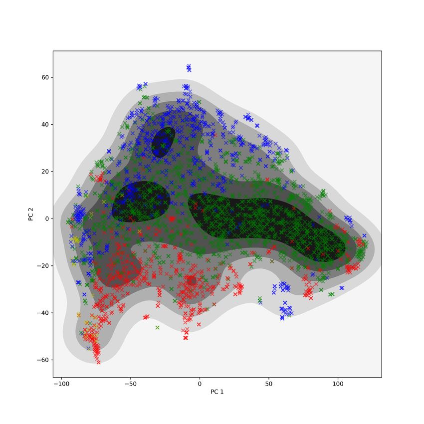
the left is the t-SNE plot of the PH individual matrix with proteins colored
by cluster label and on the right is the t-SNE plot of the original GIT vectors
matrix with the same coloring. Recall that the PH individual matrix gives us
components of the variation that are captured by PH but not by the GIT vec-
tors. Since the clusters are tight in the left plot of Figure 1 and spread out in
the right plot, we see that the topological similarities of these proteins identified
by PH are not detected by the GIT approach.

Figure 1: The 10 most homogeneous clusters from performing hierarchical clus-
tering with Wards linkage on t-SNE coordinates of PH individual matrix. On
the left, t-SNE of PH individual matrix; on the right, t-SNE coordinates of GIT
vectors. Clusters are tight in the PH individual plot but appear spread all over
in the GIT plot.

1.1    Acknowledgements
Peter Røgen provided helpful comments and suggestions regarding the GIT vec-
tor discussion. The research of Elyse Borgert and J. S. Marron were partially
supported by the grants NIH/NIAMS, P30AR072580 and NIH/NIH, R21AR074685.

2     Methods
2.1    Alpha complexes and filtrations
Alpha complexes and alpha filtrations are families of triangulated surfaces asso-
ciated to a point cloud in R2 or R3 [EKS83, Ede95], and have been proposed as
effective geometrizations of protein tertiary structure [WSS09]. In this section
we describe the construction of alpha shapes and alpha filtrations and illustrate
these objects on a protein chain in Figure 2.
    Alpha complexes are one approach to defining a combinatorial structure on
a point cloud in Euclidean space. The idea is to place a ball of some fixed radius
around each point, and connect points with an edge if the corresponding balls
intersect, connect three points with a triangle if all three balls intersect, etc.
Since we want each edge, triangle, etc., to be geometrically meaningful, we also
ask that the balls are intersected with the Voronoi cells of their centers. Recall

                                         2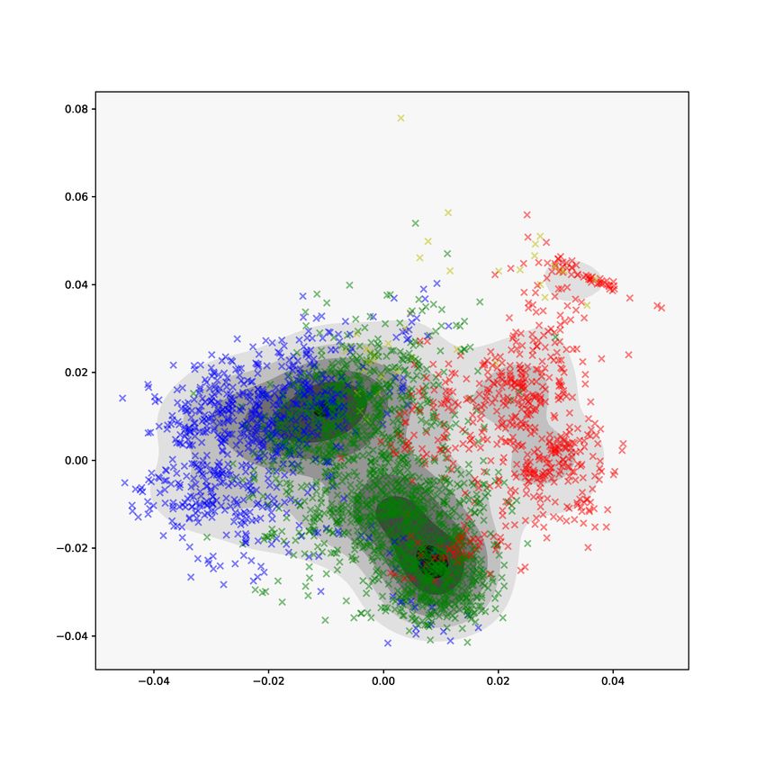
Figure 2: Left: a visualization of the protein chain 1HFE-T, referring to chain
T of the structure with identifier 1HFE in the RCSB Protein Data Bank (PDB)
[BBB+ 20]. Center-left: the point cloud of Cα atoms used to build the alpha
filtration. Center-right: the alpha shape for 1HFE-T for alpha= 1.7. The
growing balls in the alpha shape construction are indicated in red, edges between
points are indicated in black, and triangles between triples of points are shown in
blue. At this level, the 5 α-helices in 1HFE-T can be inferred from the locations
of triangles, and the hole they surround has as boundary the union of red balls.
Right: the alpha shape for 1HFE-T for alpha= 2.6. The locations of α-helices
are less clear, but the prominent hole surrounded by the α-helices is still clearly
visible.

that the Voronoi cell Vxi of a point xi in a point cloud x1 , x2 , ..., xN is the set
Vxi = {x : |xi − x| ≤ |xj − x| for j 6= i}. This intersection requirement ensures
that edges cannot “jump over” points to connect non-“adjacent” points in the
point cloud, and that no combinatorial objects of dimension higher than the
ambient space can appear. For an explicit definition of an alpha complex Xα ,
let Bα (xi ) = {x : |x − xi | ≤ α and x ∈ Vxi } be the ball of radius α centered
                                                    (k)
at xi and define the k-skeleton of Xα , denoted Xα , to be the collection of all
k-simplices in the complex:

                    Xα(k) = {(xi1 , ..., xik ) : ∩kj=1 Bα (xij ) 6= ∅}.

The alpha complex for radius α is then the union of k-skeletons for k = 1, 2, ..., d
for a point cloud in Rd .
    One natural question is: what radius of ball should we use to construct the
alpha complex? Note that if α1 < α2 , we have an inclusion of complexes Xα1 ⊂
Xα2 . This enables us to keep track of the alpha complexes for various radii and
utilizing a multiscale view of the data. Mathematically, a filtration is a family of
complexes X1 ⊂ X2 ⊂ · · · Xn ⊂ · · · such that Xi ⊂ Xi+1 , and an alpha filtration
is a family of alpha complexes parametrized by the radius of balls used in the
construction. Even though we can vary the radius continuously, new simplices in
an alpha filtration are added at discrete stages. Thus, in practice, this family of
alpha complexes for a continuously varying radius can be completely described
by a discrete family of alpha complexes Xα1 ⊂ Xα2 ⊂ · · · ⊂ Xαn for some largest
radius αn . Filtrations are computationally useful when we consider persistent
homology and intrinsic topological features across scales.
    In Figure 2 we show a 3d render of the protein chain 1HFE-T (left) [BBB+ 20],
along with the collection of Cα atoms (center-left) and two alpha complexes in

                                            3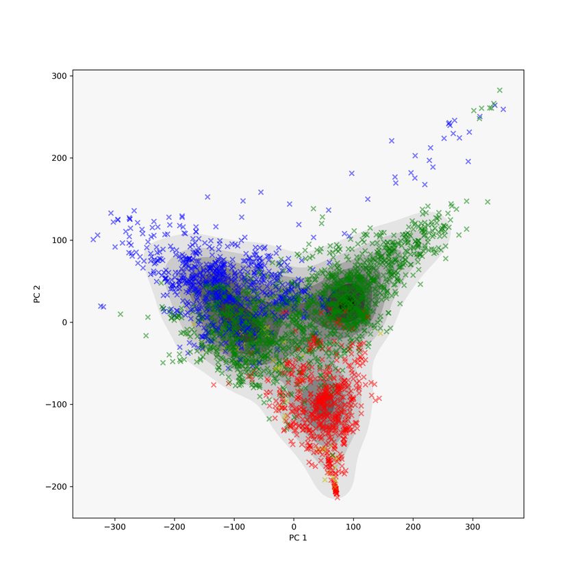
the filtration (center-right, right). Note that the average distance between adja-
cent Cα atoms along a protein is approximately 3.5 Å. Using balls of radius 1.7
(center-right), about half the average intermolecular distance, the alpha shape
has a single connected component. Moreover, the 5 α-helices of 1HFE-T are
visible as the regions with many triangles present. Using balls of radius 2.6
(right) the individual α-helices are no longer visible and the “hole” in the center
of the protein is more clearly defined.

2.2    Persistent homology
Persistent homology (PH) is a mathematical approach to quantify multiscale
topological features, such as connected components (0-dimensional), non-contractible
loops, cavities (1-dimensional), and higher-dimensional analogues. At each stage
of a filtration topological features are computed, and then matched with the cor-
responding features at other stages (if the features still exist). The collection
of all persistent features across the filtration for dimension d is referred to as
Hk , or Hk (Xα ) to emphasize the filtration used. For an introductory article see
[Ghr08, Car09], and for a textbook introduction see [EH10, Ghr14].
    The PH of a filtration is summarized as a persistence diagram (PD), some-
times called a barcode. A PD is a multiset of points {(bi , di )}i that encode
the filtration index where a feature (indexed by i) appears (bi ) and where that
feature disappears (di ). In the literature bi is called the birth time, and di the
death time. Points (bi , di ) farther from the diagonal have a larger persistence,
which is the difference between the birth and death time, and are interpreted
as intrinsic topological features. Since a PD consists of points in R2 , we can
visualize the topological features of a point cloud by plotting its PD, as shown
in the left of Figure 3; the plotted points are features, whose x-coordinates are
usually the birth time and whose y-coordinates are usually the death time. An
alternative visualization is to plot a horizontal line for each feature, whose ini-
tial x-coordinate is its birth time bi and terminal x-coordinate its death time di .
The y-axis corresponds to persistent feature index, and the user has freedom to
choose how the intervals are sorted. Popular choices are to sort the intervals
by their birth time, or by their death time. The right plot in Figure 3 shows
the barcode representation for the same PD displayed in the left plot, with the
features sorted by birth time.
    As an example of PDs and their visualization, we revisit the alpha filtration
built on 1HFE-T and consider its 1-dimensional persistent features H1 in Figure
3. In the center the alpha complex for alpha = 2.6 is displayed; note the large
“hole” visible in the center of the protein. In the left plot the PD is plotted,
and there is one feature plotted far above the diagonal colored blue. This blue
dot corresponds to the large hole in the center of 1HFE-T. In the right plot the
barcode representation is displayed. The long blue, horizontal bar corresponds
to the blue dot in the PD plot, which corresponds to the large intrinsic hole in
1HFE-T. The red, vertical bar in the barcode plot indicates the filtration value
for the alpha complex shown in the center; the red bar is a line segment with
x = 2.6.

                                        4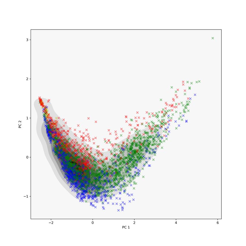
Figure 3: Left: the persistence diagram (PD) of the protein chain 1HFE-T.
Each dot corresponds to a 1-dimensional feature that appear anywhere in the
filtration, and the blue dot corresponds to the persistent “hole” seen in the
alpha shapes of 1HFE-T. Center: the alpha shape of 1HFE-T for alpha = 2.6.
Right: the barcode representation of the PD for 1HFE-T. Each horizontal line
corresponds to a 1-dimensional feature that appears anywhere in the filtrations,
and the horizontal blue line corresponds to the persistent hole in the center of
the protein. The vertical red line is x = 2.7, indicating the radius of balls used
to construct the alpha shape in the center plot. Notice that the vertical line
only intersects the horizontal red line, and none of the black lines, meaning that
the alpha shape only has one 1-dimensional feature present.
Fast algorithms exist to compute PDs using a variety of different mathe-
matical frameworks: the first algorithms used a birth-death simplex matching
method [ZC05], and recent algorithms have used discrete morse-theoretic re-
ductions to simplify the filtration [MN13] and matroid factorizations [Hen17] to
speed up or reduce the complexity of these computations. In this study we used
Dionysus [Mor] to compute PH of alpha filtrations on proteins.
2.3 Wasserstein distances
For two PDs D1 = {(bi1 , di1 )}i and D2 = {(bj2 , dj2 )}j , the q-Wasserstein distance
is defined as the cost of the optimal matching between the two point sets:
1/q
X
Wq (D1 , D2 ) := inf kx − γ(x)kq∞ ,
γ : D1∗ →D2∗
x∈D1∗
where Di∗ := Di ∪ {(x, x) : x ∈ [0, ∞)} and the infimum ranges over all bijective
maps γ : D1∗ → D2∗ [EH10, PZ20]. Points along the diagonal are included in the
matching process since PDs often contain a different number of points. Since
diagonal points have the same birth and death time, they do not correspond
to any topological features appearing in the filtration. Figure 4 illustrates an
optimal matching between two persistence diagrams: the top-left and top-right
plots contain PDs, and the bottom-left plot has the two PDs overlayed. In the
bottom-right plot, the optimal matching is shown as black lines representing
minimal length matchings of features to features, or features to the diagonal.
5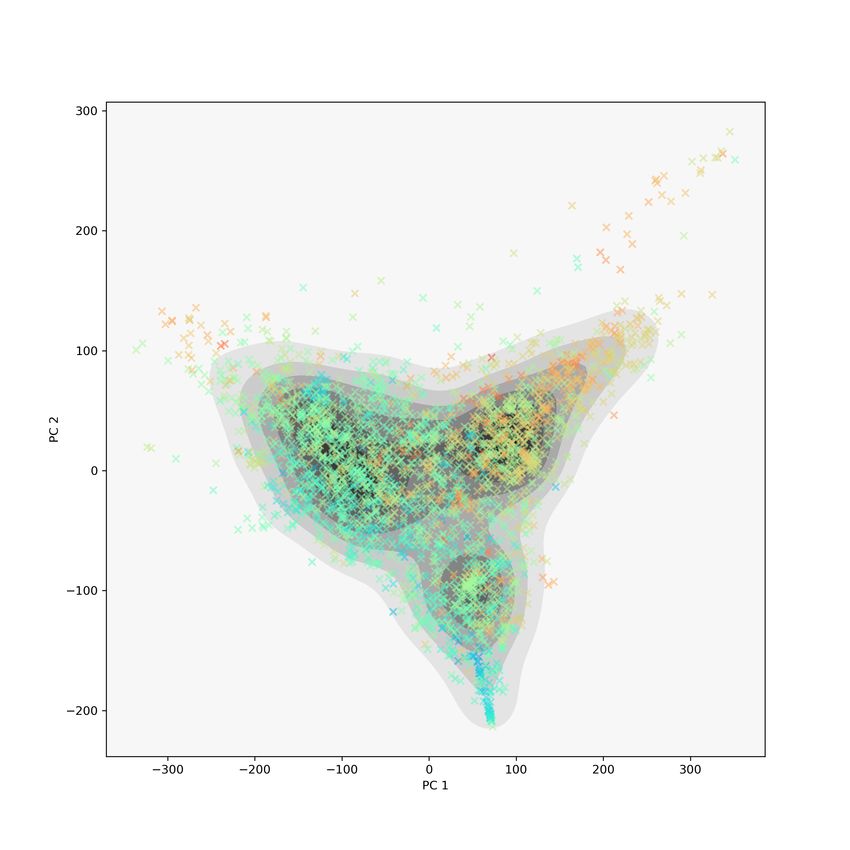
The (squared) 2-Wasserstein distance between these two PDs is the sum of the
squared L∞ norms of the black lines.

Figure 4: An illustration of the Wasserstein distance between two persistence
diagrams. Top row: two persistence diagrams. Bottom left: the persistence
diagrams overlayed. Bottom right: the optimal matching between the diagrams
indicated by solid black bars.

   Wq gives a metric on the space of PDs for 1 ≤ q ≤ ∞. In our study we
used the 2-Wasserstein distance W2 to compute distances between PDs, since
we are interested in comparing PDs based on every feature, in contrast to the
∞-Wasserstein distance which only accounts for the matched pair of PD points
that are furthest apart. We used Dionysus [Mor] for our Wasserstein distance
computations, which relies on novel geometric approaches to efficiently compute
optimal matchings [KMN17].

2.4     GIT vectors
One approach to quantifying protein structure is through representations called
Gaussian Integral Tuned (GIT) vectors. This approach interprets the structure
of a protein chain as a curve in 3D Euclidean space that is characterized using
a vector in R30 consisting of geometric invariants [RF03, Roe05] originating in
knot theory. The inspiration for this technique is through a quantity called the
writhe Wr of a closed curve γ : [0, 1] → R3 , defined as
                               Z Z
                             1
                  Wr(γ) =                         ω(t1 , t2 )dt1 dt2 ,
                            2π      0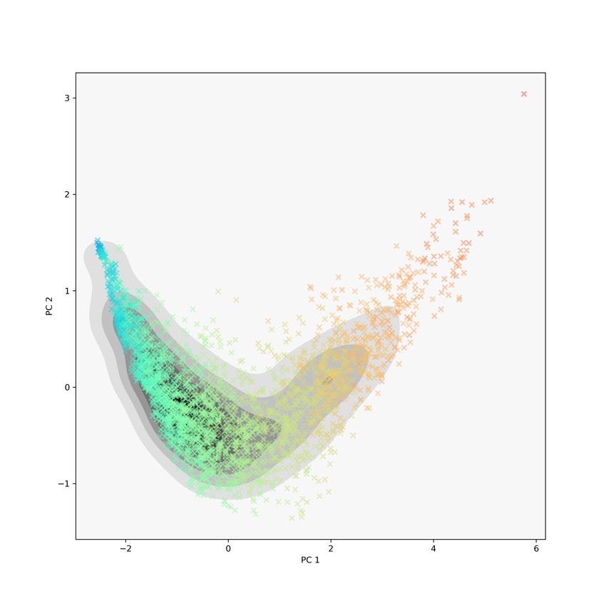
crossings ω(t1 , t2 ) seen in planar projections of the curve. For a piecewise linear
curve γ, consisting of N linear segments, the signed writhe is defined as
                                               X
                       I(1,2) (γ) = Wr(γ) =            W (i1 , i2 ),
                                                         0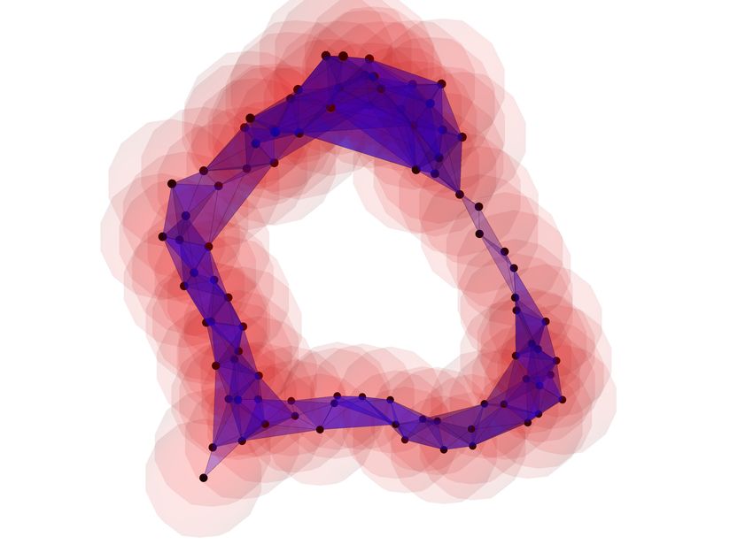
dimensionality reduction techniques throughout this study to embed the data
objects into a low-dimensional space and visualize the resulting structure.
    Two related techniques we use are Principal Component Analysis (PCA) and
Multidimensional Scaling (MDS). PCA recovers directions of maximal variation
from a collection of vectors, which are computed to minimize the vector norm
from the data to each direction [Jol02]. In practice, a singular value decomposi-
tion (SVD) is utilized to recover the directions: given a k × l data matrix X of k
data points in Rl with zero mean, the SVD of X can be written X = U ΣV , from
which we get the projections of the data onto the maximal directions S = XV T .
These scores are used to visualize Euclidean data on low-dimensional spaces that
capture the most variation. Note that PCA requires data in Euclidean space.
    MDS is a variation to PCA which is especially useful for non-Euclidean data
objects. This method seeks coordinates for each data object whose Euclidean
distances are close to given distances [Tor52]; in our case, the distances provided
are 2-Wasserstein distances between protein barcodes. When the given distances
are Euclidean, MDS and PCA return essentially the same scores. Formally,
given a collection of distances {dij } between data objects xi , xj , MDS works to
                                 P                         2
minimize the stress functional i6=j (dij − kXi − Xj k2 ) , where kXi − Xj k2 is
the vector norm between vectors Xi , Xj ; variants of this method exist which
minimize different, but related, stress functionals. Since the stress is non-linear
in the unknown coordinates, optimization techniques beyond SVD and other
linear algebraic methods need to be implemented.
    The third technique we employ is the t-distributed stochastic neighbor em-
bedding (t-SNE) [vdMH08], which finds embedding coordinates using a proba-
bilistic approach. In particular, a probability measure π1 is defined on pairs of
data objects via precomputed distances, and Euclidean coordinates X1 , ..., Xn
are computed by minimizing the Kullback-Leibler divergence between π1 and a
kernel density estimate constructed with X1 , ..., Xn as centers; in practice the
estimate is built using Gaussians. The visualisation t-SNE provides an effective
display of local aspects such as clusters and community structures, versus PCA
and MDS which are much more sensitive to global positions.

2.6    AJIVE
Angle-based Joint and Individual Variation Explained (AJIVE) [FJHM18] is a
statistical method for decomposing the joint and individual variation in a multi-
block data setting, where each data block contains a disparate set of features
taken on a common sample set. AJIVE works in three steps to implement an
angle-based solution that is efficient and guarantees identifiability. Similar to
PCA, AJIVE uses SVD to decompose data matrices and relates singular values
to principal angles to determine segmentation of joint and individual compo-
nents. First, a low-rank approximation of each data block is found by separately
applying SVD. Next, the joint components are determined by performing SVD
of the concatenated bases of the row spaces from the first step and threshold-
ing based on principal angles and bounds from perturbation theory. Finally,
joint and individual approximation matrices are given by projecting the joint

                                        8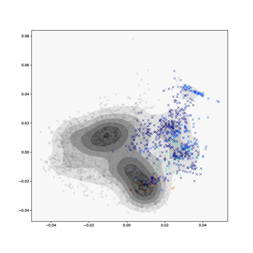
row space and its orthogonal components onto the original data blocks. AJIVE
does not require normalization and is not sensitive to potential issues arising
from heterogeneity in scale and dimension between data blocks.
    As detailed in the paper, given data matrices Xk , k ∈ {1, ..., K}, which
have the same number of samples (columns) but possibly different numbers of
features (rows), we define the following decomposition,

                        Xk = Ak + Ek = Jk + Ik + Ek .                         (1)

In this model, the Ak are deterministic low-dimensional signal matrices, Jk are
joint matrices, Ik are individual matrices, and Ek are random error matrices.
The matrices Jk representing the shared variation need not be identical but
must have a shared row space, while the matrices Ik representing individual
variation are constrained to have row spaces orthogonal to the shared row space
of the Jk .
    Segmentation of the joint spaces is based on studying the relationship be-
tween these score subspaces using theoretical bounds from Principal Angle Anal-
ysis and assessing noise effects using perturbation theory. An important point is
that by focusing on segmentation of the row spaces, the methodology captures
variation patterns across the data objects which gives interpretable meaning
of the components. Moreover, AJIVE is distinct from other methods that si-
multaneously analyze multi-block data in that it identifies individual variation
patterns. Segmentation of the individual components is a particularly important
property for the analysis done in this paper.

3     Results
3.1    Data processing
For our analysis, we used the Top8000 protein data set [CAH+ 10], consisting
of 7957 high quality protein chains from the RCSB Protein Data Bank (PDB)
[BBB+ 20]. Proteins were chosen based on the resolution of their PDB files, and
then a single chain (a linear polymer of amino acids) is selected; more details
can be found on the Top8000 repository [Lab10]. Some of the top8000 proteins
were chopped chains, meaning they were a smaller portion of a longer contiguous
chain. Other proteins in the data set had chain breaks, meaning small portions
of the polypeptides were missing due to experimental error or other reasons.
We omitted these proteins from our study.
    Since we were interested in structural features highlighted by our topological
approach, we utilized the CATH database [SDL+ 19]. CATH labels characterize
a protein’s fold using a four-fold hierarchical descriptor, consisting of Class,
Architecture, Topology and Homology. For our study we restricted our attention
to 2949 protein chains that (1) did not have any chopping (these had suffix 00 in
the top8000 directory), (2) had no chain breaks, (3) had CATH labels available,
and (4) allowed the calculation of GIT vectors. These choices were made both
for convenience and quality of data. We focused on individual chains, rather

                                        9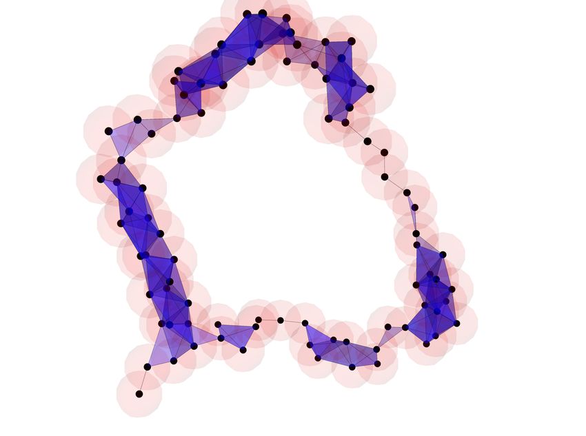
than proteins with possibly multiple chains, because fold classification is done
at the chain level. In what follows, we will refer to a protein and its chain (in the
Top8000 data set) interchangeably. Also we refer to our subset of the Top8000
data set as the CATH00 data set.
3.2 Visualization of protein space
We computed the protein H1 PDs using the persistent homology of alpha-
filtrations built on the chains’ Cα atoms. For the statistical analysis, we com-
puted all pairwise 2-Wasserstein distances between PDs and then applied MDS
and t-SNE to visualize the geometry and topology of this space of proteins.
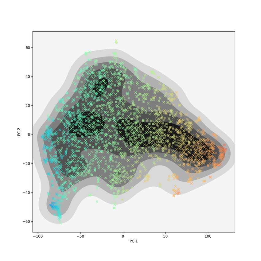
In Figure 5 we display the results of using MDS to embed the proteins into
R25 and then plot the projections onto the first two principal directions. On
the left is the kernel density estimate of the projected points, and in the middle
and on the right are the PC 1 and PC 2 scatter plots using two different colour
schemes. The colours in the middle plot are based on the sizes of each proteins’
PD (blue for fewer features in the PDs, red for more features), while the colours
in the right plot are based on Class labels: red indicates the protein consists
of α-helices, blue indicates the protein consists of β-sheets, green indicates the
protein is composed of a mix of α-helices and β-sheets, and orange indicates
the protein is without any significant content of α-helices or β-sheets. We see
separation of the proteins based on protein size along PC 1, and separation by
Class label along PC 2.
We also used t-SNE to visualize this collection of proteins, and the results
are shown in Figure 6. As in Figure 5, we show the kernel density estimate
(left) together with the 2D scatter plots of the t-SNE embedding with PD size
colours (center) and Class label colours (right). Similar to the MDS embedding,
the t-SNE embedding shows separation based on PD size and Class labels.
Figure 5: The first two PCs of the MDS coordinates using the 2-Wasserstein
metric on the full barcodes for the CATH00 data set. On the left, proteins are
coloured by barcode size; on the right, proteins are coloured by CATH-C labels.
Here we have clear separation for both barcode size and CATH-C labels
10Figure 6: For the CATH00 data set, t-SNE coordinates using the 2-Wasserstein
metric on the full barcodes, complexity 30. On the left, the kernel density
estimate for the t-SNE embedding; in the middle, proteins are coloured by
barcode size; on the right, proteins are coloured by CATH-C label. We have
clear separation for both barcode size and CATH-C labels.
3.3 Comparison of PDs to GIT vectors
For each protein we computed its GIT vector in R30 , performed PCA and pro-
jected the points onto the first two principal directions; the results are displayed
in Figure 7. On the left is the kernel density estimate for the projected coordi-
nates. In the center and on the right are scatter plots of the coordinates with
PD size and Class label colours, respectively. As in the MDS and t-SNE figures
(Figures 5 and 6), GIT vectors do a good job of sorting proteins based on their
Class labels. Unlike the previous two plots, GIT vectors do not give a strong
separation via PD size.
Figure 7: For the CATH00 data set, GIT vectors were computed and then
projected onto the first two principal directions. Left: the kernel density esti-
mate for the GIT vectors. Center: the projected GIT coordinates with PD size
colours. Right: the projected GIT coordinates with Class label colours size.
We also performed a drill-down analysis to compare how the topological
descriptors and GIT vectors grouped proteins with respect to their Class, Ar-
chitecure, and Topology labels. Figure 8 contains these results; compare to
11Figure 2 in [RF03]. The top row contains scatter plots using MDS coordinates,
while the bottom row contains scatter plots of GIT vectors. The left column
consists of the PC 1 and 2 plots of the MDS coordinates and GIT vectors, with
colors corresponding to Class labels. The center-left column contains PC 1 and
2 plots of those proteins with Class label 2 (corresponding to proteins with
mostly β-sheets), and colours correspond to Architecture labels. The red box
bounds proteins with Architecture label 60, which are proteins with a Sandwich
Architecture. In the MDS plot 38.63% of proteins in the red box do not have
Architecture label 60, while in the GIT plot 45.62% of the proteins do not have
Architecture label 60. This suggests that the Wasserstein metric clusters pro-
teins with similar CATH labels slightly more compactly than the GIT vectors
do. In the center-right column, proteins with Class and Architecture labels 2
and 60 are plotted with colors corresponding to their Topology label. The red
boxes bound proteins with Topology label 40, which are the immunoglobulin-
like proteins. In the MDS plot, 36.14% of the proteins in the red box do not
have Topology label 40, while this percentage is 47.29% in the GIT vector plot.
Again, this suggests that the global topological summaries and the Wasserstein
metric more tightly cluster proteins with similar CATH labels, as compared
to the GIT vector representation. The black colored proteins are precisely the
immunoglobulins.
Since we are most interested in aspects of the data found by PH that are not
contained in the GIT vectors, we compared the two approaches using AJIVE.
The results from each method were given as data blocks, X1 (PH) and X2
(GIT), to the AJIVE algorithm. The estimated joint components in the AJIVE
decomposition, Jˆ1 and Jˆ2 , revealed features of protein structure captured well
by both methods. More interestingly, features identified by PH that were not
identified using the GIT approach were revealed by the estimated PH individual
matrix, Iˆ1 .
The first two components of the common normalized scores (CNS) from
AJIVE are shown in Figure 9. The CNS represent a common basis of row(J), ˆ
ˆ
where row(J) denotes the estimated common score subspace of the joint matri-
ces J1 and J2 . On the left, the kernel density estimate shows two denser regions
in the center of the plot. The middle panel shows separation of the Class labels.
The green points, representing the class of mixed α-helices and β-sheets (Class
label 3), are concentrated in the dense center regions of the density estimate.
Note that the red points, which represent the α-helix class of proteins, appear
to lie in a distinct region of the density estimate and have noticeable clusters.
The right panel shows a drill-down of the red points with proteins colored by
their Architecture label, the second level of CATH classification. Separation by
Architecture label is not clear and clusters do not appear homogeneous. Exam-
ination of the CNS shows separation by Class label is a joint feature of PH and
GIT vectors, but separation by Architecture label is not well captured by the
joint components.
Next, we examined the individual block specific scores (BSS), which give the
estimated matrices Iˆ1 and Iˆ2 in the AJIVE decomposition. In particular, we are
interested in proteins that are closely related by PH but not by GIT. We com-
12Figure 8: A drilldown analysis comparing the tightness of protein clusters via
the Wasserstein metric and GIT vector representation. In the top row are
scatter plots using the MDS coordinates for the Wasserstein metric between
proteins, in the bottom row are scatter plots of GIT vectors. Left column: the
PC 1 and 2 plots of the data with Class label colors. Middle column: scatter
plots of just the Class 2 proteins (mostly β-sheets) using Architecture labels
for colors. The red boxes bound proteins with Architecture label 60 (Sandwich
Architecture). In the MDS plot (top) 38.63% of the proteins in the red box do
not have Architecture label 60, while 45.62% do not have Architecture label 60
in the GIT plot (bottom). Right column: scatter plots of just the Class 2 and
Architecture 60 proteins using Topology labels for colors. The red boxes bound
proteins with Topology label 40 (Immunoglobulin-like proteins). In the MDS
plot (top) 36.14% proteins in the red box do not have Architecture label 60,
while 47.29% do not have Architecture label 60 in the GIT plot (bottom).
puted the t-SNE coordinates of the PH individual BSS matrix and performed
hierarchical clustering on these coordinates using Wards linkage and number
of clusters n = 300. The clustering was performed on the t-SNE coordinates
rather than the original individual matrices since t-SNE gives a useful repre-
sentation for identifying and visualizing clusters. We then selected the 10 most
homogeneous clusters in terms of their Class and Architectures labels, where
homogeneity was measured by calculating the entropy in each label of each of
the 300 clusters. Figure 1 shows the results of this analysis. On the left, we see
the clusters are grouped tightly in the t-SNE coordinates of the PH individual
matrix. On the right, these same clusters in the t-SNE coordinates of the full
data block of the GIT vectors are scattered. Recall that the full data block,
X2 for the GIT vectors, is composed of both the joint and individual variation
matrices. These clusters demonstrate that PH individually finds aspects of the
data not captured by GIT vectors. Interestingly, this analysis reveals 8 proteins
completely homogeneous in their Class and Architecture label that are clustered
13Figure 9: Plots of the common normalized scores (CNS) from AJIVE. The
left plot shows the kernel density estimate of the first two components. The
middle plot shows the first two components with proteins colored by Class label.
Separation of Class label is a mode of variation common to both methods. On
the right, α-helices colored by their Architecture label.
tightly in the PH individual view but not in the GIT view.
4 Discussion
Protein fold classification can be done by considering proteins as curves in space,
characterizing these curves by their corresponding 30-dimensional GIT vectors
and subsequently identifying clusters of GIT vectors. Such clusters correspond
to proteins with similar folds. The great advantage of this method is that a com-
putationally expensive pairwise comparison of protein structures is replaced by
efficient clustering of vectors. Here we explored a similar approach, but instead
of considering protein structures as curves in Euclidean space characterized by
GIT vectors, we treat protein structures as topological objects characterized by
vectors obtained from PH.
The AJIVE analysis provides a decomposition of the data that allows us
to meaningfully compare our approach to existing methods. Moreover, the
individual components of the MDS coordinates returned by AJIVE indicate
that PH perceives aspects of protein topology different from the GIT vectors.
References
[BBB+ 20] Stephen K Burley, Charmi Bhikadiya, Chunxiao Bi, Sebastian Bit-
trich, Li Chen, Gregg V Crichlow, Cole H Christie, Kenneth Dalen-
berg, Luigi Di Costanzo, Jose M Duarte, Shuchismita Dutta, Zukang
Feng, Sai Ganesan, David S Goodsell, Sutapa Ghosh, Rachel Kramer
Green, Vladimir Guranović, Dmytro Guzenko, Brian P Hudson,
Catherine L Lawson, Yuhe Liang, Robert Lowe, Harry Namkoong,
Ezra Peisach, Irina Persikova, Chris Randle, Alexander Rose, Yana
Rose, Andrej Sali, Joan Segura, Monica Sekharan, Chenghua Shao,
14Yi-Ping Tao, Maria Voigt, John D Westbrook, Jasmine Y Young,
Christine Zardecki, and Marina Zhuravleva. RCSB Protein Data
Bank: powerful new tools for exploring 3D structures of biologi-
cal macromolecules for basic and applied research and education
in fundamental biology, biomedicine, biotechnology, bioengineering
and energy sciences. Nucleic Acids Research, 49(D1):D437–D451, 11
2020.
[CAH+ 10] Vincent B. Chen, W. Bryan Arendall, III, Jeffrey J. Headd, Daniel A.
Keedy, Robert M. Immormino, Gary J. Kapral, Laura W. Murray,
Jane S. Richardson, and David C. Richardson. MolProbity: all-
atom structure validation for macromolecular crystallography. Acta
Crystallographica Section D, 66(1):12–21, Jan 2010.
[Car09] Gunnar Carlsson. Topology and data. Bull. Amer. Math. Soc.
(N.S.), 46(2):255–308, 2009.
[Ede95] H. Edelsbrunner. The union of balls and its dual shape. Discrete
Comput. Geom., 13(3-4):415–440, 1995.
[EH10] Herbert Edelsbrunner and John L. Harer. Computational topology.
American Mathematical Society, Providence, RI, 2010. An introduc-
tion.
[EKS83] Herbert Edelsbrunner, David G. Kirkpatrick, and Raimund Seidel.
On the shape of a set of points in the plane. IEEE Trans. Inform.
Theory, 29(4):551–559, 1983.
[FJHM18] Qing Feng, Meilei Jiang, Jan Hannig, and J. S. Marron. Angle-
based joint and individual variation explained. J. Multivariate Anal.,
166:241–265, 2018.
[Ghr08] Robert Ghrist. Barcodes: the persistent topology of data. Bull.
Amer. Math. Soc. (N.S.), 45(1):61–75, 2008.
[Ghr14] R. Ghrist. Elementary Applied Topology. Createspace, 2014.
[GHR20] C. Grønbæk, T. Hamelryck, and P. Røgen. Gisa: using gauss inte-
grals to identify rare conformations in protein structures. PeerJ, 8,
2020.
[Hen17] Gregory F. Henselman. Matroids And Canonical Forms: Theory
and Applications. ProQuest LLC, Ann Arbor, MI, 2017. Thesis
(Ph.D.)–University of Pennsylvania.
[Jol02] I. T. Jolliffe. Principal component analysis. Springer Series in Statis-
tics. Springer-Verlag, New York, second edition, 2002.
[KMN17] Michael Kerber, Dmitriy Morozov, and Arnur Nigmetov. Geometry
helps to compare persistence diagrams. ACM J. Exp. Algorithmics,
22:Art. 1.4, 20, 2017.
15[Lab10] The Richardson Laboratory. The top8000 protein dataset, 2010.
[MN13] Konstantin Mischaikow and Vidit Nanda. Morse theory for filtra-
tions and efficient computation of persistent homology. Discrete
Comput. Geom., 50(2):330–353, 2013.
[Mor] D. Morozov. Dionysus.
[PZ20] Victor M Panaretos and Yoav Zemel. An invitation to statistics in
Wasserstein space. Springer Nature, 2020.
[RF03] P. Roegen and B. Fain. Automatic classification of protein structure
by using gauss integrals. PNAS, 2003.
[Roe05] P. Roegen. Evaluating protein structure descriptors and tuning gaus-
sian integral based descriptors. J. Phys.: Condens. Matter, 2005.
[SDL+ 19] I. Sillitoe, N. Dawson, T.E. Lewis, S. Das, J.G. Lees, P. Ashford,
A. Tolulope, H. M. Scholes, I. Senatorov, A. Bujan, F. C. Rodriguez-
Conde, B. Dowling, J. Thornton, and C.A. Orengo. Cath: expanding
the horizons of structure-based functional annotations for genome
sequences. Nucleic Acids Res., 2019.
[Tor52] Warren S. Torgerson. Multidimensional scaling. I. Theory and
method. Psychometrika, 17:401–419, 1952.
[vdMH08] Laurens van der Maaten and Geoffrey Hinton. Visualizing data using
t-sne. Journal of Machine Learning Research, 9(86):2579–2605, 2008.
[WSS09] P. Winter, H. Sterner, and P. Sterner. Alpha shapes and proteins.
IEEE, 2009.
[ZC05] Afra Zomorodian and Gunnar Carlsson. Computing persistent ho-
mology. Discrete Comput. Geom., 33(2):249–274, 2005.
16You can also read