Deep learning applied to NILM: is data augmentation worth for energy disaggregation? - Ecai 2020
←
→
Page content transcription
If your browser does not render page correctly, please read the page content below
9th International Conference on Prestigious Applications of Intelligent Systems – PAIS@ECAI2020
                                                        Santiago de Compostela, Spain

      Deep learning applied to NILM: is data augmentation
                worth for energy disaggregation?
                               Aurélien DELFOSSE, Georges HEBRAIL, Aimen ZERROUG 1

Abstract. Energy disaggregation (or Non-Intrusive Load Monitor-           methodology, using three different architectures for time series clas-
ing - NILM) is the task of estimating the electricity consumption of      sification or regression.
each appliance in a household from the total electricity consump-            The difficulty of NILM lies in the fact that several appliances,
tion. Disaggregated consumption gives information on each appli-          which are not always present in the house, can be used and this forces
ance and helps to find ways to reduce a household’s energy consump-       us to train several models to make multi-output prediction. Many
tion. Recent progress in deep neural networks for computer vision         NILM algorithms have been designed for high frequency data (sam-
and natural language processing gives inspiration to train general ar-    pling at kHz or even MHz) to low frequency data (1Hz- or slower)
chitectures on time series data in order to improve the state of the      like the REDD, blueED or UK Dale dataset [10] [8] sampled from 1
art on NILM, but lack of supervised data is one of the main prob-         to 6 seconds. These public datasets contain both aggregate and sub-
lems stalling the improvement of disaggregation algorithms. In this       metered energy data for each monitored house, but are not easily
paper, we introduce a new multi-agent based simulator that enables        transferable to another sampling rate or country with another energy
to generate synthetic data according to real time-use surveys. This       consumption behaviour. For example, almost all datasets will not be
synthetic dataset is used as a training set in the NILM learning pro-     reusable with the expected integration of electrical vehicles around
cess: we show that this data augmentation improves the accuracy of        the world and new behaviour with self electricity generation. In our
the disaggregation. In addition, we present four neural network archi-    experimentation, faced to the lack of 2 second data samples, which
tectures to estimate appliances consumption and establish a baseline      will be the new standard for downstream smart metering in France,
architecture on the data coming from the synthetic generator.             we introduce a Multi-Agent based Simulator (MAS), SMACH [15],
                                                                          which uses real appliances signatures to generate a synthetic dataset
                                                                          that follows the distribution of real data. This data augmentation trick
1     INTRODUCTION                                                        allows us to train networks that generalize over the real datasets and
Non-Intrusive Load Monitoring (NILM) or energy disaggregation is          unseen houses. French data is particularly complex due to the variety
the process of estimating the consumption of each individual appli-       of heating appliances, this makes disaggregation an even harder chal-
ance from the global consumption of a household. The widespread           lenge. The MAS is flexible enough to generalize over other countries
installation of smart meters in individual houses gives an opportunity    or behaviour not seen yet, and avoids data collection campaigns to
for using such a technique to help users monitor and reduce their en-     integrate significant changes in behaviour.
ergy consumption. The first application is to inform the occupant of         Since neural networks training is computationally intensive, we
the amount of energy each appliance consumes. A second applica-           use modern GPU and multi-nodes HPC environment to train several
tion is to provide a personalized feedback in case of an appliance’s      deep learning architectures adapted to time series prediction.
malfunction or inefficiency to prevent breakdowns. Finally, we can           In Section 2, we briefly review the state of the art of the NILM
warn the household’s occupant of the potential savings of differing       problem. In Section 3, we describe the data augmentation process to
appliance use to a time of the day when electricity is cheaper or has     generate synthetic data used for training. Section 4 presents the ex-
a lower carbon footprint. The last application can be associated with     perimental setup for one particular appliance, the water heater, which
solar panel system, in order to maximize the rate of self consumption     is one of the most consuming appliance. This section describes the
electricity.                                                              different generated datasets and the cross validation methodology
   The NILM problem, which was formalized in the mid-1980s                used to assess the intake of the simulator and its ability to gener-
by George Hart [5], was focused on extracting transitions between         alize, as well as the metrics. We detail the architecture choices and
steady-states. Many NILM algorithms on low frequency data (1 Hz           their performance on water heater consumption prediction using 2
of lower) followed Hart’s lead and extracted only a small number of       metrics. Section 5 presents the disaggregation results for three neural
expert features, followed by a classifier like support vector machine     network models that were trained on synthetic data and tested on real
(SVM) or K-Nearest-Neighbour(KNN). These handcrafted feature              data.
extractors are not used anymore since deep neural networks can au-
tomatically learn to extract a hierarchy of features in various objects
like raw images [17], texts [6] or time series. Deep learning for NILM    2   NILM BACKGROUND
was introduced in 2015 by Jack Kelly [9] with major progress on
                                                                          Hart’s [5] work focused on extracting transitions between steady-
state of the art models, and made a major breakthrough against old
                                                                          state considering a small number of features and used combinato-
1   ELECTRICITE DE FRANCE EDF Lab Saclay, France, email: first-           rial optimisation to find the optimal combination of appliance states
    name.lastname@edf.fr                                                  which minimises the difference between the sum of the predicted
9th International Conference on Prestigious Applications of Intelligent Systems – PAIS@ECAI2020
Santiago de Compostela, Spain
appliance power and the observed aggregate power. The second his- 3 DATA AUGMENTATION APPROACH
torical approach was proposed in 2013, and consist in using Facto-
rial HMM (FHMM) [19], [2]. The power demand of each appliance
can be modelled as the observed value of a hidden markov model. 3.1 Multi-agent based simulations of human
The hidden component of the HMMs are the states of the appliances. activity
FHMM can be viewed as an HMM where each state corresponds to
a different combination of states of each appliance. Both of these al- Gathering training data for NILM is very expensive because it re-
gorithms are bad at scaling, with a high complexity. Beyond these quires many volunteer households to monitor their energy consump-
methodologies, several improvements have been made to automati- tion with meters on several appliances. Indeed, for every household,
cally extract hierarchical sets of features. A breakthrough in super- we need both the aggregated and each sub-metered appliance to build
vised learning was made in 1989 when LeCun successfully applied the training dataset. We encounter three main difficulties in such data
neural network and back propagation to handwritten digit recogni- collection: (1) the presence of a many different appliances (oven,
tion [17]. The fully connected neural network pipeline actually learns washing machine, fridge..) which are not always available in each
automatically relevant features and makes the prediction at the same house; (2) the high variability between appliances signatures, both
time. This kind of approach took almost 20 years to become the dom- in terms of amplitude and pattern that we can meet on the appliance
inant algorithm thanks to the victory in 2012 in the ImageNet Large market ; (3) the behaviour of the household occupant, which is pretty
Scale Visual Recognition Challenge of a deep Learning approach [3] unstable according to the position and the composition of the house.
and the use of GPU (graphical processor units) which increases dras- With a constantly changing energy market, the difficulty to col-
tically computer power computation. Since 2012, deep learning in lect enough real aggregated and sub-metered data, and the necessity
most of supervised learning is considered as the state of the art ap- to study electrical vehicle consumption and develop personalized ser-
proach in many complex problems, owing to its ability to learn deep vices, the need for simulated data is on the rise. Facing this challenge,
representations of the data, and build complex parametric functions. EDF R&D developed a multi-agent simulator (MAS), which is flexi-
This flexibility has made this method a baseline approach in com- ble enough to adapt to new uses. Quentin Reynaud and Yvon Haradji
puter vision [3], natural language processing [6], time series clas- [15] proved that the integration of real time use surveys (TUS) in
sication [16] or event audio synthesis [1]. Logically, deep learning the simulator improves the realism of simulated individual behav-
becomes unavoidable to solve the NILM problem. In 2015, [9] used iors. The original TUS used in the simulator is based on 10 minutes
three neural network architectures (convolutional network, denois- activity reports (27000 reports in total) which are representative of
ing autoencoder, start&end time regressor) to predict the activation the french population’s behaviour. It helps to establish a sequence of
or consumption of several appliances. Using a mix of the UK-DALE actions for each profile in the MAS, defined by its duration, rhythm
[10] dataset sampled at 6 seconds and synthetic data, Kelly outper- and preferential period of use. In each TUS is taken in account the
formed preceding methods like combinatorial optimisation and fac- localisation, the composition of the household and the type of pric-
torial hidden Markov models [2], [5]. In his experiments, he gen- ing. These information are valuable in order to represent all the com-
erated synthetic data by randomly combining appliance signatures. plexity of the electrical consumption behaviour. This result in more
The selected appliance must fit entirely in the window presented to realistic scenarios. The output of the MAS is a sequence of activa-
the neural network and is selected with a probability of 0.5. He raised tion for each available appliances, that is adapted according to the
the point that a realistic simulator that respects temporal structure of composition and localisation of the household. Moreover, for each
appliance’s activations might increase the performance of deep neu- generated scenario, time of the year, city and household composition
ral nets compared to this naı̈ve approach which doesn’t consider this are available in order to use it as additional features in the model. The
temporal structure. simulator is flexible enough to integrate new usages like electrical ve-
Several papers were released since 2012, suggesting various ap- hicle, in addition to eleven appliances like kitchen appliances, heater,
proaches for disaggregation. [4] propose a Seq2Seq and a Seq2point vacuum cleaner, water heater or washing machine. Output scenario
method, learning the mid-point of sliding windows based on an input can be described as a table in which each column is an appliance,
short sequence, instead of the 14,400 time steps signal. This approach and rows correspond to time steps. For each time step, each column
has the advantage to manage smaller window sizes, and avoids the indicates if the appliance is activated (1) or not (0).
gradient vanishing problem [14] during the training phase. Most of The final file we consider in this study has the following format (be-
recent approaches use a LTSM layer [11],[18], which is more suit- low is the exhaustive list of each available appliances):
able for long sequence, using input, output and forget gate to manage
memory and gradient backpropagation. Finally, [13] propose to pre- 1. Time : Timestamp index (2sec).
dict the operational state change of appliances, using a smaller neural 2. vacuum cleaner : 1/0 (activate or not).
network architecture and a power threshold value to determine if the 3. water heater : 1/0.
appliance is ON/OFF. 4. washing machine : 1/0.
Since sequence modeling is still a opened challenge in machine 5. dishwasher : 1/0.
learning, an active community is trying to evaluate the best architec- 6. light : 1/0.
ture depending on the type of data [16] and has made several im- 7. fridge : 1/0.
provements since Kelly’s paper. In this paper, we evaluate some of 8. TV : 1/0.
the most promising RNN architectures adapted to long time series 9. oven : 1/0.
regression. 10. computer : 1/0.
11. electrical vehicle : 1/09th International Conference on Prestigious Applications of Intelligent Systems – PAIS@ECAI2020
Santiago de Compostela, Spain
3.2 Synthetic training data generator evaluate the interest on state of the art modeling on long time series
prediction.
We use weekly MAS simulated scenarios to build a 2 seconds re-
sampled synthetic dataset with the help of real appliances signatures
(apparent power). Appliance signatures are extracted from real data 4 EXPERIMENTAL SETUP
collected from 27 houses during our own experimentation called 4.1 Data
electric data. In comparison, the REDD dataset [8] published by
the MIT uses data coming from 6 houses. The experimentation In order to fit a baseline neural network model, we reshape the 10000
enabled us to gather aggregated and sub-metered load curves of a weekly 2 seconds generated load curves to a daily shape, which gives
large variety of appliances. An adaptation of the get activation() us a dataset of 70000 load curves with an input dimension of 43200
function created by Kelly that is available in the NILMTK [12] was time steps.
used to extract individual appliance signatures from the real dataset.
We adapted the threshold value to extract signatures specifically
for french appliances. Data generation is performed using 10000
weekly scenarios with 10 minutes time steps, and a database of
extracted signatures. These weekly scenarios are first transformed
into 2 seconds time series by repeating 0/1 appliance activation
values every 2 seconds within the 10 minutes activation/deactivation
periods. For each appliance type in a generated scenario, we select
a random appliance and then copy random signatures from this
same appliance during the scenario when the appliance is activated.
Notice that in a generated scenario, the different appliances can
come from different houses, providing use diversity in the final
dataset. This allows us to use the same scenario multiple times
and obtain a different generated output, but with a preserved
Figure 1. Example of generated aggregated and water heater curve (1 day
temporal structure also ensuring privacy. Finally, we sum all - 2 seconds sampling rate).
individual appliance consumptions to create the aggregated load
curve of the household and export the result in HDF5 format.
Each model is evaluated on a real dataset composed of 1300 daily
load curves coming from 10 houses for the water heater. The target to
Below, we present the pseudo-code for data generation based on a predict is the daily consumption of the appliance in kWh (kilo watt
MAS generated scenario s. We note: per hour). This is a regression task.
• n the time length of a scenario (t = 1..n)
• signature(i, j, k) the signature k (k = 1..ni,j ) of appliance j
(j = 1..ni ) of type i (i = 1..10)
• loadi the disaggregated load curve of appliance of type i, loadagg
the aggregated load curve
For each generated scenario s, we define the procedure to simulate
aggregated and disaggregated load curves:
1. Select scenario s
2. For each type of appliance i appearing in s
• Choose randomly an appliance j of type i
• Initialize a vector loadi of size n filled with zero values
• For each time step t which is the beginning of an activation of
type of appliance i
– Choose a random k in 1..ni,j
– Copy signature(i, j, k) to loadi from time step t to t + Figure 2. Distribution of train/test water heater consumption in kWh.
length(signature(i, j, k)) while the appliance of type i re-
mains active
P
3. Compute aggregate curve loadagg = i loadi
Note that if one wants to apply this approach to another area, it
4.2 Data preparation for cross validation
is important to use a time use survey and appliance signatures from
experiments
that country because electricity usage varies significantly between
location. As a matter of fact, different countries use different sets of In order to evaluate the performance of our regressor on the predic-
appliances and there are different usage patterns between cultures. tion of consumption based on the daily consumption curve, we gen-
Our main contribution in this publication is to highlight the need erate 10 training datasets. Each dataset excludes the signatures of
for a multi-agent simulator to generate synthetic training data and one house: the excluded house signatures are then used for creating9th International Conference on Prestigious Applications of Intelligent Systems – PAIS@ECAI2020
Santiago de Compostela, Spain
makes statitics of the data less sensitive to outliers, then we normal-
ize the result. Normalization is then just a rescaling which speeds up
training as follows:
arcsinh(α ∗ X)
X0 = (1)
α
00 X 0 − µX 0
X = (2)
σX 0
Mean and standard deviation of the training set is used to stan-
dardize the test dataset.
Figure 3. Data source for train and test generation.
4.4 Neural networks architectures
the corresponding test set. Excluding the test house’s signatures from We have tested two main architectures inspired from sequence mod-
the generated training dataset is important if we don’t want to be too elling, time series [20] [7] and signal analysis prediction. The best
optimistic and assess the ability to generalize on unseen houses. We architecture was then used to evaluate our model’s cross validation
train 10 models (one for each training dataset) and predict the house performance as explained in 4.2.
excluded from the dataset to compute the final performance. Likewise [4], we choose to model the problem with a SeqToPoint
The goal of these experiments is to determine whether a and a SeqToSeq architecture. Suppose that we are given an input
synthetic dataset can replace a real dataset and test the base- sequence (x0 , x1 , .., xT ) , and wish to predict some corresponding
line architecture capability of generalizing over curves with outputs (ŷ0i , .., ŷTi ) at each time. The Seq2Seq model consists in pre-
consumption signatures that were not used for training. dicting ŷti , that represent the estimated consumption of appliance i at
time t. The SeqToPoint architecture focuses on estimating ŷ i which
We first define the following training and test datasets: is the consumption of the whole input.
The two considered neural network architectures are the follow-
• D1 , D2 , ...D10 are the datasets of real real data corresponding to ing:
each of the 10 houses and D is the union of these datasets.
• If we choose house k = 1..10 as the house selected for testing,
• Time Distributed convolutional networks: we reshape the input
we note:
from a (43200) shape to a sequence (48, 900) of 48 timestamps.
– Dtest = Dk the test set (purple in Figure 3) This approach was successfully implemented by the University
– Dreal = D − Dk the training dataset containing real data of of Tianjin [7] to estimate machine health from a multi-sensory
all houses except house k (green in Figure 3) input. We use this architecture both for SeqToPoint and SeqToSeq
model. The prediction of the second one is calculated by summing
– Dsynth the synthetic dataset obtained with the MAS approach
all the predictions. It means that based on the model (ŷ0i , .., ŷ48
i
)=
using signatures from all houses except house k (orange in Fig- i P48 ˆi
ure 3) F (x0 , x1 , .., x48 ), we have ŷ = t=1 yt
Then we define the different training and test setups: The ConvBlock is built with 64 filters, a kernel size of 5, batch
• Baseline Learning: train a model M1 on Dsynth and test on normalization and max pooling of size 2. The activation function
Dtest . is ReLU for all layers. The Flatten layer is replaced by a Global-
• Transfer Learning FL (Full Layers): fine tune all layers of M1 AveragePooling layer. The final layer is a bi-directional LSTM of
on Dreal and test on Dtest . size 128.
• Transfer Learning 2L (2-Layers): fine tune the 2 last layers of • Temporal Convolutional Network (TCN) is directly inspired by
M1 on Dreal and test on Dtest . the Wavenet model [1] which is more convenient for long time se-
• Full Learning: train a model M2 on the union of Dsynth and ries analysis. The specificity of the TCN is to take the full signal
Dreal and test it on Dtest . as input and use causal dilated convolutions in order to respect the
• Subset learning: train a model M3 on Dreal and test on Dtest . sequence’s temporal order. [16] suggest that TCN should be con-
The training is slightly unstable due to the small size of the train- sidered as a natural starting point for sequence modeling, machine
ing dataset. translation and sentence classification, by empirically proving that
it gives a better performance than the recurrent architecture.
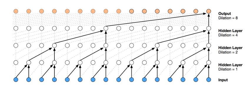
The TCN model is built with 64 filters, a kernel size of 2, a dilation
4.3 Standardization rate from 1 to 16384 (214 ) and a dropout rate of 0.2.
Individual energy consumption data is generally skewed to zero, thus
training is less stable if we use raw input data. In time series classi- Both architectures are trained with the adam optimizer with an
fication or regression, preprocessing is an important task as it influ- annealing learning rate from 0.01 to 5e10−5 . We do this by setting a
ences the way of learning. An instance preprocessing based on local more important decay rate in the optimizer in order to accelerate the
mean will focus on shape, whereas a global normalization will fa- decrease. A L2 regularizer on the weights is used with a coefficient of
vor the level of the curve. To standardize input, we first use the hy- 0.05, knowing that the network can easily over-fit faced to the small
perbolic arcsinh with a parameter α which unskews the data and dataset.9th International Conference on Prestigious Applications of Intelligent Systems – PAIS@ECAI2020
Santiago de Compostela, Spain
5 EXPERIMENTAL RESULTS
5.1 Choice of the best architecture
In order to choose the best model, the architectures presented
in Section 4.4 were tested on the whole synthetic dataset (Base-
line Learning setup defined in Section 4.2. Two variants of the
Time-Distributed architecture were also defined: (1) Time-distributed
(seq2point) (2) Time-distributed seq2seq which predicts the full se-
quence.
Table 1. Baseline regressor results.
Models MAE (kWh) SMAPE
Time-distributed 1.76 26.3%
Time-distributed seq2seq 1.82 26.8%
TCN 2.46 39.70%
Figure 4. Time-Distributed architecture.
As can be seen in Table 1, the Time-Distributed architecture ob-
tains the best score both in MAE and SMAPE. We choose this archi-
tecture to conduct the experiments described in section 3. The TCN
architecture gives promising results but was difficult to train due to
the sequence length and the small batch size. We used Horovod li-
brary to accelerate the training on GPUs.
Figures 6 and 7 show the MAE and SMAPE measures in relation
with the value of water heating consumption in each house. Note that
houses 12 and 14 consume excessively compared to other houses but
represent only 15% of the data.
Figure 5. TCN architecture.
4.5 Evaluation metrics
We use two metrics to evaluate the quality of the regression: MAE
(mean absolute error) and SMAPE (symmetric mean absolute per-
centage error) which are commonly used for regression. They have
the advantage of being robust to outliers.
n
X |yˆi − yitest | Figure 6. MAE per house for Time-Distributed network.
M AE = (3)
n
k=1
n
2 X |yˆi − yitest |
SM AP E = (4)
n |yˆi | + |yitest |
k=1
4.6 Loss function
We use a classical mean squared error loss function to train the
model, defined as follows:
n
1X
Loss = (yˆi − yi )2 (5)
n i=1
Figure 7. SMAPE per house for Time-Distributed network.
The loss function log(cosh) have been considered, knowing his
good property for managing skewness distribution of target, but
doesn’t improve results.9th International Conference on Prestigious Applications of Intelligent Systems – PAIS@ECAI2020
Santiago de Compostela, Spain
5.2 Cross-validation results REFERENCES
The Time-Distributed architecture which performed the best on the [1] Heiga Zen Karen Simonyan Oriol Vinyals Alex Graves Nal Kalch-
whole synthetic dataset was thus selected for the cross validation pro- brenner Andrew Senior Koray Kavukcuoglu. Aaron van den Oord,
Sander Dieleman, ‘Wavenet: a generative model for raw audio.’, arxiv:
cedure. We now want to highlight the fact that a model trained on our arxiv: 1609.03499, (2016).
synthetic dataset is better than one trained on our real data. [2] Michele Nati Muhammad Ali Imran. Ahmed Zoha, Alexander Gluhak,
Table 2 presents the results of the procedure for the different ‘Low-power appliance monitoring using factorial hidden markov mod-
training and test datasets, as described in Section 4.2. As for cross- els.’, IEEE, (2013).
[3] Geoffrey E. Hinton. Alex Krizhevsky, Ilya Sutskever, ‘Imagenet classi-
validation, the mean values of MAE and SMAPE were computed fication with deep convolutional neural networks.’, Nips, (2012).
over the 10 houses. [4] Zongzuo Wang Nigel Goddard Chaoyun Zhang, Mingjun Zhong and
Results show that the best performance is obtained by the Base Charles Sutton., ‘Sequence-to-point learning with neural networks for
Learning and Full Learning approaches, i.e. using the synthetic train- non-intrusive load monitoring.’, arxiv: 1612.09106, (2017).
[5] Hart G.W., ‘On intrusive appliance load monitoring.’, IEEE, (1992).
ing set. We can notice that transfer learning degrades the performance
[6] Phil Blunsom. Gábor Melis, Chris Dyer, ‘On the state of the art of eval-
of the neural network. It can be interpreted by the fact that the net- uation in neural language models.’, ICLR, (2018).
work overfits on the real houses despite the low learning rate and that [7] Peng Wang Shibin Qiao Huihui Qiao, Taiyong Wang and Lan Zhang.,
we only train the two last layers. On the other hand, as house profiles ‘A time-distributed spatio-temporal feature learning method for ma-
are highly diversified, specializing the regressor on a small set of data chine health monitoring with multi-sensor time series.’, Sensors,
(2018).
does not allow to generalize on unseen house. [8] Matthew J. Johnson J. Zico Kolter, ‘Redd: A public data set for energy
disaggregation research.’, MIT, (2011).
Table 2. Cross validation results. [9] William Knottenbelt Jack Kelly, ‘Neural nilm: Deep neural networks
applied to energy disaggregation’, arxiv: 1507.06594, (2015).
[10] William Knottenbelt Jack Kelly, ‘The uk-dale dataset, domestic
Models Data source MAE (kWh) SMAPE appliance-level electricity demand and whole-house demand from five
Base learning MAS 1.92 28.53% uk homes.’, arxiv: 1404.0284, (2015).
Transfer-learning FL real 2.55 35.83% [11] Bin Yang. Lukas Mauch, ‘A new approach for supervised power disag-
Transfer-learning 2L real 2.75 37.83% gregation by using a deep recurrent lstm network.’, IEEE, (2015).
Full learning MAS+real 1.92 29.26% [12] Oliver Parson Haimonti Dutta William Knottenbelt Alex Rogers Amar-
Subset learning real 3.13 75.71% jeet Singh Mani Srivastava Nipun Batra, Jack Kelly, ‘Nilm-tk: An open
source toolkit for non-intrusive load monitoring.’, arxiv: 1404.3878,
(2014).
[13] Samuel Cheng. Peng Xiao, ‘Neural network for nilm based on opera-
tional state change classification.’, arxiv: 1902.02675, (2019).
[14] Yoshua Bengio. Razvan Pascanu, Tomas Mikolov, ‘On the difficulty of
6 CONCLUSION training recurrent neural networks.’, arXiv : 1211.5063, (2012).
[15] Sempé F. Sabouret N. Reynaud Q., Haradji Y., ‘Using time use surveys
Multi-Agent Simulations (MAS) should be considered as a serious in multi agent based simulations of human activity.’, Proceedings of
option to solve the NILM problem and build models able to gener- the 9th International Conference on Agents and Artificial Intelligence -
Volume 1: ICAART, (2017).
alize on unseen data. This work shows that a MAS calibrated with
[16] Vladlen Koltun Shaojie Bai, J. Zico Kolter, ‘An empirical evaluation of
real time-use surveys can provide high quality synthetic data and generic convolutional and recurrent networks for sequence modeling.’,
achieve decent performance on disaggregation for high consumption arxiv: 1803.01271, (2018).
appliances. However, the quality of the generated data and regressor [17] J.S. Denker D. Henderson R.E. Howard W. Hubbard Y. Le Cun,
performance could be greatly improved if more real appliance signa- B. Boser and L.D.Jackel., ‘Backpropagation applied to handwritten zip
code recognition.’, Neural computation, (1989).
tures were available. Real annotated data is still important to assess [18] Men-Shen Tsai. Yu-Hsiu Lin, ‘A novel feature extraction method for
the quality of the prediction. Furthermore, an architecture with a mix the development of non-intrusive load monitoring system based on bp-
of convolutional and recurrent neural network are still a strong base- ann.’, arxiv: 1506.04214, (2015).
line choice for sequence modelling, even in the case of long time [19] M. I. Jordan. Z. Ghahramani, ‘Factorial hidden markov models.’, ma-
chine learning, (1997).
series prediction.
[20] Jiawei Lu Jun Xu Gang Xiao Zhipeng Shen, Yuanming Zhang, ‘Se-
riesnet:a generative time series forecasting model.’, 2018 International
Joint Conference on Neural Networks (IJCNN), (2018).You can also read


