Predictive and Descriptive Analysis for Heart Disease Diagnosis
←
→
Page content transcription
If your browser does not render page correctly, please read the page content below
Proceedings of the Federated Conference on             DOI: 10.15439/2017F219
                                   Computer Science and Information Systems pp. 155–163 ISSN 2300-5963 ACSIS, Vol. 11

           Predictive and Descriptive Analysis for Heart Disease Diagnosis
                 František Babič, Jaroslav Olejár                                      Zuzana Vantová, Ján Paralič
            Department of Cybernetics and Artificial                            Department of Cybernetics and Artificial
                           Intelligence,                                                       Intelligence,
        Faculty of Electrical Engineering and Informatics,                  Faculty of Electrical Engineering and Informatics,
            Technical university of Košice, Slovakia                            Technical university of Košice, Slovakia
           frantisek.babic@tuke.sk, jaroslav.olejar@tuke.sk                      zuzana.vantova@tuke.sk, jan.paralic@tuke.sk

     Abstract—The heart disease describes a range of conditions          The paper consists of three main sections. At first, we
  affecting our heart. It can include blood vessel diseases such as   introduce the motivation and possible approaches to support
  coronary artery disease, heart rhythm problems or and heart         the effective diagnostics of HD. The second section
  defects. This term is often used for cardiovascular disease, i.e.
  narrowed or blocked blood vessels leading to a heart attack,        describes six phases of the CRISP-DM methodology and
  chest pain or stroke. In our work, we analysed three available      related experiments. The last section concludes the paper
  data sets: Heart Disease Database, South African Heart Disease      and proposes some improvements for our future work.
  and Z-Alizadeh Sani Dataset. For this purpose, we focused on
  two directions: a predictive analysis based on Decision Trees,
  Naive Bayes, Support Vector Machine and Neural Networks;              A. Related Work
  descriptive analysis based on association and decision rules.          As HD is a very serious disease, many researchers tried to
  Our results are plausible, in some cases comparable or better
                                                                      predict it or to extract crucial risk factors. The relatively
  as in other related works
                                                                      known data sets are Cleveland, Hungarian, and Long Beach
                         I. INTRODUCTION                              VA freely available on UCI machine learning repository.
                                                                         El-Bialy et al. used all these datasets in their study [18].

  T    HE availability of various medical data leads to a
       reflection if we have some effective and powerful
  methods to process this data and extract potential new and
                                                                      At first, authors selected five common variables for each
                                                                      dataset (Cleveland, Hungarian, Long Beach VA and Statlog
                                                                      project) and applied two data mining techniques: decision
  useful knowledge. A diagnostics of different diseases               tree C4.5 and Fast Decision Tree (improved C4.5 by Jiang
  represents one of the most important challenges for data            SU and Harry Zhang). These operations resulted in accuracy
  analytics. The researchers focus their activities in several        from 69.5% (FDT, Long Beach VA data) to 78.54% (C4.5,
  directions, e.g. to generate prediction models with high            Cleveland). Next, authors merged all datasets into one
  accuracy, to extract IF-THEN rules or to investigate new            containing variables like cp, age, ca, thal, or thalach. The
  cut-off values for relevant input variables [30]. All               merging resulted in 77.5% accuracy by the C4.5 algorithm
  directions are important and can contribute to improving the        and 78.06% by FDT.
  effectiveness of the medical diagnostics.                              Verma, Srivastava, and Negi in their work [19] designed
     Heart disease (HD) is a general name for a variety of            a hybrid model for diagnosing of coronary artery disease
  diseases, conditions, and disorders that affect the heart and       (one type of HD). For this purpose, authors used data from
  the blood vessels. The symptoms depend on the specific              the Department of Cardiology at Indira Gandhi Medical
  type of this disease such coronary artery diseases, stroke,         College in Shimla in India, which contained 335 records
  heart failure, hypertensive heart disease, cardiomyopathy,          describing by 26 attributes. The authors pre-processed data
  heart arrhythmia, congenital heart disease, etc. HD is the          via correlation and features selection by particle swarm
  leading global cause of death based on a statistics of              optimization (PSO) method. For modelling authors used
  American Heart Association. The World Health                        four analytical methods: Multi-layer perceptron (MLP),
  Organization estimated that in 2012 more than 17.5 million          Multinomial logistic regression model (MLR), Fuzzy
  people died from HD (31% of all global deaths). This                unordered rule induction algorithm (FURIA) and Decision
  growing trend can be reversed by an effective prevention,           Tree C4.5. As first, they applied the MLP to the whole
  i.e. early identification of warning symptoms or typical            dataset. The obtained accuracy 77% was not satisfactory, so
  patient’s behavior leads to HD. It is a task for data analytics     they tried to improve it by MLR. This step resulted in 83.5%
  to support the diagnostic process with results in simple            accuracy. The methods FURIA and C4.5 did not offer
  understandable form for doctors or general practitioners            higher value. In the next step, authors tried to optimize data
  without deeper knowledge about algorithms and their
  applications.

IEEE Catalog Number: CFP1785N-ART c 2017, PTI                   155
156 PROCEEDINGS OF THE FEDCSIS. PRAGUE, 2017
pre-processing and tried to identify the prime risk factors specification of business goal and its transformation to the
using correlation based feature subset (CFS), selection with data mining context. The second phase focus on detailed
PSO, k-means clustering and classification or a combination data understanding through various graphical and statistical
all of these. Finally, they achieved 88.4% accuracy using methods. Data preparation is usually the most complex and
MLR and they applied proposed hybrid model on Cleveland most time-consuming phase including data aggregation,
dataset. This model improved the accuracy of classification cleaning, reduction or transformation. In modeling, different
algorithms from 8.3 % to 11.4 %. machine learning algorithms are applied to the preprocessed
Cleveland dataset is only one of several datasets typically datasets. Traditionally, this dataset is divided into training
used by researchers for analytical support of HD diagnostics. and testing sample, or analysts use 10-cross validation. The
The second is Z-Alizadeh Sani dataset collected at Tehran’s obtained results are evaluated by traditional metrics like
Shaheed Rajaei Cardiovascular, Medical and Research accuracy, ROC, precision, or recall. Next, the analysts verify
Centre. This dataset contains 303 records with 54 features. accomplish of the specified business goals. The last phase is
Alizadehsani et al. aimed to classify patients into two target devoted to the deployment of the best results in real usage
classes: suffered by coronary artery disease or normal [20]. and identification of the best or worst practices for the next
They divided the original set of variables into four groups: analytical processes.
demographic, symptoms and examination, ECG, laboratory, The decision tree is a flowchart-like tree structure, where
and echo. They focused on pre-processing phase, mainly on each non-leaf node represents a test on an attribute, each
features selection by Ginni index or Support Vector branch represents an outcome of the test, and leaf nodes
Machine. They also created several new variables like LAD represent target classes or class distributions [3]. We decided
(Left Anterior Descending), LCX (Left Circumflex) and to use this method because we were able to visualize the tree
RCA (Right Coronary Artery). For classification, authors or to extract the decision rules. The C4.5 algorithm used
used four methods: Naive Bayes, Sequential Minimal normalized information gain for splitting [4]. The C5.0
Optimization (SMO), SMO with bagging and Neural algorithm represents an improved version of the C4.5 that
network. They applied these algorithms to different pre- offers a faster generation of the model, less memory usage,
processed data sets: all original variables without three new, smaller trees with similar information value, weighting, and
all original variables with three new, only selected variables support for the boosting [5]. CTree is a non-parametric class
from the original set without three new and the selected of regression trees embedding tree-structured regression
variables from the original set with three new. The best- models into a well-defined theory of conditional inference
obtained results were 93.4% for SMO with bagging, 75.51% procedures. This algorithm does not use the traditional
for Naive Bayes, 94.08 for SMO and 88.11 for the Neural variable selection based on information gain or Ginni
network. All results were verified by 10-cross validation. coefficient but selects the variables with many possible splits
The authors extracted Typical Chest Pain, Region RWMA2, or many missing values [6]. It uses a significance test
age, Q-Wave and ST Elevation as the most important procedure. The CART (Classification and Regression Trees)
variables. algorithm builds a model by recursively partitioning the data
The same dataset was used by Yadav´s team [21] focusing space and fitting a simple prediction model within each
on an optimization of Apriori algorithm by Transaction partition [7]. The result is a binary tree using a greedy
Reduction Method (TRM). The new algorithm decreased a algorithm to select a variable and related cut-off value for
size of the candidate´s set and a number of transactional splitting with the aim to minimize a given cost function.
records in the database. The authors compared it with some Naive Bayes is a simple technique for constructing
traditional methods and obtained accuracy 93.75%; SMO classifiers that require a small number of training data to
(92.09%), SVM (89.11%), C4.5 (83.85%), Naïve Bayes estimate the parameters necessary for classification [8]. It
(80.15%). uses the probabilities of each attribute belonging to each
All mentioned works focused mainly on predictive class to make a prediction. Naive Bayes simplifies the
analysis within traditional methods like Decision Trees, calculation of probabilities by assuming that the probability
Naive Bayes, Support Vector Machine or Neural networks. of each attribute belonging to a given class value is
Next, authors tried to improve these results by suitable independent of all other attributes. To make a prediction, it
operations in pre-processing phase or by other analytical calculates the probabilities of the instance belonging to each
methods like SMO. We selected these works to set a baseline class and selects the class value with the highest probability.
for our research activities. Support Vector Machine (SVM) is a supervised machine-
learning algorithm, mostly used for classification. SVM plots
B. Methods
each record as a point in n-dimensional space (where n is a
The CRISP-DM represents the most popular methodology number of input variables). The value of each variable
for data mining and data science. This methodology defines represents a particular ordinate [9]. Then, SVM performs
six main phases from business understanding to the classification by finding a hyperplane distinguishing the two
deployment [1], [2]. The first phase deals with a target classes very well. New examples are mapped intoFRANTIŠEK BABIČ ET AL.: PREDICTIVE AND DESCRIPTIVE ANALYSIS FOR HEART DISEASE DIAGNOSIS 157
same space and predicted to a category based on which side binary classification and the second one by extraction of
of the gap they fall. association or decision rules. In data preparation phase we
Neural networks are a computational model, which is aimed to investigate possible relations between different
based on a large collection of connected simple units called combinations of variables within some statistical tests. We
artificial neurons. We will use this method if we don’t want determined a minimal 85% accuracy based on performed
to know the decision mechanism. They work like a black state of the art. For this evaluation, we used a traditional
box, i.e. we know the model is some non-linear combination confusion matrix (Table I.)
of some neurons, each of which is some non-linear TABLE I.
combination of some other neurons, but it is near impossible CONFUSION MATRIX
to say what each neuron is doing. This approach is opposite
True values
to the Decision trees or SVM. We used a feedforward neural
TP FP
network, in which the information moves in only one Predicted value
direction – forward [10]. FN TN
Association rules are a popular and well-researched
method for discovery of interesting relations between TP (true positive) – healthy people were classified
variables in (large) databases [11], [12]. The most often used correctly as healthy.
algorithm to mine association rules is Apriori [13]. FP (false positive) – healthy people were classified
Association rules analysis is a technique to uncover how incorrectly as patients with the positive diagnosis.
items are associated with each other. The Apriori principle FN (false negative) – patients with positive diagnosis were
can reduce the number of item sets we need to examine. classified incorrectly as healthy people.
We used some statistical methods to investigate possible TN (true negative) – patients with positive diagnosis were
relations between input variables themselves or between classified correctly as sick.
them and target diagnostics [14]. For this purpose, we The overall accuracy was calculated within following
applied Shapiro-Wilks normality test (null hypothesis: formula:
sample xi came from a normally distributed population [22]); TP TN
accuracy 100 (1)
2-sample Welch's t-test (the population means from the two TP FP FN TN
unrelated groups are equal [23]); Mann-Whitney-Wilcoxon
Test [29] (the two populations are equal); Pearson chi-square For evaluating the association rules, we used two
independence test (two categorical variables are independent traditional metrics: support as the proportion of health
[24]); Fisher’s Exact test (the relative proportions of one records in the dataset, which contains a combination of
variable are independent of the second variable [25]) and relevant antecedents; and confidence representing the
logistic regression [28]. Next, we used k-Nearest Neighbour proportion of health records containing antecedents and
and multiple linear regression to replace the missing values consequent two. If we define association rules as X=>Y, then
in a dataset by some plausible values [26], [27]. antecedents represent the left part of the rule (X) and the
For experiments, we used a language and environment for consequent the right part (Y).
statistical computing and graphics called R. It provides a
wide variety of statistical (linear and nonlinear modelling, B. Data Understanding and Preparation
classical statistical tests, time-series analysis, classification, We selected three available data sets devoted to the heart
clustering, etc.) and graphical techniques, and is highly diseases. The first dataset dates from 1988 and consists of
extensible1. four databases: Cleveland (303 records), Hungary (294),
Switzerland (123), and Long Beach VA (200). Each record
II. CRISP-DM is described by 14 variables (Table II.).
The distribution of target attribute in each dataset is
A. Business Understanding following: 139 patients with positive diagnostics/164 healthy
As we mentioned before, the HD diagnostics is people, 106/188, 115/8, 149/51.
complicated process containing many different input This dataset contained nearly 2 thousand missing values,
variables that need to be considered. In this case, data mainly in variable ca. For nominal attributes, we used the k-
mining can help to process and analyze available data from a NN method, for numerical multiple linear regression to solve
different point of views. The business goal is to provide an this problem. In the case of k-NN, we normalized all
application decision support for doctors and general variables to interval < -1, 1> and set up the k-value as 5.
practitioners. From data mining point of view, we can This cleaning operation changed the original distributions
transform this goal into two possible directions: predictive very slightly.
and descriptive analysis. The first one was represented by Fig. 1 visualizes a relation between resting blood pressure
and target attribute. We can say that many patients with ideal
1
https://www.r-project.org/about.html158 PROCEEDINGS OF THE FEDCSIS. PRAGUE, 2017
blood pressure (around 120) have a positive diagnosis of
heart disease.
TABLE II.
VARIABLES – DATASET 1
Name Description
age age in years (28 - 77)
sex 0- female
1- male
cp chest pain type
1-typical angina
2- atypical angina
3- non-anginal pain
4- asymptomatic
tresbps resting blood pressure (mm/Hg)
(0 - 200)
Fig. 1 Histogram (x- trestbps, y-multiplicity, green color – healthy
chol serum cholesterol (mg/dl) person, orange color – positive diagnosis)
(0 - 603)
fbs fasting blood sugar
0-false(< 120 mg/dl)
1-true (> 120 mg/dl)
restecg resting electrocardiographic results
0-normal
1- having ST-T wave abnormality
2- showing probable or definite left ventricular
hypertrophy by Estes' criteria
thalach maximum heart rate achieved (60 - 202)
exang exercise induced angina
0-no
1-yes
oldpeak ST depression induced by exercise relative to rest
(mm)
(-2.6 – 6.2)
slope the slope of the peak exercise ST segment
1-upsloping Fig. 2 Histogram (x- thalach, y-multiplicity, green color – healthy
2-flat person, orange color – positive diagnosis)
3-downsloping
ca number of major vessels colored by fluoroscopy
(0-3)
thal 3-normal
6-fixed defect
7-reversable defect
num diagnosis of heart disease (angiographic disease
status) – target attribute
0 - negative diagnosis (absence)
1 - 4 (from least serious most serious - presence)
Fig.2 visualizes a relation between maximal achieved
heart rate and target attribute. We expect that the higher
value covers people with regular exercise. Fig. 3 visualizes a
relation between sex and target attribute. The first finding
was that in the integrated dataset we had significantly more
male than female. The second was a ratio between healthy Fig. 3 Histogram (x- sex, y-multiplicity, green color – healthy person,
people and patients with positive diagnosis in both groups. orange color – positive diagnosis)FRANTIŠEK BABIČ ET AL.: PREDICTIVE AND DESCRIPTIVE ANALYSIS FOR HEART DISEASE DIAGNOSIS 159
For a better understanding of variables describing the Fig.5 visualizes a distribution of target attribute after its
EKG results, we present an example of ST segments (Fig. 4). transformation to binary one (1-4 were aggregated in 1).
The normal ST segment has a slight upward concavity. Flat,
downsloping or depressed ST segments may indicate
coronary ischemia. ST elevation may indicate transmural
myocardial infarction.
Fig. 5 Histogram (x- target attribute (absence, presence), y-
multiplicity)
Since in previous dataset we investigated the higher
occurrence of HD in male sample, as second dataset we
selected a sample of males in a heart-disease high-risk region
of the Western Cape, South Africa. It contains 462 records
Fig. 4 An example of ST segment from electrocardiography [16] described by 10 variables without missing values (Table
III.). This data sample is part of a larger dataset, described in
Next, we investigated a possibility to reduce the input set [15]. The target attribute contained 302 records of healthy
of variables. Three variables described the ECG: Restecg, persons and 160 positive diagnoses of HD.
Oldpeak, and Slope. If we visualized their distributions, the TABLE III.
first two had a low distinguish ability for target classes. We VARIABLES – DATASET 2
have omitted these two attributes from next experiments.
Name Description
Next, we investigated a relationship between nominal
age age in years (15 - 54)
variables and target attribute. For this purpose, we tried to
sbp systolic blood pressure (101 - 218)
use Pearson's Chi-squared Test and we obtained following p-
chd coronary heart disease – target attribute
values: sex (< 2.2e-16), exang (< 2.2e-16), cp (< 2.2e-16),
0 – negative diagnosis
fbs (5.972e-05), slope (< 2.2e-16), ca (8.806e-16) and thal
(< 2.2e-16). These results rejected the null hypothesis and 1 – positive diagnosis
confirmed the expected relationship. tobacco cumulative tobacco (kg)
In the case of numerical variables, we started with (0 - 31.2)
Shapiro-Wilks normality test: age (p-value = 2.268e-05), LDL low density lipoprotein cholesterol
trestbps (3.052e-15), chol (< 2.2e-16), thalach (1.906e-05). (0.98 - 15.33)
Based on this result, we choose a non-parametric Mann- adiposity measure of % body fat
Whitney-Wilcoxon Test: age (p-value = 2.2e-16), tresbps (6.74 - 42.49)
(0.001596), chol (4.941e-05), thalach (2.2e-16). If we set up obesity measure weight-to-height rations (BMI).
the 0.05 as significance level, we rejected the null hypothesis (14.70 – 46.58)
for all numeric variables, i.e. existing dependency between famhist family history of heart disease
them and target attribute. (present, absent)
Finally, we applied a logistic regression on this data. If we typea type-A behavior is characterized by an excessive
set a level for statistical significance to 0.005, the most competitive drive, impatience and anger/hostility
significant variables were sex = male (p-value = 0.000602), alcohol current alcohol consumption
slope = 2 (0.000355), ca = 1 (1.04e-05), ca = 2 (3.01e-06), (0.00 – 147.19)
ca = 3 (0.008745), cp = 4 (0.001302) and tresbps
(0.007671). Based on relevant z-values, all these variables We performed similar operations to understand the data.
increase the chance for classification into positive target Figure 5 visualizes a relation between family history of heart
class. disease (famhist) and target attribute. We can say that a160 PROCEEDINGS OF THE FEDCSIS. PRAGUE, 2017
chance to be positive diagnosed is around 50% if some heart (CAD) and normal health status. The patient is categorized
disease occurred in the family history. as CAD, if his/her diameter narrowing is greater than or
We solved an unbalanced distribution of the target equal to 50%, and otherwise as Normal. The dataset did not
attribute with an oversampling method, i.e. we re-sampled contain any missing values. In Table IV, we present only
the minority class in the training set. The result was 302 selected set of input variables as an example.
records for absent and 256 for the present. TABLE IV.
VARIABLES – DATASET 3
Name Description
age age in years (30 - 86)
0 - No
Diabetes Mellitus
1 - Yes
Fasting Blood Sugar (mg/dl) 62 - 400
Pulse Rate 50 - 100
0 - No
ST Elevation
1 - Yes
0 - No
ST Depression
1 - Yes
Low-Density Lipoprotein
18- 232
(mg/dl)
White Blood Cell 3 700 – 18 000
0 - No (BMI25)
Fig. 6 Histogram (x- famhist, y-multiplicity, green color – healthy
person, orange color – positive diagnosis) Creatine (mg/dl) 0.5 - 2.2
0 - No
Ex-Smoker
Next, we investigated potentially existing relationships 1 - Yes
between input variables and target attributes. Since we had Hemoglobin (g/dL) 8.9 - 17.6
mainly numeric variables, at first we tested if they had a 0 - No
Non-anginal CP
normal distribution. For this purpose, we used Shapiro-Wilks 1 - Yes
test with following results: age (p-value = 4.595e-13), sbp Heart disease (target 0 - Normal
(1.253e-14), tobacco (< 2.2e-16), LDL (7.148e-15), attribute) 1 - CAD
adiposity (4.245e-05), obesity (9.228e-10), typea (0.008604)
and alcohol (< 2.2e-16). In all cases, the distribution We performed similar data understanding, Fig. 7
deviated from normality based on cut-off p-value 0.05. visualizes a relation between typical chest pain and target
Based on this result, we choose a non-parametric Mann- attribute. If the patient felt chest pain, then change for heart
Whitney-Wilcoxon Test. We obtained following p-values: disease is very high. If the patient did not feel the chest pain,
age (3.364e-15), sbp (0.000214), tobacco (4.31e-12), LDL the chance for HD is still 50/50.
(6.058e-09), adiposity (1.385e-07), obesity (0.02073), typea
(0.05219) and alcohol (0.1708). If we set up the 0.05 as
significance level again, we confirmed the null hypothesis
for the two last variables, i.e. they were independent and we
omitted them.
Finally, we generated a logistic regression model based on
data with a reduced set of input variables. This model has
confirmed the importance of famhist = present (p-value =
2.68e-05), age (0.000572), tobacco (0.001847) and LDL
(0.002109). All four variables increase a chance for the
positive diagnosis of the HD.
The last dataset was Z-Alizadeh Sani Dataset containing
303 records about patients from Tehran’s Shaheed Rajaei
Cardiovascular, Medical and Research Centre [17]. Each
patient was characterized by 54 variables. These variables
were arranged in four groups: demographic, symptom and
examination, ECG, laboratory and echo features. The target
Fig. 7 Histogram (x- typical chest pain, y-multiplicity, green color –
classes were a positive diagnosis of coronary artery disease healthy person, orange color – positive diagnosis (CAD))FRANTIŠEK BABIČ ET AL.: PREDICTIVE AND DESCRIPTIVE ANALYSIS FOR HEART DISEASE DIAGNOSIS 161
disease = normal (0.00605) and Regional wall motion
We have proceeded in the same way as in the two abnormality (0.0057).
previous cases. We omitted the variables with only one This dataset was also unbalanced from the target attribute
values as e.g. Exertional CP. We started with an point of view. Therefore, we used the oversampling method
investigation of the possible normal distribution of numerical again, i.e. we re-sampled the minority class in the training
variables. We confirmed it for three variables through set. The result was 216 records for CAD and 174 for normal.
histograms (Fig. 8) and Shapiro-Wilks normality test: HB (p-
C. Modelling and Evaluation
value = 0.1301), Lymph (0.08769) and Neut (0.2627).
We applied selected data mining methods to predict the
HD and to extract relevant rules. For the prediction models,
we verified experimentally three data division to training and
testing sets (80/20, 70/30, 60/40). For each division, we
repeated the experiment for 10 times with different sampling
and in respect to the original ratio of target classes. We also
performed a stratified 10-cross validation, i.e. each fold
contained roughly the same proportions of the two types of
class labels. Finally, we applied these methods on original
datasets and with reduced sets of variables mentioned above.
Table V. presents the best-achieved results for all three
datasets.
TABLE V.
Fig. 8 Histogram (x- number of Neutrophil , y-multiplicity) THE BEST ACHIEVED PREDICTIONS
For these variables, we performed two-sample Welch's t- Name Method Accuracy (%)
test with following results: HB (p-value < 2.2e-16), Lymph Cleveland,
Decision trees 88.09
(< 2.2e-16) and Neut (< 2.2e-16). We rejected the null Hungary, Naive Bayes 86.76
hypothesis and accepted the alternative one (the population Switzerland and SVM 88.53
means are not equal), i.e. variables and target attribute were Long Beach VA
Neural networks 89.93
dependent. Decision trees 73.87
For other numerical variables, we performed the non- Naïve Bayes 71.17
South Africa Heart
parametric Mann-Whitney-Wilcoxon Test. Based on Disease SVM 73.70
significance level 0.05 we were able to reject the null
Neural networks 68.48
hypothesis for following variables: Weight (0.2137), Length
Decision trees 85.38
(0.9428), BMI (0.2537), Edema (0.3485), CR (0.3251), LDL
Z-Alizadeh Sani Naïve Bayes 83.33
(0.6088), HDL (0.5036), BUN (0.1293), Na (0.09188), WBC
Dataset SVM 86.67
(0.3672) and PLT (0.2292). It means that these variables and
target attribute were independent and we excluded them from Neural networks 86.32
our experiments.
For nominal variables, we had to use two methods: at first The first group of experiments resulted in the best model
Pearson chi-square independence test and if more than 20% generated by neural network visualized in Fig. 9. This model
of the contingency table’s cells are less than five, we used contained only reduced set of input variables. The best
Fisher’s Exact test. We omitted following variables with decision tree model was generated by CART, 10-stratified
significance level 0.05: sex (p-value = 0.2991), Current cross-validation, and all original variables. The reduced set
Smoker (0.2614), FH (0.6557), Obesity (0.8003), DLP of variables provided the same accuracy.
(0.9284), Systolic Murmur (1.0), LVH (0.5251); Ex-Smoker For the second dataset, we obtained less accurate models.
(0.7297), CRF (0.1875), CVA (1.0), Airway disease The proposed reduction of the variables did not bring any
(0.1875), Thyroid Disease (0.4138), Weak Peripheral Pulse significant improvement. Based on relevant confusion
(0.3263), Lung Rales (0.7349), Function Class (0.1405), matrices, we found out a relatively high number of records
LowTH Ang (1.0), BBB (0.307) and Poor R Progression predicted as negative, but in fact, they were positive. This is
(0.064). an important finding for future improvement.
The mentioned operations reduced an original set of input In the last case, we obtained the best model within SVM,
variables from 53 to 27. Finally, we generated a logistic which for all datasets provided one of the most accurate
regression model that confirmed the importance of variables predictions. Since it is complicated to visualize the whole
Typical Chest Pain = 1 (3.63e-05), Age (4.06e-05), Diabetes SVM model; we present an only 2-dimensional example
Mellitus (0.00321), T inversion (0.00140), Valvular heart based on attributes age and tresbps (Fig. 10).162 PROCEEDINGS OF THE FEDCSIS. PRAGUE, 2017
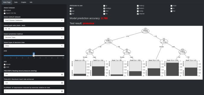
D. Deployment
The last phase is devoted to the deployment of the
evaluated and verified models into practice. We focused on
simple understandable and interpretable application to
support the diagnostic process of the heart diseases. We used
an open source R package Shiny that provides an elegant and
powerful web framework for building web applications using
R . Fig. 11 visualizes our prototype offering all analytical
features described in this paper, e.g. data understanding,
statistical tests, classification models generation and
diagnosis of a new patient.
Fig. 9 The structure of the created neural network with the best
prediction ability (input layer = 20 neurons, hidden layer = 5 neurons,
red numbers - bias)
Fig. 11 An example of supporting application
III. CONCLUSION
This paper presents the application of various statistical
and data mining methods to understand three different
medical data sets, to generate some prediction models or to
extract rules suitable for decision support during the
diagnostic process. We used some statistical tests to find out
possible existing relationships between input variables and
target attribute. Based on relevant results, we prepared the
datasets for modeling phase, in which we applied some
Fig. 10 The example of SVM prediction model (x – tresbps,y – age, selected methods as decision trees, Naive Bayes, Support
purple – positive diagnosis, cyan – negative diagnosis) Vector Machine or Apriori algorithm. In comparison with
existing studies, our results are plausible, in some cases
Finally, we discretized all numerical attributes in comparable or better. In our future work, we will focus on
accordance with the typical categories defined by existing several directions: transformation and creation of the new
medical literature. Next, we applied the Apriori algorithm to derived variables to improve the data information value;
generate association rules. These rules were very similar to investigation of the new cut-off values for selected variables,
those we extracted from the decision trees models: boosting for prediction models and e.g. cost matrix for
IF thal = reversable defect/ fixed defect AND ca = 1/2/3 unbalanced distribution
THEN HD = positive diagnosis (dataset1 – decision rules)
IF sex = male AND exang = yes AND oldpeak > 0.8 ACKNOWLEDGMENT
THEN HD = positive (dataset1 – association rules)
The work presented in this paper was partially supported
IF age < 50.05 AND tobacco > 0.46 AND typea > 68.5
by the Slovak Grant Agency of the Ministry of Education
THEN HD = positive (dataset2)
and Academy of Science of the Slovak Republic under grant
IF famhist = 1 and LDL = high THEN HD = positive
no. 1/0493/16, by the Cultural and Educational Grant
(dataset2)
Agency of the Ministry of Education and Academy of
IF Typical Chest Pain = 0 AND Age < 61 and Region
Science of the Slovak Republic under grants no. 025TUKE-
RWMA = 0/1 THEN HD = positive (dataset3)
4/2015 and no. 05TUKE-4/2017.
IF Typical Chest Pain = 1 AND VHD = mild THEN HD =
The authors would like to thank the principal investigators
positive (dataset3)
responsible for data collection: Andras Janosi, M.D.
We can conclude that the content of the generated
(Hungarian Institute of Cardiology, Budapest); William
prediction models is in accordance with the results of the
Steinbrunn, M.D. (University Hospital, Zurich); Matthias
relevant statistical tests about attributes dependency.FRANTIŠEK BABIČ ET AL.: PREDICTIVE AND DESCRIPTIVE ANALYSIS FOR HEART DISEASE DIAGNOSIS 163
Pfisterer, M.D. (University Hospital, Basel); Robert [15] J.E. Rossouw, J. du Plessis, A. Benade, P. Jordaan, J. Kotze, and
P. Jooste, “Coronary risk factor screening in three rural communities”,
Detrano, M.D., Ph.D. (V.A. Medical Center, Long Beach South African Medical Journal, vol. 64, 1983, pp. 430–436.
and Cleveland Clinic Foundation; J. Rousseauw et al. and Z- [16] R. Kreuger, “ST Segment”, ECGpedia.
Alizadeh Sani et. al. [17] R. Alizadehsani, M. J. Hosseini, Z. A. Sani, A. Gandeharioun, and
R. Boghrati, “Diagnosis of Coronary Artery Disease Using Cost-
Sensitive Algorithms”, IEEE 12th International Conference on Data
REFERENCES Mining Workshop, 2012, pp. 9–16, doi: 10.1109/ICDMW.2012.29.
[1] P. Chapman, J. Clinton, R. Kerber, T. Khabaza, T. Reinartz, [18] R. El-Bialy, M. A. Salamay, O. H. Karam, and M. E. Khalifa, "Feature
C. Shearer, and R. Wirth: “CRISP-DM 1.0 Step-by-Step Data Mining Analysis of Coronary Artery Heart Disease Data Sets", Procedia
Guide”, 2000. Computer Science, ICCMIT 2015, vol. 65, pp. 459–468, doi:
[2] C. Shearer, “The CRISP-DM Model: The New Blueprint for Data 10.1016/j.procs.2015.09.132.
Mining”, Journal of Data Ware-housing, vol. 5, no. 4, 2000, pp. 13– [19] L. Verma, S. Srivastaa, and P.C. Negi, "A Hybrid Data Mining Model
22. to Predict Coronary Artery Disease Cases Using Non-Invasive
[3] K.S. Murthy, “Automatic construction of decision tress from data: A Clinical Data", Journal of Medical Systems, vol. 40, no. 178, 2016,
multidisciplinary survey”, Data Mining and Knowledge Discovery, doi: 10.1007/s10916-016-0536-z.
1997, pp. 345–389, doi: 10.1007/s10618-016-0460-3. [20] R. Alizadehsani, J. Habibi, M. J. Hosseini, H. Mashayekhi,
[4] J. R. Quinlan, “C4.5: Programs for Machine Learning”, Morgan R. Boghrati, A. Ghandeharioun, B. Bahadorian, and Z. A. Sani, "A
Kaufmann Publishers, 1993, doi: 10.1007/BF00993309. data mining approach for diagnosis of coronary artery disease",
[5] N. Patil, R. Lathi, and V. Chitre, “Comparison of C5.0 & CART Computer Methods and Programs in Biomedicine, vol. 111, no. 1,
Classification algorithms using pruning technique”, International 2013, pp. 52-61, doi: 10.1016/j.cmpb.2013.03.004.
Journal of Engineering Research & Technology, vol. 1, no. 4, 2012, [21] Ch. Yadav, S. Lade, and M. Suman, "Predictive Analysis for the
pp. 1–5. Diagnosis of Coronary Artery Disease using Association Rule
[6] T. Hothorn, K. Hornik, and A. Zeileis, “Unbiased recursive Mining", International Journal of Computer Applications, vol. 87, no.
partitioning: A conditional inference framework”, Journal of 4, 2014, pp. 9-13.
Computational and Graphical Statistics, vol. 15, no. 3, 2006, pp. 651– [22] S. S. Shapiro, M. B. Wilk, "An analysis of variance test for normality
674, doi: 10.1198/106186006X133933. (complete samples)", Biometrika, vol. 52, no. 3–4, 1965, pp. 591–611,
[7] L. Breiman, J.H. Friedman, R.A. Olshen, Ch.J. Stone, “Classification doi: 10.1093/biomet/52.3-4.591.
and Regression Trees”, 1999, CRC Press, doi: [23] B. L. Welch, "On the Comparison of Several Mean Values: An
10.1002/cyto.990080516. Alternative Approach", Biometrika, vol. 38, 1951, pp. 330–336, doi:
[8] D. J Hand, K. Yu, “Idiot's Bayes-not so stupid after all?”, International 10.2307/2332579.
Statistical Review, vol. 69, no. 3, 2001, pp. 385–399. [24] K. Pearson, Karl, "On the criterion that a given system of deviations
doi:10.2307/1403452 from the probable in the case of a correlated system of variables is
[9] C. Cortes, V. Vapnik, "Support-vector networks", Machine Learning, such that it can be reasonably supposed to have arisen from random
vol. 20, no. 3, 1995, pp. 273–297, doi:10.1007/BF00994018. sampling", Philosophical Magazine Series 5, vol. 50, no. 302, 1900,
[10] K. Hornik, “Approximation capabilities of multilayer feedforward pp. 157–175, doi: 10.1080/14786440009463897.
networks,” Neural Networks, vol. 4, 1991, pp. 251–257, doi: [25] R. A. Fisher, "On the interpretation of χ2 from contingency tables, and
10.1016/0893-6080(91)90009-T. the calculation of P", Journal of the Royal Statistical Society, vol. 85,
[11] R. Agrawal, R. Srikant, “Fast Algorithms for Mining Association no. 1,1922, pp. 87–94, doi: 10.2307/2340521.
Rules in Large Data-bases”, Proceedings of the 20th International [26] G. E. Batista, M.C. Monard, "A Study of K-Nearest Neighbour as an
Conference on Very Large Data Bases, Morgan Kaufmann Publishers Imputation Method", In Proceedings of Soft Computing Systems:
Inc., San Francisco, CA, USA, 1994, pp 487-499. Design, Management and Applications, IOS Press, 2002, pp. 251-260,
[12] J. Hipp, U. Güntzer, and G. Nakhaeizadeh, “Algorithms for doi=10.1.1.14.3558.
Association Rule Mining &Mdash; a General Survey and [27] Y. Dong, Ch-Y. J. Peng, "Principled missing data methods for
Comparison”, SIGKDD Explor Newsl 2, 2000, pp. 58–64, researchers", Springerplus, vol. 2, vol. 222, 2013, doi: 10.1186/2193-
doi:10.1145/360402.360421. 1801-2-222.
[13] R. Agrawal, T. Imieliński, and A. Swami, “Mining Association Rules [28] D. Freedman, "Statistical Models: Theory and Practice. Cambridge",
Between Sets of Items in Large Databases”, Proceedings of the 1993 New York: Cambridge University Press, 2009, doi:
ACM SIGMOD International Conference on Management of Data, 10.1017/CBO9780511815867.
ACM, New York, NY, USA, 1993, pp. 207–216, doi: [29] H. B. Mann, D. R. Whitney, "On a Test of Whether one of Two
10.1145/170035.170072. Random Variables is Stochastically Larger than the Other", Annals of
[14] B. Shahbaba, “Biostatistics with R: An Introduction to Statistics Mathematical Statistics, vol. 18, no. 1, 1947, pp. 50–60, doi:
through Biological Data”, 2012, Springer, doi: 10.1007/978-1-4614- 10.1214/aoms/1177730491.
1302-8. [30] P. Drotár, Z. Smékal, “Comparative Study of Machine Learning
Techniques for Supervised Classification of Biomedical Data”, Acta
Electrotechnica et Informatica, vol. 14, no. 3, 2014, pp. 5-10, doi:
10.15546/aeei-2014-0021You can also read