Spherical convolution and other forms of informed machine learning for deep neural network based weather forecasts - export.arXiv ...
←
→
Page content transcription
If your browser does not render page correctly, please read the page content below
Spherical convolution and other forms of informed machine
                                                       learning for deep neural network based weather forecasts
                                                                                                   ∗1
                                                                               Sebastian Scher          and Gabriele Messori1,2
arXiv:2008.13524v2 [physics.ao-ph] 4 Jan 2021

                                                  1
                                                      Department of Meteorology and Bolin Centre for Climate Research, Stockholm University, Stockholm,
                                                                                                        Sweden
                                                                     2
                                                                         Department of Earth Sciences, Uppsala University, Uppsala, Sweden

                                                                                                    Abstract

                                                           Recently, there has been a surge of research on data-driven weather forecasting systems, es-
                                                        pecially applications based on convolutional neural networks (CNNs). These are usually trained
                                                        on atmospheric data represented as regular latitude-longitude grids, neglecting the curvature of
                                                        the Earth. We asses the benefit of replacing the convolution operations with a spherical convolu-
                                                        tion operation, which takes into account the geometry of the underlying data, including correct
                                                        representations near the poles. Additionally, we assess the effect of including the information
                                                        that the two hemispheres of the Earth have “flipped” properties - for example cyclones circu-
                                                        lating in opposite directions - into the structure of the network. Both approaches are examples
                                                        of informed machine learning. The methods are tested on the Weatherbench dataset, at a high
                                                        resolution of ~1.4◦ which is higher than in previous studies on CNNs for weather forecasting.
                                                        We find that including hemisphere-specific information improves forecast skill globally. Using
                                                        spherical convolution leads to an additional improvement in forecast skill, especially close to the
                                                        poles in the first days of the forecast. Combining the two methods gives the highest forecast
                                                        skill, with roughly equal contributions from each. The spherical convolution is implemented
                                                        flexibly and scales well to high resolution datasets, but is still significantly more expensive than
                                                        a standard convolution operation. Finally, we analyze cases with high forecast error. These
                                                        occur mainly in winter, and are relatively consistent across different training realizations of the
                                                        networks, pointing to connections with intrinsic atmospheric predictability.

                                                Plain Language Summary
                                                Weather forecasting is traditionally done with complex computer models based on physical under-
                                                standing. Recently, however, there has been rising interest in using machine-learning methods in-
                                                stead. Especially techniques from the area of image and video recognition have been tested for this
                                                end. When using these techniques for weather forecasting, atmospheric fields are often treated as
                                                rectangular images. This is, however, inappropriate for global fields, since the Earth is a globe, and
                                                  ∗ corresponding   author ( sebastian.scher@misu.su.se)

                                                                                                          1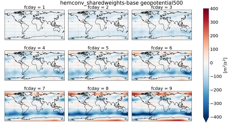
representing global data as rectangular images leads to strong distortions close to the poles. Here
we test a technique that circumvents this problem, and show that it increases forecast performance.
Additionally, we design our machine learning method in such a way that it “knows” a-priori that the
weather on the Earth’s two hemispheres is similar but "mirrored".

1     Introduction
Weather forecasting has for decades been dominated by numerical models build on physical principles,
the so-called Numerical Weather Prediction Models (NWP). These models have seen a constant
increase in skill over time [Bauer et al., 2015]. Recently, however, there has been a surge of interest
in data-driven weather forecasting in the medium-range (~2-14 days ahead), especially using neural
networks [Scher, 2018, Scher and Messori, 2019b, Dueben and Bauer, 2018, Weyn et al., 2019, 2020,
Faranda et al., 2020, Scher and Messori, 2020]. A historic overview of paradigms in weather prediction,
is outlined in [Balaji, 2020]. Many of the recently proposed data-driven approaches use convolutional
neural networks (CNNs) [Scher, 2018, Scher and Messori, 2019b, Weyn et al., 2019] or a local network
that is shared across the domain [Dueben and Bauer, 2018]. What these methods have in common
is that they use global data on a regular lat-lon grid. This, however, leads to distortions, especially
close to the poles. However, a standard convolution or shared local architecture does not take this
into account since it uses a filter whose size is a fixed number of gridpoints (e.g. 3×3). Therefore, the
area that the filter sees is not the same close to the Equator and close to the poles. Weyn et al. [2020]
have proposed a solution to this problem via working on a different grid. Specifically, they regrid
the data to a “cubed sphere” consisting of 6 different regions. Then they use a standard convolution
operation on each side of the cubed sphere. Additionally, they do not share the weights of the filters
globally (as in the original architecture proposed by Scher [2018] and adapted to real world data by
Weyn et al. [2019]), but they use an independent convolution operation for the different sides of the
cubed sphere. The weights are shared only for the two polar parts of the cubed sphere, but then
“flipped” from one pole to the other to account for the different direction of rotation.
    In this paper, we present an alternative approach to incorporate the spherical nature of the Earth
into CNNs. We use a technique called spherical convolution, which has previously been proposed for
classification tasks on 360◦ -images [Coors et al., 2018]. Additionally, we test two different approaches
of including information of the hemispheres into our networks. All these approaches can be seen
as variantd of “informed machine learning” [von Rueden et al., 2020], in which prior knowledge is
included into the machine-learning pipeline. In our case, the prior knowledge is that the Earth
is spherical (in contrast to the regular data that we provide), and that the dynamics of the two
hemispheres are - to some extent- “flipped” relative to each other. This information is directly
encoded into the structure of the neural network.
    The aim of this paper is not to create the best data-driven weather forecasts, but rather to assess
the effect of two possible adaptions of earlier proposed methods, and to disentangle their individual
contributions to forecast skill. These methods are tested on reanalysis data from the Weatherbench
dataset [Rasp et al., 2020]. This is a dataset specifically designed for benchmarking machine-learning
based weather forecasts. We use the data at a resolution of up to 1.4 deg, which is higher than in

                                                    2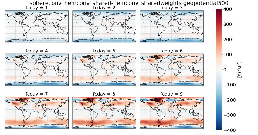
previous studies. We assess both medium range forecast skill and long-term stability of forecasts.
Finally, we include an analysis of the events with highest forecast errors. These are important from an
end-user point of view, and in NWP they have elicited significant attention models. The occurrence
of unusually bad forecasts (“forecast busts”) in NWP models is connected with certain weather
situations [Rodwell et al., 2013, Lillo and Parsons, 2017], and more generally, different weather
situations have different predictability [Ferranti et al., 2015]. We analyze whether the worst forecasts
of our data-driven forecasts systems are randomly distributed, or, as in NWP, are associated with
recurrent weather situations.

2     Methods
2.1    Data
We use data from Weatherbench Rasp et al. [2020], a benchmark dataset for data-driven weather
forecasting. The subset we use consists of ERA5 reanalysis data, regridded to a regular lat-lon grid
with two different resolutions: 2.8125 deg (hereafter called “low-resolution” or “lres”) and 1.40625
deg (hereafter called “high-resolution” or “hres). The following input variables are used: temperature
at 500 and 850 hPa, geopotential at 500 and 850 hPa. As evaluation variables, we use gepotential
height at 500hPa (“z500”) and temperature at 850hPa (“t850”). We use the period 1979-2016 for
training and validation, and 2017-2018 for evaluation (as proposed in Weatherbench).
    The forecasts of the network trained on the lres data are evaluated only on the lres grid. The
forecasts made with the hres architecture are evaluated both on the hres grid and, after bilinear
regridding, also on the lres grid.

2.2    Spherical convolution
In normal convolution, for each gridpoint, a fixed number of gridpoints in the vicinity are sampled
(for example a 3×3 box centered on the gridpoint). For data from a globe (such as global atmospheric
data) represented on a regular grid, this leads to distortions except very close to the equator. Indeed,
a fixed neighborhood defined via number of gridpoints corresponds to a rectangle of differing size,
depending on latitude. One way to remedy this is through the use of spherical convolution. Coors
et al. [2018] proposed spherical convolution in neural networks for image detection in spherical images.
Our method is based on this method, with a modification regarding the projection. The original
method was tailored for the gnomic projection. Since our data is on a regular grid, we changed the
interpolation accordingly.
    With this method, instead of a box of fixed size in gridpoint space, each gridpoint is assigned
a rectangle with fixed size in real space. Since the positions of available gridpoints and the target
coordinates in this fixed size box do not necessarily coincide, the target can also be an interpolation of
gridpoints. For general projections and general kernels, this could mean an interpolation between up
to four gridpoints. However, we use data on a regular grid, and allow only multiples of the gridpoint
distance at the equator as points in the latitude direction. Therefore, only longitude needs to be
interpolated, and each target point is a (linear) interpolation between two gridpoints. The principle

                                                    3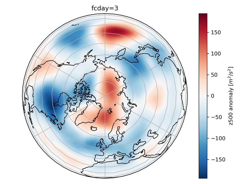
Z500, z850,
                                                                                                           sin(doy),cos(doy),
                                                                                        t500, t850
                                                                                                           sin(hod), cos(hod)
                                                                                       2 timesteps
                                                                                                               128x156x4
                                                                                        128x256x8

                                                                                                input 128x256x12

                                                                                         custom convolution 128x256x32

                                                                                         custom convolution 128x256x32

                                                                                         average pooling 64x128x32
                Standard kernel   Dense (“fractional”)
                                  kernel                                                custom convolution 64x128x64

                                                                                       custom convolution 64x128x64

                                                                                       average pooling 32x64x64

                                                                  Return output for
                                                                                      custom convolution 32x64x128

                                                                  second step
                                                                                      custom convolution 32x64x64
        N
                                                                                        upsampling 64x128x64
                                                                                          concatenate 64x128x128

                                                                                        custom convolution 64x128x64

                                                                                       custom convolution 64x128x32

                                                                                          upsampling 128x256x32
                                                                                             concatenate 64x128x64

                                                                                         custom convolution 128x256x32
        EQ                                                                               custom convolution 128x256x32

                                                                                      custom convolution (linear) 128x256x8

                                                                                               add 128x256x8

a)                                                           b)

Figure 1: a) Sketch of the principle of spherical convolution. Shown is a standard 3×3 kernel
(corresponding to 3×3 gridpoints at the equator), and a 3×5 “dense” kernel, covering the same area,
but with more detail. b) overview of neural network structure. Dimensions are for the hres data.

is sketched in fig. 1 a).
     In normal convolution operations in neural networks, the kernel is always made up of exact
gridpoints (e.g. a 3×3 corresponding to 9 gridpoints). Our approach requires interpolation, and thus
our method also allows the use of a non-integer number of gridpoints in the kernel. For example, we
can use the distances -1,-0.5,0,0.5,1 along the longitude direction, creating a kernel of 5 gridpoints,
corresponding to the distance of 3 gridpoints at the equator. This is shown in the right part of fig.
1 a). In principle this could also be implemented in the longitude direction, although we chose not
do this here.

2.2.1       Implementation

Since Coors et al. [2018] have not provided details on their technical implementation, and since their
code is not publicly available, we have designed our own implementation of spherical convolution. In
this section we use the word “tensor” as it is used in computational packages such as tensorflow, thus
interchangeably with “array”. Therefore, not everything referred to as a tensor here is necessarily a
tensor in the strict mathematical sense.
     We have implemented the spherical convolution in the following steps (the channel dimension of

                                                         4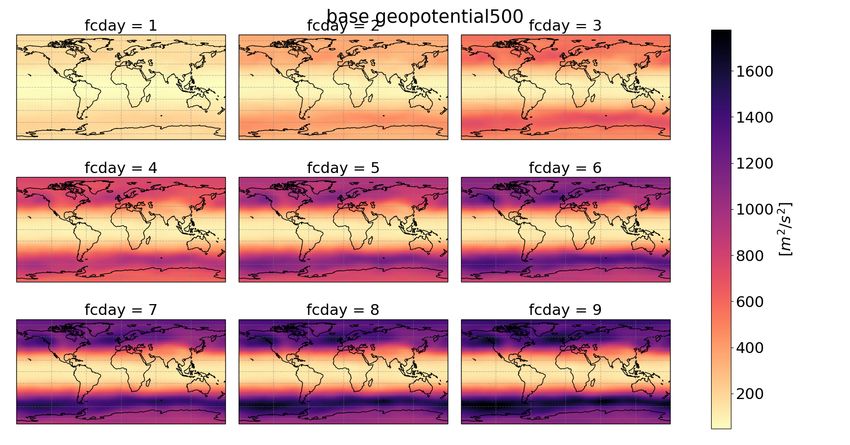
the neural network is omitted here for simplification):

  1. we start with a (fixed) filter kernel K
                                           ~ of length n, consisting of n pairs of lat-lon distances
      ∆pi = (∆yi , ∆xi ), corresponding to gridpoints at the equator. A 3×3 kernel without fractional
      distances for example would be
      [(−1, −1) , (−1, 0) , (−1, 1) , (0, −1) , (0, 0) , (0, 1) , (1, −1) , (1, 0) , (1, 1)].

  2. for each of the N × M input gridpoints p = (x, y) in the regular grid, we compute n pairs of
      (potentially non-integer) coordinates p0 = (yi0 , x0i ), corresponding to the n points in the kernel
      ~ transformed for the current position of p on the globe with the following equations:
      K,

                                                     y0     = y + ∆y                                  (1)
                                                     x0   =x+        ∆x
                                                                   cos(φ)                             (2)

      with latitude φ of the central point. The transformed coordinates are in regular lat-lon coor-
      dinates. The transformed coordinates for each gridpoint and kernel points are combined in a
      coordinate tensor  of shape N × M × n.

  3. the input ~x data is flattened to ~xf lat with shape L = N · M , and the coordinate tensor  is
      flattened to a tensor of shape L × n, with the coordinates transformed to flattened coordinates.

  4. a sparse interpolation tensor L̂ of size L × L is created, and filled with the target coordinates
      in such a way that multiplying the flattened input data ~xf lat with the interpolation tensor
      results in the expanded input data ~xexp = L̂~x with shape L × n. L̂ is implemented as a sparse
      tensorflow tensor. This implementation allows the use also on very large grids (large L), as
      only the non-zero components are kept in memory.

  5. on ~xexp , a standard 1-d convolution with kernel size n (as implemented in major neural network
      libraries such as tensorflow) can now be applied, resulting in ~xout with size L, which is then
      unflattened to shape N × M

The steps 1,2, and the computation of the interpolation tensor needs to be done only once (when
setting up the network). L̂ is stored in memory for all subsequent operations.
   At gridpoints close to the poles, kernel-points can “pass” through the pole. For these points, not
only the longitude, but also the latitude is adjusted. For example, on a 1x1 deg gid a kernel point
that without this adjustment would correspond to the impossible point 90.5N 0E will be set as 89.5N
180E. With this, the “polar problem” of regular grids is eliminated.

2.3    Neural network architecture.
We use a neural network architecture based on that proposed in Weyn et al. [2020], namely a U-net
architecture. Weyn et al. however do not use data on a regular grid, but on a cubed sphere, consisting
of several regular grids. In each of their convolution layers in the U-net, a standard convolution is
made separately for each region, without sharing weights between the regions. We use the same
architecture, but with each of their special convolution layers replaced by a standard convolution,

                                                            5
our spherical convolution and/or hemisphere-wise convolution (see below). The network structure is
shown in fig. 1 b). Our networks are implemented in tensorflow [Martín Abadi et al., 2015] using
the dataset api with tensorflow record files, resulting in a scaleable implementation that should also
scale to datasets with higher resolution than used here.
In addition to the input variables from ERA5 discussed in the data-section, day of the year
(“doy”) and hour of the day (“hod) are used as additional input variables. Since these are “circular”
variables, each of them is converted to two variables:
2π
doy1 = sin doy (3)
365
2π
doy2 = cos doy (4)
365
2π
hod1 = sin doy (5)
24
2π
hod2 = cos doy (6)
24
These 4 scalars are extended to the grid-resolution of the data and added as additional channels.
The input of the networks is comprised of two timesteps (2 variables at 2 pressure levels each), but the
additional 4 variables are provided only once, resulting in 8+4=12 input channels. The output of the
networks are 2 timesteps of the input variables, without the additional variables (thus 8 channels).
One forecast step is made of two consecutive passes through the network, via feeding the output back
to the input, resulting in a 24 hour forecast. For details see Weyn et al. [2020].
For consecutive forecasts (longer than 24 hours), hod is not updated, since each forecast step
is 24 hours. We also choose not to updated doy, since the forecast length of 10 days is very short
compared to seasonal variations. Only for the long-term stability experiment in section 3.4 doy is
updated with each consecutive forecast step.
2.3.1 Base architecture
Our base architecture without spherical convolution uses normal convolution. Along the longitude
direction the convolution is “wrapped” around, so there is no artificial boundary. At the poles the
grid is padded with zeros to make the output of the convolution operation the same size as the input.
This is the same approach for dealing with the boundaries as in Weyn et al. [2019]. The kernel size
of the convolutions is 3×3.
2.3.2 Spherical convolution architecture
The spherical convolution architecture is the same as the base architecture, except that each convo-
lution operation is replaced by a spherical convolution operation. Since the convolution deals both
with the poles and the longitude-wrap, no padding is applied. In the standard spherical convolution
architecture (“sphereconv”) we use a 3×3 kernel, just as in the base architecture. Additionally, we
test a second architecture with a 3×7 dense kernel. Here, in the longitude direction, the distance
6of 3 gridpoints at the equator is covered by 7 evenly spaced kernel points. This architecture will be
referred to as “spherconv_densekernel”, and is only tested on the lres data. This is motivated by the
poor performance on the lres data (see section 3).
2.3.3 Hemispheric convolution
We use two related approaches for incorporating the fact there there are 2 hemispheres into the net-
works. In the first, we use separate (independent) convolution operations (with separate weights) for
each hemisphere. The data is split at the equator. For the architecture without spherical convolution,
the first row of the other hemisphere is added as padding for the boundary of the convolution. When
using spherical convolution together with hemispheric convolution this is not necessary, as this is
included in the interpolation for the spherical convolution. Then, on each hemisphere, a convolution
operation is performed. This will be referred to as “hemconv” and “sphereconv_hemconv”. In the sec-
ond approach, the same convolution operation is used for both hemispheres, with the filter “flipped”
along the lat dimension for the second hemisphere. This will be referred to as “hemconv_shared”
and “sphereconv_hemconv_shared”. This approach is a variant of the inclusion of “invariances” into
the neural network in the terminology of von Rueden et al. [2020].
2.3.4 Training details
Each network is trained 5 times with different random seeds to account for the randomness in the
training. Each training realization is evaluated separately, and throughout the paper the average of
the errors and skill scores is shown. The same architecture is used both for high and low resolution
data. Only the input size is adjusted according to the resolution. Since the architecture is a pure
convolution architecture, the number of parameters (weights) is independent of the input size, and
thus both for hres and lres the same number of parameters is used (336,040 for architectures with
same weights for both hemispheres, and 671,816 for the architectures with independent weights for
each hemisphere). We train the networks first for 4 epochs (10 epochs for hres), and then over an
additional 50 (20 for hres) epochs with early stopping (stopping after no increase in skill at 10% of
the training data left out for validation). The reason for less epochs for the hres data was solely to
reduce computational time.
The data from Weatherbench is converted to the tensorflow-record format.
2.4 Forecast evaluation
We use both Root Mean Square Error (RMSE) and Anomaly Correlation Coefficient (ACC), which
are also the two measures used in Weatherbench.
RMSE is defined as
2
RM SE = (f c − truth) (7)
with the overbar representing latitude-weighted area and time mean,and ACC as
ACC = corr(f c − clim, truth − clim) (8)
7with the correlation computed with latitude weights and clim the time-mean over all forecasts.
For details of the calculations see Rasp et al. [2020].
3 Results
We start by looking at global average RMSE and ACC, shown in fig. 2-3 and table 1. The upper
panels of the figures show absolute values, whereas the lower panels show the difference to the
base architecture. The base architecture has the next to lowest skill at all lead times, with only
sphereconv_densekernel performing worse (sphereconv_densekernel is omitted from the difference
panels in order to better visualize the difference between the other architectures). Sphereconv does
consistently better than the base architecture. This holds for all lead-times, both resolutions and both
for RMSE and ACC, except for day 1 on the lres data, where sphereconv is slightly worse than base.
The improvement is however relatively small. Changing the kernel of the spherical convolution to
the densekernel (higher kernel resolution in the latitude direction) degrades forecast skill to far below
even the base architecture. Due to this negative result we decide not to test the (computationally
expensive) dense kernel method on the high resolution data.
The hemconv architecture is better than the base architecture, and mostly also better than
than the sphereconv architecture on the hres data, but on the lres data it is slightly worse than
sphereconv at most lead times. The hemisphere convolution architecture with shared (flipped) weights
(hemconv_shared) outperforms the hemisphere convolution architecture with independent weights.
The same holds when combining spherical convolution with hemisphere-wise convolution. Both
hemisphere methods lead to an additional improvement on top of the spherical convolution, but
sharing the flipped weights leads to the best result. The architecture with spherical convolution
and hemispheric convolution with shared weights (sphereconv_hemconv_shared) is the best of all
architectures on lres for all lead-times, and on hres up to day 4, with roughly equal contributions
from the spherical convolution and from the splitting into hemispheres.
Evaluating the hres forecasts on the lres grid instead of on the hres grid has only a small influence,
with slightly lower errors than when evaluating on the hres data, but not changing the basic results
(table 1).
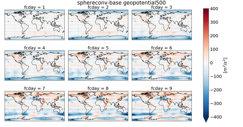
We now turn to the spatial distribution of RMSE for z500 (fig. 4). Panel a) shows the error of
the base networks at different lead times for the hres data, with increasing leadtime from upper left
to lower right. The error pattern follows the typical error patterns of medium range NWP forecasts,
with lowest predictability in the storm-track regions (e.g. Scher and Messori [2019a]). As expected,
the error grows with increasing lead-time, with no dramatic changes in the spatial patterns.
More interesting is the difference between the spherconv and the base architecture (panel b) and
the difference between sphereconv_hemconv_shared and hemconv_shared (panel d). Up to forecast
day 4, the spherical convolution clearly improves the forecasts around both poles. In the Northern
Hemisphere, however, the spherconv forecasts in the storm track regions are slightly worse than the
base architecture, and for longer lead-times also the forecasts around the North Pole are worse with
the spherical convolution. Results are similar for t850 (fig. S1), except that for t850 hres the longer
forecasts around the north pole have the same error both in the base architecture and the spherconv
8geopotential 500 day 3/5 [m2/s2] temperature 850 day 3/5 [K]
hres base 575 / 863 2.88 / 3.92
hres sphereconv 558 / 836 2.82 / 3.84
hres hemconv 549 / 825 2.80 / 3.86
hres hemconv_shared 516 / 781 2.71 / 3.74
hres sphereconv_hemconv 525 / 818 2.76 / 3.87
hres sphereconv_hemconv_shared 496 / 800 2.68 / 3.79
hres base regrid 572 / 859 2.8 / 3.85
hres sphereconv regrid 555 / 832 2.74 / 3.78
hres hemconv regrid 545 / 820 2.73 / 3.8
hres hemconv_shared regrid 512 / 777 2.63 / 3.68
hres sphereconv_hemconv regrid 522 / 814 2.68 / 3.81
hres sphereconv_hemconv_shared regrid 492 / 796 2.61 / 3.73
lres base 539 / 834 2.8 / 3.87
lres sphereconv 527 / 803 2.75 / 3.8
lres hemconv 526 / 816 2.77 / 3.86
lres hemconv_shared 501 / 795 2.66 / 3.75
lres sphereconv_hemconv 502 / 782 2.74 / 3.82
lres sphereconv_hemconv_shared 454 / 734 2.61 / 3.69
sphereconv_denskernel 687 / 1043 3.5 / 5.05
IFS T42 489 / 743 3.09 / 3.83
IFS T63 268 / 463 1.85 / 2.52
Operational IFS 154 / 334 1.36 / 2.03
Table 1: Baseline scores (RMSE) on the Weatherbench dataset, including NWP model scores as
baselines.
architecture.
Finally, panel c) compares hemconv_shared with the base architecture. Here the improvements
in the first days of the forecasts are more spatially uniform.. Interestingly, from day 5 onward
there is a deterioration around both poles in the hemconv_shared architecture compared to the base
architecture.
3.1 Long term stability
We next assess the long-term stability of forecasts for lead-times beyond 10 days. For this, we start
a forecast from a date in January 2017 and perform iterative forecasts for a whole year. The doy
input is updated every day to account for the seasonality. This is repeated with several January
dates from 2017. The result for one starting date and one training realization is shown in fig. 5. The
figure shows z500 of the 1-year forecast made by the sphereconv_shared architecture (panel a), of
the hemconv_shared architecture (panel b) and the corresponding analysis from ERA5 (panel c). As
can be seen, the yearly cycle of the forecast is highly unrealistic. This is the same for other starting
dates (not shown). Additionally, some training realizations produce even more unrealistic long-term
forecasts (not shown). This might indicate that the doy as boundary condition is not sufficient to
reproduce a good yearly cycle, and/or that the networks introduce substantial non-physical errors
that accumulate over time.
9a) b)
d)
c)
Figure 2: Forecast skill (RMSE and ACC) for all hres (1.4◦ ) architectures for geopotential at 500hPa
and temperature at 850hpa. a,b: absolute values, c,d: difference to base architecture.
10a) b) h
d)
c)
Figure 3: Forecast skill (RMSE and ACC) for all lres (2.8◦ ) architectures for geopotential at
500hPa and temperature at 850hpa. a,b: absolute values, c,d: difference to base architecture. In c,d
sphereconv_densekernel is ommited in order to be able to better visualize the differences between
the other methods.
11a) b)
c) d)
Figure 4: a): RMSE of geopotential at 500 hpa [m2 /s2 ] of the base architecture. b) difference in
RMSE between sphereconv and base c) difference between hemconv_shared and base d) difference
between sphereconv_hemvonc_shared and hemconv_shared
3.2 Analysis of events with highest errors
We now look at the forecasts within the upper 5% of RMSE (forecast “busts”) for the Northern
Hemisphere (NH) for lead-time 3 for the spherconv_hemconv_shared architecture (the architecture
with highest forecast skill in the first days of the forecast). For each of the 5 training realizations, the
percentile is computed individually. When comparing the initialization dates of the worst forecasts,
~20% are exactly the same dates for all members, ~36% occur in at least 4 of the 5 members, ~50%
in at least 3 of the 5 members (fig. 6 a). This is much higher than expected by chance if the events
were randomly distributed. Events with high error are more common in winter than in summer (fig.
6 b), in line with the performance of operational NWP models.
Finally, fig. 6 b) shows a composite of z500 anomaly of all initial times at which at least one of the
spherconv_hemconv hres networks had an error > 95% in the NH. The anomaly is computed with
respect to the mean over 2016-2017 (the evaluation period), and separately for each month. There are
positive anomalies east of Greenland and in the middle of the Northern Pacific, and (less pronounced)
negative anomalies over northern Canada, the eastern coast of Asia and over central Europe. These
results are similar for other architectures (fig. S2-S4), and for other lead-times (fig. S5-S8). This
indicates that the skill of the network forecasts is dependent on the atmospheric configuration, just
as in NWP forecasts (e.g. Ferranti et al. [2015]).
3.3 Computational Performance
Replacing standard convolution with spherical convolution introduces a significant amount of addi-
tional computations. While the use of sparse tensorflow tensors for the interpolation tensor L̂ avoids
12a) b)
c)
Figure 5: Evolution of a single long term forecast for hemconv_shared (a) and sphere-
conv_hemconv_shared (b), and verifying reality (c). Everything 500hpa geopotential.
13a) b)
c)
Figure 6: a) fraction of dates with extreme forecast error (>95%) that occur in at least n_common
out of 5 members for sphereconv_hemconv_shared. b) yearly cycle of dates with at least one member
with extreme forecast error. All forecasts day 3 with hres data. c) composite mean of z500 of all days
where at least 1 member has a bust, shown as anomaly with respect to deseasonalized time mean of
2016-2018.
14large memory requirements, the computation time of the sphereconv network for the hres datacom-
pared to the base architecture is roughly a factor 6 higher on a CPU with 2 cores (14 vs 2.4s),
and by a factor of 20 higher on a NVIDIA Tesla v100 GPU (1.0s vs 50ms). Using hemisphere-wise
convolution does not introduce any significant performance overhead (with shared weights ~4%, with
separate weights none at all).
4 Discussion and Conclusion
In this paper we have tested two approaches to improve data-driven weather forecasts with CNNs.
Firstly, we have tested replacing standard convolution operations with exact spherical convolution.
Secondly, we tested integrating basic meteorological knowledge into the structure of the networks,
namely that the dynamic of one hemisphere is “flipped” with respect to the other hemisphere. This we
have hardcoded into our networks via flipping the weights of the network. In a variant of this method,
we have also used independent weights for each hemisphere. These methods (and combinations of
them) were tested on the ERA5 data from the Weatherbench dataset [Rasp et al., 2020]. We used
a neural network architecture previously proposed by Weyn et al. [2020], and adapted it to our
convolution methods. We found that both the spherical convolution and the hemisphere-information
improve the forecasts, but in different ways. Spherical convolution mainly leads to improvements
close to the poles, and less so in other regions. The hemisphere-specific information instead leads
to relatively uniform improvements in the mid-latitudes, where the largest forecast errors appear.
For the first couple of days, combining spherical convolution with hemisphere-wise convolution with
shared flipped weights leads to the best forecasts. Compared to the base architecture, spherical
convolution and hemisphere-wise convolution contribute roughly equally to forecast improvement.
Finally, we have found that initial conditions causing largest forecast errors are relatively consis-
tent across different training realizations of the same network. This indicates, as one would expect,
that errors of neural network weather forecasts are not completely random, but controlled at least
partly by the intrinsic predictability of the atmospheric state (and by the error in the used analysis
product).
Our approach innovates over previous studies in the field in several respects. Weyn et al. [2020]
have split up the world into a couple of regions, with each region being represented by a local grid. On
these local grids they used standard convolution operations. This method still leads to distortions, as
even a subregion of the Earth’s surface cannot be represented on a local regular grid with complete
accuracy. In addition, this method also needs padding, which at the edges is ambiguous. Weyn
et al. [2020] have only tested a configuration where the weights are not shared between the different
regions (except between the two polar regions, where they use the same but “flipped” weights for
the second pole). Therefore, it is not possible to disentangle the effect of local convolutions and the
effect of dealing with the spherical nature of the Earth. Finally, Weyn et al. [2020] have used different
input variables (for example they have included radiation as well), which might explain their higher
skill and long-term stability compared to the results here. From a practical point of view, there are
also differences. The method of Weyn et al. needs data-preprocessing (regridding), but then can
use standard neural network operations. In our approach, the standard data can be used, but the
15spherical convolution introduces computational overhead in every pass through the network.
The fact that the additional relative runtime needed for the networks with spherical convolution
is higher on a GPU than on CPU could indicate that the implementation using sparse tensorflow
tensors is not optimized for GPUs. For small input sizes, an alternative would be to use standard
tensorflow tensors (still filled sparsely, but represented as a full tensor (array) in memory), but for
full resolution ERA5 data (0.25 deg resolution, 3600x1801 gridpoints on a regular latlon point) this
would not be feasible with current computers due to memory limitations, since the interpolation
tensor then has a size of 6483600x6483600.
The aim of our study was not to provide the best possible neural network based weather forecasts,
but to assess the effect of two specific changes to a neural network architecture. Still, possible
improvements to the methods presented here could be:
• splitting up the convolution for smaller different regions (similar to Weyn et al. [2020])
• including locally connected layers (here each gridpoint in a layer is also a combination of the
inputs from a certain kernel (e.g. 3×3), but the weights are not shared across the domain.
• adding more prior information into the structure of the network, for example vertical structure
of the atmosphere.
Acknowledgements
The computations were enabled by resources provided by the Swedish National Infrastructure for
Computing (SNIC) at National Supercomputer Centre (NSC) and High Performance Computing
Center North (HPC2N) partially funded by the Swedish Research Council through grant agreement
no. 2018-05973.
Author contributions
S.S. designed and implemented the methods of the paper and drafted the manuscript. Both authors
discussed and interpreted the results and improved the manuscript.
References
V. Balaji. Climbing down Charney’s ladder: Machine Learning and the post-Dennard era of compu-
tational climate science. arXiv:2005.11862 [nlin, physics:physics], May 2020.
Peter Bauer, Alan Thorpe, and Gilbert Brunet. The quiet revolution of numerical weather prediction.
Nature, 525(7567):47–55, September 2015. ISSN 1476-4687. doi: 10.1038/nature14956.
Benjamin Coors, Alexandru Paul Condurache, and Andreas Geiger. SphereNet: Learning Spherical
Representations for Detection and Classification in Omnidirectional Images. In Vittorio Ferrari,
Martial Hebert, Cristian Sminchisescu, and Yair Weiss, editors, Computer Vision – ECCV 2018,
Lecture Notes in Computer Science, pages 525–541, Cham, 2018. Springer International Publishing.
ISBN 978-3-030-01240-3.
16Peter D. Dueben and Peter Bauer. Challenges and design choices for global weather and climate
models based on machine learning. Geoscientific Model Development, 11(10):3999–4009, October
2018. ISSN 1991-959X. doi: 10.5194/gmd-11-3999-2018.
Davide Faranda, M. Vrac, P. Yiou, F. M. E. Pons, A Hamid, G Carella, C. G. Ngoungue Langue,
S. Thao, and V. Gautard. Boosting performance in machine learning of geophysical flows via scale
separation. June 2020.
Laura Ferranti, Susanna Corti, and Martin Janousek. Flow-dependent verification of the ECMWF
ensemble over the Euro-Atlantic sector. Quarterly Journal of the Royal Meteorological Society, 141
(688):916–924, April 2015. ISSN 1477-870X. doi: 10.1002/qj.2411.
Samuel P. Lillo and David B. Parsons. Investigating the dynamics of error growth in ECMWF
medium-range forecast busts. Quarterly Journal of the Royal Meteorological Society, 143(704):
1211–1226, 2017. ISSN 1477-870X. doi: 10.1002/qj.2938.
Martín Abadi, Ashish Agarwal, Paul Barham, Eugene Brevdo, Zhifeng Chen, Craig Citro, Greg S.
Corrado, Andy Davis, Jeffrey Dean, Matthieu Devin, Sanjay Ghemawat, Ian Goodfellow, Andrew
Harp, Geoffrey Irving, Michael Isard, Yangqing Jia, Rafal Jozefowicz, Lukasz Kaiser, Manjunath
Kudlur, Josh Levenberg, Dandelion Mané, Rajat Monga, Sherry Moore, Derek Murray, Chris Olah,
Mike Schuster, Jonathon Shlens, Benoit Steiner, Ilya Sutskever, Kunal Talwar, Paul Tucker, Vin-
cent Vanhoucke, Vijay Vasudevan, Fernanda Viégas, Oriol Vinyals, Pete Warden, Martin Watten-
berg, Martin Wicke, Yuan Yu, and Xiaoqiang Zheng. TensorFlow: Large-Scale Machine Learning
on Heterogeneous Systems. 2015.
Stephan Rasp, Peter D. Dueben, Sebastian Scher, Jonathan A. Weyn, Soukayna Mouatadid,
and Nils Thuerey. WeatherBench: A benchmark dataset for data-driven weather forecasting.
arXiv:2002.00469 [physics, stat], June 2020.
Mark J. Rodwell, Linus Magnusson, Peter Bauer, Peter Bechtold, Massimo Bonavita, Carla Cardi-
nali, Michail Diamantakis, Paul Earnshaw, Antonio Garcia-Mendez, Lars Isaksen, Erland Källén,
Daniel Klocke, Philippe Lopez, Tony McNally, Anders Persson, Fernando Prates, and Nils Wedi.
Characteristics of Occasional Poor Medium-Range Weather Forecasts for Europe. Bulletin of
the American Meteorological Society, 94(9):1393–1405, September 2013. ISSN 0003-0007. doi:
10.1175/BAMS-D-12-00099.1.
S. Scher. Toward Data-Driven Weather and Climate Forecasting: Approximating a Simple General
Circulation Model With Deep Learning. Geophysical Research Letters, 0(0), November 2018. ISSN
0094-8276. doi: 10.1029/2018GL080704.
S. Scher and G. Messori. How Global Warming Changes the Difficulty of Synoptic Weather
Forecasting. Geophysical Research Letters, 46(5):2931–2939, 2019a. ISSN 1944-8007. doi:
10.1029/2018GL081856.
Sebastian Scher and Gabriele Messori. Weather and climate forecasting with neural networks: Using
GCMs with different complexity as study-ground. Geoscientific Model Development Discussions,
pages 1–15, March 2019b. ISSN 1991-959X. doi: 10.5194/gmd-2019-53.
17Sebastian Scher and Gabriele Messori. Ensemble neural network forecasts with singular value de-
composition. arXiv:2002.05398 [physics], February 2020.
Laura von Rueden, Sebastian Mayer, Katharina Beckh, Bogdan Georgiev, Sven Giesselbach, Raoul
Heese, Birgit Kirsch, Julius Pfrommer, Annika Pick, Rajkumar Ramamurthy, Michal Walczak,
Jochen Garcke, Christian Bauckhage, and Jannis Schuecker. Informed Machine Learning – A
Taxonomy and Survey of Integrating Knowledge into Learning Systems. arXiv:1903.12394 [cs,
stat], February 2020.
Jonathan A Weyn, Dale R Durran, and Rich Caruana. Can Machines Learn to Predict Weather?
Using Deep Learning to Predict Gridded 500-hPa Geopotential Height From Historical Weather
Data. Journal of Advances in Modeling Earth Systems, 2019.
Jonathan A. Weyn, Dale Richard Durran, and Rich Caruana. Improving data-driven
global weather prediction using deep convolutional neural networks on a cubed sphere.
http://www.essoar.org/doi/10.1002/essoar.10502543.1, March 2020.
18You can also read