Interpretable Neuron Structuring with Graph Spectral Regularization
←
→
Page content transcription
If your browser does not render page correctly, please read the page content below
Interpretable Neuron Structuring with
                                                               Graph Spectral Regularization

                                               Alexander Tong ∗                     David van Dijk ∗                 Jay S. Stanley III
                                              Dept. of Comp. Sci.            Dept. of Genetics & Comp. Sci.      Comp. Bio. & Bioinfo. Prog.
                                                Yale University                      Yale University                  Yale University
arXiv:1810.00424v4 [cs.LG] 27 May 2019

                                             New Haven, CT, USA                  New Haven, CT, USA                New Haven, CT, USA

                                                     Matthew Amodio                      Kristina Yim                 Rebecca Muhle
                                                     Dept. of Comp. Sci.               Dept. of Genetics             Dept. of Genetics
                                                       Yale University                  Yale University               Yale University
                                                    New Haven, CT, USA                New Haven, CT, USA            New Haven, CT, USA

                                                   James Noonan                      Guy Wolf †               Smita Krishnaswamy†
                                                  Dept. of Genetics            Dept. of Math. and Stat.     Depts. of Genetics & Comp. Sci.
                                                   Yale University             Université de Montréal               Yale University
                                                 New Haven, CT, USA            Montreal, QC, Canada              New Haven, CT, USA

                                                                                          Abstract

                                                      While neural networks have been used to classify or embed data into lower dimen-
                                                      sional spaces, they are often regarded as black boxes with uninterpretable features.
                                                      Here we propose Graph Spectral Regularization for making hidden layers more
                                                      interpretable without significantly affecting the performance of their primary task.
                                                      Taking inspiration from spatial organization and localization of neuron activations
                                                      in biological networks, we use a graph Laplacian that encourages activations to
                                                      be smooth either on a predetermined graph or on a feature-space graph learned
                                                      from the data via co-activations of a hidden layer of the neural network. We show
                                                      numerous uses for this including cluster indication and visualization in biological
                                                      and image data sets.

                                         1       Introduction

                                         Common intuitions and motivating explanations for the success of deep learning approaches rely
                                         on analogies between artificial and biological neural networks, and the mechanism they used for
                                         processing information. However, one aspect that is all but overlooked is the spatial organization of
                                         neurons in the brain. Indeed, the hierarchical spatial organization of neurons, determined via fMRI
                                         and other technologies [20, 16], is often leveraged in neuroscience works to explore, understand, and
                                         interpret various neural processing mechanisms and high level brain functions. In artificial neural
                                         networks (ANN), on the other hand, hidden layers offer no organization that can be regarded as
                                         equivalent to the biological one. This lack of organization poses great difficulties on exploring and
                                         interpreting the internal data representations provided by hidden layers of ANNs and the information
                                         encoded by them. This challenge, in turn, gives rise to the common treatment of ANNs as black
                                         boxes whose operation and data processing mechanisms cannot be easily understood. To address
                                             ∗
                                                 These authors contributed equally
                                             †
                                                 These authors contributed equally;   Corresponding author: smita.krishnaswamy@yale.edu

                                         Preprint. Under review.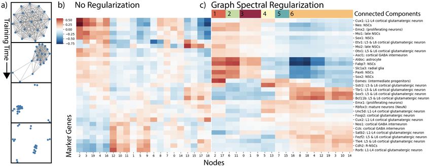
this issue, we focus on the problem of modifying ANNs to learn more interpretable feature spaces
without degrading their primary task performance.
While most neural networks are treated as black boxes, we note that there are methods in ANN
literature for understanding the activations of filters in convolutional neural networks (CNNs) [14],
either by examining trained networks [28], or by learning a better representation [15, 29, 21, 26, 22],
but such methods rarely apply to other types of networks, in particular dense neural networks (DNNs)
where a single activation is often not interpretable on its own. Furthermore, convolutions only apply to
datatypes where we know the feature structure apriori, as in the case of images and natural language.
In layers of a DNN, there is no enforced structure between neurons. The correspondence between
neurons and concepts is only determined based on the random initialization of the network. In this
work, we therefore encourage structure between neurons in the same layer, creating more localized
and interpretable layers.
More specifically we propose a Graph Spectral Regularization to encourage arbitrary graph structure
between neurons within a layer. The internal layers of a neural network are constrained to take the
structure of a graph, i.e. with graph neighbors activating on similar inputs. This allows us to map
the activations of a given layer over the graph, and interpret new input by examining the activations.
We show that graph-structuring a hidden layer causes useful, interpretable features to emerge. For
instance, we show that grid-structuring a layer of a classification network creates a structure over
which convolution can be applied, and local receptive fields can be traced to understand classification
decisions.
While a majority of the time imposing a known graph structure gives in interpretable results, there
are circumstances where we would like to learn the graph structure from data. In such cases we
can learn and emphasize the natural graph structure of the feature space. We do this by an iterative
process of encoding the data, and modifying the graph based on the feature co-activation patterns.
This procedure reinforces existing patterns in the data. This allows us to learn an abstracted graph
structure of features in high-dimensional realms such as single-cell RNA sequencing.
The main contributions of this manuscript are as follows: (1) Demonstration of hierarchical, spatial,
and smoothed feature maps for interpretability in dense networks. (2) A novel method for learning
and reinforcing the natural graph structure for complex feature spaces. (3) Demonstration of graph
learning and abstraction on single-cell RNA-sequencing data.

2   Related Work

CNN Interpretability: Unsurprisingly, most work focuses on the fully supervised classification
setting. Liao et al. [15] learned clustered CNN representations using a clustering regularization
showing better generalization, and stability, however cannot incorporate more general structures.
Jacobsen et al. [11] used convolutions along the feature dimension for hierarchical structure showing
fewer parameters were needed on the CIFAR dataset for the same accuracy with this architecture, but
did not examine any interpretability benefits. Sabour et al. [22] proposed a capsule representation,
where each capsule represents a group of neurons that encode a single meaning. In this work we
focus on a more general regularization that can encourage a wide range of intra-layer node structures.

Disentangled Representation Learning: While there is no precise definition of what makes for a
disentangled representation, the aim is to learn a representation that axis aligns with the generative
factors of the data [10, 2]. Higgins et al. [9] suggest a way to disentangle the representation
of variational autoencoders [13] with β-VAE. Subsequent work has generalized this to discrete
representations [5], and simple hierarchical representations [6]. These works focus on learning a
single vector representation of the data, where each element represents a single concept. In contrast,
our work learns a representation where groups of neurons may be involved in representing a single
concept. Moreover, disentangled representation learning can only be applied to unsupervised models
and only the most compressed level of either an autoencoder [9] or generative adversarial network as
in [4], whereas graph spectral regularization (GSR) can be applied to any or all layers of the network.

Graph Structure in ANNs: Graph based penalties have been used in the graph signal processing
literature [see e.g. 3, 30, 25], but are rarely used in an ANN setting. In the biological data setting, Min
et al. [18] used a graph penalty in sparse logistic regression on gene expression data. Another way of

                                                    2
utilizing graph structure is through Graph Neural Networks (GNN). GNNs are a related body of work
introduced by [8], and expanded on by [23], but focus on a different set of problems (For an overview
see [27]). We focus on learning a graph representation of general data while graph neural networks
only apply to data that comes as signals on a predefined feature graph. Although recent work by
Franceschi et al. [7] attempts to learn a model over the edges of the feature graph for a classification
task. This graph may be extremely large in high dimensional datasets, scaling quadratically with the
dimension, and we believe may be better learned in a lower dimensional representation.

3     Enforcing Graph Structure

In this paper, we consider the intra-layer relationships between neurons or larger structures such
as capsules as a graph. For a given layer of neurons we construct a graph G = (V, E) with
V = {v1 , . . . , vN } the set of vertices and E ⊆ V × V the set of edges. Let W be the weighted
symmetric adjacency matrix of size N × N with Wij = Wji ≥ 0 representing the weightPof the edge
between vi and vj . The graph Laplacian L is then defined as L = D − W where Dii = j Wij and
Dij = 0 for i 6= j.
To enforce smoothing we use the Laplacian smoothing loss on activation vector on some activation
vector z and fixed Laplacian L we formulate the graph spectral regularization function G as:
                                                  X
                              G(z, L) = z T Lz =      Wij ||zi − zj ||                       (1)
                                                        ij

We add it to the reconstruction or classification loss with a weighting term α. This adds an additional
objective that activations should be smooth along the graph defined by L. This optimization procedure
applies to any multi-layer model and valid graph Laplacian. We apply this algorithm to grid, and
hierarchical graph structures on both autoencoder and classification architectures.
Our method can be used to increase interpretability without much loss in representation power. At low
levels, GSR can be thought of as rearranging the activations so that they become spatially coherent.
As with other interpretability methods, GSR is not meant to increase representation power, but create
useful representations with low cost in power. Since GSR does not require an information bottleneck
such as in β-VAE, a GSR layer can be very wide, while still being interpretable. In comparing loss
of representation power, GSR should be compared to other regularization methods, namely L1 and
L2 penalties (See Table 1). In all three cases we can see that a higher penalty reduces the model
capacity. GSR affects performance in approximately the same way as L1 and L2 regularizations do.
To confirm this, we ran a MNIST classifier and measured train and test accuracy with 10 replicates.

                 Regularization Training accuracy Test Accuracy Coefficient
                          None 99.1 ± 0.3                 97.5 ± 0.3            N/A
                             L1 98.9 ± 0.3                97.4 ± 0.4            10−4
                             L2 98.3 ± 0.3                98.0 ± 0.2            10−4
                    GSR (ours) 99.3 ± 0.3                 98.0 ± 0.3            10−3
Table 1: MNIST classification training and test accuracies for coefficient selected using cross
validation over regularization weights in [10−7 , 10−6 , . . . , 10−2 ] for various regularization methods
with standard deviation over 10 replicates.

3.1   Computational Cost

Graph spectral regularization adds a bit more overhead than elementwise activation penalties. How-
ever, the added cost can be seen as containing one matrix vector operation per pass. Empirically, GSR
shows similar computational cost as other simple regularizations such as L1 and L2. To compare
costs, we used a Keras model with Tensorflow backend [1] on a Nvidia Titan X GPU and a dual
Intel(R) Xeon(R) CPU E5-2697 v4 @ 2.30GHz, and with batchsize 256. we observed during training
233 milliseconds (ms) per step with no regularization, 266ms for GSR, and 265ms for L2 penalties.

                                                    3
Algorithm 1 Graph Learning
    Input batches xi , model M with latent layer activations zi , regularization weight α.
    Pre-train M on xi with α = 0
    for i = 1 to T do
      Create Graph Laplacian Li from activations zi
      for j = 1 to m do
          Train M on xi with α = w and L = Li with MSE + loss in eq. 1
      end for
    end for

3.2    Learning and Reinforcing an Abstracted Feature-space Graph

Instead of enforcing smoothness over a fixed graph, we can learn a feature graph from the data (See
Algorithm 1) using neural network activations themselves to bootstrap the process. Note, that most
graph and kernel-based methods are applied over the space of observations but not over the space of
features. One of the reasons is because it is even more difficult to define a distance between features
than it is between observations. To circumvent this problem, we propose to learn a feature graph in
the latent space of a neural network using feature co-activations as a measure of similarity.
We proceed by creating a graph using feature activation similarity, then applying this graph using
Laplacian smoothing for a number of iterations. This converges to a graph of a latent feature space at
the level of granularity of the number of dimensions in the corresponding layer.
Our algorithm for learning the graph consists of two phases. First, a pretraining phase where the model
is learned with no graph regularization. Second, we alternate between constructing the graph from
the similarities of the embedding layer features and further training the network for reconstruction
and smoothness on the graph. There are many ways to create a graph from the feature × datapoint
activation matrix. We use an adaptive gaussian kernel,
                                          ||zi − zj ||22             ||zi − zj ||22

                                   1                         1
                      K(zi , zj ) = exp                    +   exp
                                   2           σi2           2            σj2
where σi is the adaptive bandwidth for node i which we set as the distance to the k th nearest neighbor
of feature. An adaptive bandwidth gaussian kernel is necessary as the scale of the activations is not
fixed in a standard neural network.
Since we are smoothing on the graph then constructing a new graph from the smoothed signal the
learned graph converges to a steady state where the mean squared error acts as a repulsive force to
stop the graph collapsing any further. We present the results of graph learning a biological dataset
and show that the learned structure adds interpretability to the activations.

4     Experiments
We present two examples of graph spectral regularization using standard graph structures, two where
we learn the underlying graph structure, and two where we represent hierarchical structure in the data.
Throughout, we show by visualizing the activations of data on the regularized layer, relationships
in the data that are not apparent in a standard neural network become clear. In learning the graph
structure we present two examples of high-dimensional biological datasets, and show that the learned
structure has biological relevance.

4.1    Fixed Structure

Enforcing fixed graph structure is a simple way to localize activations for similar datapoints. Here we
show that enforcing a simple 8x8 grid graph on a middle layer of a dense MNIST classifier causes
receptive fields to form, where each digit occupies a localized group of neurons on the grid. This can,
in principle, be applied to any neural network layer to group neurons activating to similar features.
Like in a real brain or convolutional neural network, we can examine the activation patterns for each
localized group of neurons. For a second example, we show the usefulness in encouraging localized
structure on a capsulenet architecture [22]. Where we are able to create globally consistent structure
for better alignment between capsules.

                                                   4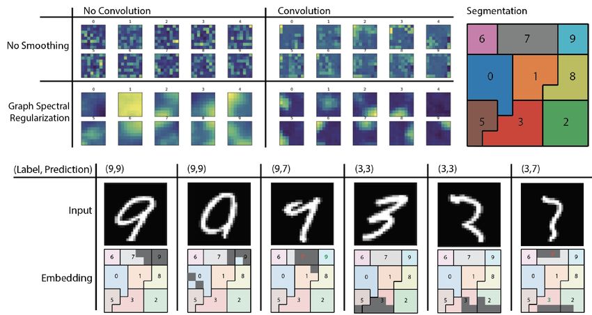
Figure 1: Shows average activation by digit over a 64 (8x8) 2D grid using graph spectral regularization
and convolutions following the regularization layer. Next, we segment the embedding space by class
to localize portions of the embedding associated with each class. Notice that the digit 4 here serves as
the null case and does not show up in the segmentation. Finally, we show the top 10% activation on
the embedding of some sample images. For two digits (9 and 3) we show a normal input, a correctly
classified but transitional input, and a misclassified input. By inspection of the embedding space we
can see the highlighted regions of the embedding space correlate with the semantic description of the
digit type.

Enforcing Grid Structure on Mnist We apply GSR to a classifier of MNIST digits. Without
GSR, activations are unstructured and as a result are difficult to interpret, in that it is difficult to
visually identify even which class a digit comes from based on the activation pattern (See Figure 1).
However, using GSR over a grid graph we can make this representation more visually distinguishable.
Since we can now take this embedding as an image, it is possible to use a standard convolutional
architecture in subsequent layers in order to further filter the encodings. When we add 3 layers of 3x3
2D convolutions with 2x2 max pooling we see that representations for each digit are compressed into
specific areas of the image. This leads to the formation of receptive fields over the network pertaining
to similar datapoints. Using these receptive fields, we can now extract the features responsible for
digit classification. For example, features that contribute to the activation of the top right of our grid
we can associate with those features that contribute to being the digit 9.
We show some correctly classified and incorrectly classified digits, in particular, we see that the
activation patterns on the embedding layer correspond well to a human perception of the digit type.
For example, the 9 that is misclassified as 7 both has significant activation in the 7 region of the
embedding layer, and looks visually close to a 7. We can now interpret the embedding layer as a sort
of brain map, where the map can map regions of activations, to types of inputs. This is not possible
in a standard neural network, where activations are not spatially organized.

Enforcing Node Consistency on Capsule Networks Here we use a capsule network consisting of
10 capsules of 16 nodes as in the original capsule network paper [22]. A capsule network represents
each digit as a 16 dimensional vector using a reconstruction penalty with a decoder. Sabour et al.
[22] notice that some of these 16 dimensions represent semantically meaningful differences in digit
representation such as digit scale, skew, and width. We train the same capsule net architecture
on MNIST with the graph spectral regularization applied between the matching ordinal nodes of
each capsule using fully connected graphs. We show in Figure 2 that in the standard capsule
network each capsule has its own ordering of features based on initialization However, with GSR
we obtain a consistent feature ordering, e.g. node 1 corresponds to line thickness across all digits.
For example, examine the line thickness feature. Line thickness is a global feature that is more

                                                    5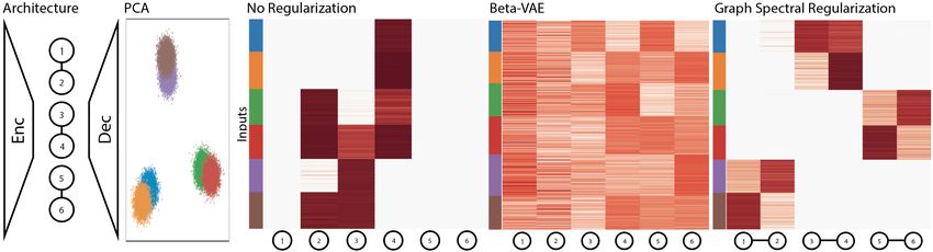
Figure 2: The prediction layer of a capsule network on MNIST uses 10 digit capsules each with 16
dimensions. To perform regularization between capsules we create 16 fully connected graphs of size
10. Next, we show dimension perturbations for each digit. Each column shows the reconstruction
when one of the 16 dimensions in the DigitCaps representation is tweaked by 0.05 in the interval
[-0.25, 0.25]. On the left we see a single dimension in a standard capsule net across all digits, and
on the right, we see a dimension on a capsule net trained with graph spectral regularization. With
graph spectral regularization between capsules (right) a single dimension represents line thickness
for all digits. Without this regularization each digit responds differently to perturbation of the same
dimension.
helpful for predicting reconstruction than classification, thus a line thickness feature can be globally
active across all capsules without diminishing classification performance. GSR can be thought of as
rearranging the capsule activations from a random ordering to a more interpretable ordering. GSR
does not degrade performance very much, as can be seen by the still excellent digit reconstructions
with GSR applied. GSR enforces a more ordered and interpretable encoding where localized regions
are similarly organized, and the global line thickness feature is consistently learned between digits.
More generally, GSR can be used to order nodes such that features common across capsules appear
together.
In these examples our goal was to enforce a data agnostic structure on unstructured features, but next
we will examine the case where we would like to investigate and learn the structure of the reduced
feature space.
4.2 Learning Graph Structure
When the graph is not defined apriori we can still extract meaningful structure by using the neural
network to learn a de novo graph from the data. As a sanity check, we first show that our method
can learn a simple cluster structure from the data. Then we apply this to a biological dataset that is a
trajectory rather than a cluster structure. Here our simple graph learning approach can learn structure
relevant to the overall structure in the data space.
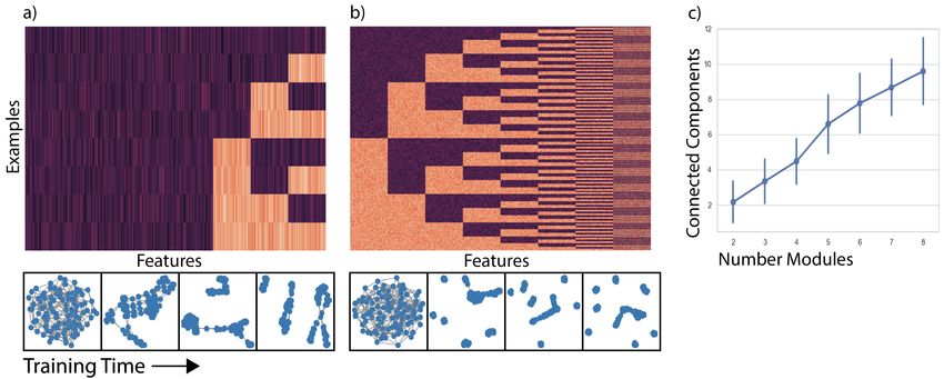
Extracting Structure on Ground Truth Dataset First, we learn a graph on a dataset constructed
with known feature structure to verify our method. We structure our nth dataset to have exactly n
modules. We generate the data with n modules by first creating 2n data points representing the binary
numbers from 0 to 2n − 1. In Figure 3 we can see both the structure of the data at three and eight
modules respectively, a plot showing the evolution of the latent graph over training time and a plot of
the number of modules in the data against the number of connected components in the learned graph.
The number of connected components is on average the number of modules therefore our graph
learning algorithm creates a data relevant graph. In the next example we show this graph learning
process on a natural dataset.
Extracting Trajectory Structure on T cell Development Data Next, we test graph learning on
biological mass cytometry data, which is a high dimensional, single-cell protein dataset, measured on
differentiating T cells from the Thymus [24]. The T cells lie along a bifurcating progression where
the cells eventually diverge into two lineages (CD4+ and CD8+). Here, the structure of the data is a
trajectory (as opposed to a pattern of clusters). We can see in Figure 4 how the activated nodes in
the graph embedding layer correspond to locations along the data trajectory. The activated nodes
(yellow) move from the bottom of the embedding to the top as T-cells develop into CD8+ cells. The
6Figure 3: We show the structure of the training data and snapshots of the learned graph for (a) three
modules and (b) eight modules. The number of modules should represent the number of graph
components in the final learned graph. In (c) we have the mean and 95% confidence interval of the
number of connected components in the trained graph for 50 trials run on each generated dataset.
Figure 4: Shows (a) graph structure over training iterations (b) feature activations of parts of the
trajectory. PHATE [19] plots colored by (c) branch number and (b) inferred trajectory location
showing the branching structure of the data.
CD4+ lineage is also CD8- and thus looks like a mixture between the CD8+ branch and the naive T
cells. The learned graph structure here has captured the transitioning structure of the underlying data.
4.3 Hierarchical Structure
Finally, we look at hierarchical structure, this is a very difficult structure for other interpretability
methods to learn, although recently specific methods look at this type of structure [6]. However, our
method naturally captures this by allowing for arbitrary graph structure among neurons in a layer.
First we show that if we would like to capture a structure known apriori, for example we are given
information that there are X distinct cell types, or X clusters in the data that we would like to examine
further, then we can do so by constructing the appropriate graph. If for example we know that there
should be 5 clusters of the data then we can form a graph with 5 disconnected complete subgraphs.
Finally, we show that we can learn this hierarchical structure in a developing neuron dataset without
prior knowledge on the number of clusters.
Enforcing Known Hierarchical Structure We demonstrate graph spectral regularization on data
that is generated with a hierarchical cluster structure. Our data contains three large-scale structures,
each comprising two Gaussian sub clusters generated in 15 dimensions (See Figure 5). We use this
dataset as it has both global and local structure. We demonstrate that our graph spectral regularized
model is able to pick up on both the global and local structure of this dataset where disentangling
methods such as β-VAE cannot. We use a graph-structure layer with six nodes with three connected
node pairs and employ the graph spectral regularization. After training, we find that each node pair
7Figure 5: Graph architecture, PCA plot, activation heatmaps of a standard autoencoder, β-VAE [9]
and a graph regularized autoencoder. In the model with graph spectral we are able to clearly decipher
the hierarchical structure of the data, whereas with the standard autoencoder or the β-VAE the
structure of the data is not clear.
acts as a “super node" that detects each large scale cluster. Within each super node, each of the two
nodes encodes one of each of the two Gaussian substructures. Thus, this specific graph topology is
able to extract the hierarchical topology of the data.
Figure 6: Shows correlation between a set of marker genes for specific cell types and embedding
layer activations. First with the standard autoencoder, then our autoencoder with graph spectral
regularization. The left heatmap is biclustered, the right heatmap is grouped by connected components
in the learned graph. We can see progression especially in the largest connected component where
features on the right of the component correspond to less developed neurons.
Extracting Hierarchical Cluster and Trajectory Structure on Single-cell RNA-Sequencing
Data In Figure 6 we learn a graph on a single-cell RNA-sequencing dataset of over 4000 cells
and over 8000 genes. The data contains a set of cells in the process of developing from neural stem
cells to full neurons in the mouse brain. While there are many gene modules that contribute to the
neuronal development, there are some states that have been studied. We use a list of cell type marker
genes to validate our method. We use 1000 PCA components of the data in an autoencoder with a 20
dimensional embedding space. We learn the graph using an adaptive bandwidth gaussian kernel with
the bandwidth for each feature set to the Euclidean distance to the nearest neighboring feature.
Our graph learns six components that represent meta features over the gene space. We can identify
each with a specific type of cell or related types of cells. For example, the light green component
(cluster 2) represents the very early stage neural stem cells as it is highly correlated with increased
Aldoc, Pax6 and Sox2 gene expression. Most interesting to examine is cluster 6, the largest component,
which represents development into mature neurons. Within this component we can see a progression
from just after intermediate progenitors on the left (showing Eomes expression) to more mature
neurons with higher expression of Tbr1 and Sox5. With a standard autoencoder we cannot see
progression structure of this dataset. While some of the more global structure is captured, we fail to
see the data progression from intermediate progenitors to mature neurons. Learning a graph allows
8us to create receptive fields e.g. clusters of neurons that correspond to specific structures within the
data, in this case cell types. Within these neighborhoods, we can pick up on the substructure within a
single cell type, i.e. their developmental trajectory.
5 Conclusion
We have introduced a novel biologically inspired method for regularizing features of the internal
layers of dense neural networks to take the shape of a graph. We show that coherent features emerge
and can be used to interpret the underlying structure of the dataset. Furthermore, when the intended
graph is not known apriori, we have presented a method for learning the graph structure, which learns
a graph relevant to the data. This regularization framework takes a step towards more interpretable,
accurate neural networks, and has broad applicability for future work seeking to reveal important
structure in real-world biological datasets as we have demonstrated here.
References
[1] Abadi, M., Barham, P., Chen, J., Chen, Z., Davis, A., Dean, J., Devin, M., Ghemawat, S., Irving,
G., Isard, M., Kudlur, M., Levenberg, J., Monga, R., Moore, S., Murray, D. G., Steiner, B.,
Tucker, P., Vasudevan, V., Warden, P., Wicke, M., Yu, Y., and Zheng, X. TensorFlow: A system
for large-scale machine learning. OSDI, pp. 21, 2016.
[2] Achille, A. and Soatto, S. Emergence of Invariance and Disentanglement in Deep Representa-
tions. arXiv:1706.01350 [cs, stat], June 2017.
[3] Belkin, M., Matveeva, I., and Niyogi, P. Regularization and semi-supervised learning on large
graphs. In International Conference on Computational Learning Theory, pp. 624–638. Springer,
2004.
[4] Chen, X., Duan, Y., Houthooft, R., Schulman, J., Sutskever, I., and Abbeel, P. InfoGAN:
Interpretable Representation Learning by Information Maximizing Generative Adversarial Nets.
arXiv:1606.03657 [cs, stat], June 2016.
[5] Dupont, E. Learning Disentangled Joint Continuous and Discrete Representations. In Bengio, S.,
Wallach, H., Larochelle, H., Grauman, K., Cesa-Bianchi, N., and Garnett, R. (eds.), Advances
in Neural Information Processing Systems 31, pp. 710–720. Curran Associates, Inc., 2018.
[6] Esmaeili, B., Wu, H., Jain, S., Bozkurt, A., Siddharth, N., Paige, B., and Brooks, D. H.
Structured Disentangled Representations. AISTATS, pp. 10, 2019.
[7] Franceschi, L., Niepert, M., Pontil, M., and He, X. Learning Discrete Structures for Graph
Neural Networks. arXiv:1903.11960 [cs, stat], March 2019.
[8] Gori, M., Monfardini, G., and Scarselli, F. A new model for learning in graph domains. In
Proceedings. 2005 IEEE International Joint Conference on Neural Networks, 2005., volume 2,
pp. 729–734, Montreal, Que., Canada, 2005. IEEE. ISBN 978-0-7803-9048-5. doi: 10.1109/
IJCNN.2005.1555942.
[9] Higgins, I., Matthey, L., Pal, A., Burgess, C., Glorot, X., Botvinick, M., Mohamed, S., and
Lerchner, A. β-VAE: LEARNING BASIC VISUAL CONCEPTS WITH A CONSTRAINED
VARIATIONAL FRAMEWORK. In ICLR, pp. 22, 2017.
[10] Higgins, I., Amos, D., Pfau, D., Racaniere, S., Matthey, L., Rezende, D., and Lerchner, A.
Towards a Definition of Disentangled Representations. arXiv:1812.02230 [cs, stat], December
2018.
[11] Jacobsen, J.-H., Oyallon, E., Mallat, S., and Smeulders, A. W. M. Multiscale Hierarchical
Convolutional Networks. arXiv:1703.04140 [cs, stat], March 2017.
[12] Kingma, D. P. and Ba, J. Adam: A method for stochastic optimization. arXiv preprint
arXiv:1412.6980, 2014.
9[13] Kingma, D. P. and Welling, M. Auto-Encoding Variational Bayes. In arXiv:1312.6114 [Cs,
Stat], December 2013.
[14] LeCun, Y., Boser, B., Denker, J. S., Henderson, D., Howard, R. E., Hubbard, W., and Jackel,
L. D. Backpropogation Applied to Handwritten Zip Code Recognition. In Neural Computation,
1989.
[15] Liao, R., Schwing, A., Zemel, R. S., and Urtasun, R. Learning Deep Parsimonious Representa-
tions. In NeurIPS, 2016.
[16] Logothetis, N. K., Pauls, J., Augath, M., Trinath, T., and Oeltermann, A. Neurophysiological
investigation of the basis of the fMRI signal. Nature, 412(6843):150–157, July 2001. ISSN
0028-0836, 1476-4687. doi: 10.1038/35084005.
[17] Maas, A. L., Hannun, A. Y., and Ng, A. Y. Rectifier nonlinearities improve neural network
acoustic models. In ICML Workshop on Deep Learning for Audio, Speech and Language
Processing, 2013.
[18] Min, W., Liu, J., and Zhang, S. Network-Regularized Sparse Logistic Regression Models for
Clinical Risk Prediction and Biomarker Discovery. IEEE/ACM Transactions on Computational
Biology and Bioinformatics, 15(3):944–953, May 2018. ISSN 1545-5963. doi: 10.1109/TCBB.
2016.2640303.
[19] Moon, K. R., van Dijk, D., Wang, Z., Burkhardt, D., Chen, W., van den Elzen, A., Hirn, M. J.,
Coifman, R. R., Ivanova, N. B., Wolf, G., and Krishnaswamy, S. Visualizing transitions and
structure for high dimensional data exploration. bioRxiv, 2017. doi: 10.1101/120378. URL
https://www.biorxiv.org/content/early/2017/12/01/120378.
[20] Ogawa, S. and Lee, T.-M. Magnetic resonance imaging of blood vessels at high fields: In vivo
and in vitro measurements and image simulation. Magnetic Resonance in Medicine, 16(1):9–18,
1990. ISSN 1522-2594. doi: 10.1002/mrm.1910160103.
[21] Ross, A. S., Hughes, M. C., and Doshi-Velez, F. Right for the Right Reasons: Training
Differentiable Models by Constraining their Explanations. arXiv:1703.03717 [cs, stat], March
2017.
[22] Sabour, S., Frosst, N., and Hinton, G. E. Dynamic Routing Between Capsules. In 31st
Conference on Neural Information Processing Systems, October 2017.
[23] Scarselli, F., Gori, M., Ah Chung Tsoi, Hagenbuchner, M., and Monfardini, G. The Graph
Neural Network Model. IEEE Transactions on Neural Networks, 20(1):61–80, January 2009.
ISSN 1045-9227, 1941-0093. doi: 10.1109/TNN.2008.2005605.
[24] Setty, M., Tadmor, M. D., Reich-Zeliger, S., Angel, O., Salame, T. M., Kathail, P., Choi,
K., Bendall, S., Friedman, N., and Pe’er, D. Wishbone identifies bifurcating developmental
trajectories from single-cell data. Nature Biotechnology, 34(6):637, 2016.
[25] Shuman, D. I., Narang, S. K., Frossard, P., Ortega, A., and Vandergheynst, P. The emerging
field of signal processing on graphs: Extending high-dimensional data analysis to networks and
other irregular domains. IEEE Signal Processing Magazine, 30(3):83–98, 2013.
[26] Stone, A., Wang, H., Stark, M., Liu, Y., Phoenix, D. S., and George, D. Teaching Compo-
sitionality to CNNs. In 2017 IEEE Conference on Computer Vision and Pattern Recogni-
tion (CVPR), pp. 732–741, Honolulu, HI, July 2017. IEEE. ISBN 978-1-5386-0457-1. doi:
10.1109/CVPR.2017.85.
[27] Wu, Z., Pan, S., Chen, F., Long, G., Zhang, C., and Yu, P. S. A Comprehensive Survey on Graph
Neural Networks. arXiv:1901.00596 [cs, stat], January 2019.
[28] Zeiler, M. D. and Fergus, R. Visualizing and Understanding Convolutional Networks.
arXiv:1311.2901 [cs], November 2013.
[29] Zhang, Q., Wu, Y. N., and Zhu, S.-C. Interpretable Convolutional Neural Networks. In 2018
IEEE/CVF Conference on Computer Vision and Pattern Recognition, pp. 8827–8836, Salt Lake
City, UT, June 2018. IEEE. ISBN 978-1-5386-6420-9. doi: 10.1109/CVPR.2018.00920.
10[30] Zhou, D. and Schölkopf, B. A regularization framework for learning from graph data. In ICML
workshop on statistical relational learning and Its connections to other fields, volume 15, pp.
67–8, 2004.
11Appendix A Experiment Specifics
We use Leaky relus with a coefficient of 0.2 [17] for all layers except for the embedding and output
layers unless otherwise specified. We use the ADAM optimizer with default parameters [12].
Laplacian Smoothing on an Autoencoder We use an autoencoder with five fully connected
layers for the hierarchical example. The layers have widths [50,50,6,50,50]. To perform Laplacian
smoothing on this autoencoder we add a term to the loss function. Let ν be the activation vector on the
embedding layer, then we add a penalty term αν T Lν where α is a weighting hyperparameter to the
standard mean squared error loss. For the biological example the layers have widths [50,50,20,50,50].
When not otherwise mentioned we use a graph spectral regularization strength of α = 0.001.
# type patch/stride depth output size
1 convolution 5x5/1 32 28x28x32
2 max pool 2x2/2 14x14x32
3 convolution 5x5/1 64 14x14x64
4 max pool 2x2/2 7x7x64
5 dense 64 8x8
6 dense 10 1x10
(a) Basic MNIST classifier used with and without Lapla-
cian smoothing on layer 5.
# type patch/stride depth output size
1 convolution 5x5/1 32 28x28x32
2 max pool 2x2/2 14x14x32
3 convolution 5x5/1 64 14x14x64
4 max pool 2x2/2 7x7x64
5 dense 64 8x8
6 convolution 3x3/1 16 8x8x16
7 max pool 2x2/2 4x4x16
8 convolution 3x3/1 16 4x4x16
9 max pool 2x2/2 2x2x16
10 convolution 3x3/1 16 2x2x16
11 dense 10 1x10
(b) MNIST classifier structure with convolutions following
the Laplacian smoothing layer (layer 6).
Table 2: Structure of MNIST classifiers with Laplacian smoothing
MNIST Classifier Architecture The basic classifier that we use consists of two convolution and
max pooling layers followed by the dense layer where we apply Laplacian smoothing. We use the
cross entropy loss to train the classification network in this case. Note that while we use convolutions
before this layer for the MNIST example, in principle, techniques applied here could be applied to non
image data by using only dense layers until the Laplacian smoothing layer which constructs an image
for each datapoint. Table a shows the architecture when no convolutions are used. Table b exhibits
the architecture when convolution and max pooling layers are used after the Laplacian smoothing
layer constructs a 2D image.
12You can also read