On wheel loader fuel efficiency difference due to operator behaviour distribution.
←
→
Page content transcription
If your browser does not render page correctly, please read the page content below
On wheel loader fuel efficiency difference due to operator
                behaviour distribution.

                    Bobbie Frank1,2, Lennart Skogh2, Mats Alaküla1
         1
          Lund University, faculty of engineering, Box 118 S-221 00 Lund, Sweden.
             2
              Volvo Construction Equipment, SE-631 85 Eskilstuna, Sweden.

       Summary. The focus in this paper is on how the operator behaviour affects the
       fuel efficiency and productivity of wheel loaders working in bucket applications
       in production chains. The methods are implemented on an empirical study on
       real wheel loaders but are also valid for simulator exercises. A theoretical fuel
       efficiency increase potential of up to 200% and productivity increase potential
       of up to 700% is concluded. An initial suggestion of a training tool that teach
       the operators to be as fuel efficient as possible for the production rate given by
       the site is also presented.

1 Background
A couple of hundred thousand wheel loaders are sold all over the world each year,
due to the fact that the wheel loader is a quite versatile machine many of them are
sold as multi-purpose machines but more than half of them are so called production
machines. These production machines are specialized in one particular task, often
some sort of bucket application, and part of a larger production chain in, for example
an open pit mine or quarry. This means that uptime, productivity, fuel efficiency and
operability is key features [1] to be able to solve the specific work assignment as
quick as possible to the lowest possible cost per ton loaded material.

Figure 1, a production machine wheel loader in a bucket application, loading blasted shot rock
         from face.
    As can be seen in Figure 2, the fuel cost represents roughly 30-60 percent of the
total cost of ownership, in $/ton loaded material, depending on market.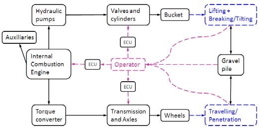
Wheel loader cost per ton per country [%]

                 100,0     3,5          3,8           3,2           1,7

                  90,0                                                         Fleet cost per ton

                  80,0                 30,4
                           45,1                      49,3                      Fuel cost per ton
                  70,0                                             58,8

                  60,0
                                                                               Operator cost per ton
                                       24,5
                  50,0
                                                      9,5
                  40,0     24,3                                     1,5        Repair and maintenance
                                       14,8                                    cost per ton
                  30,0                               16,0          17,0

                  20,0     11,7                                                Financial costs per ton
                                       26,6
                  10,0                               22,0          21,0
                           15,4
                   0,0
                         Europe
                         Germany   N. America
                                        USA     S. America
                                                    Brazil        Asia
                                                                   China

Figure 2, estimated fuel cost per ton for a wheel loader in a production chain, bucket applica-
tion. One country per region serves as an example and all other costs are crossed out due to
intellectual properties.
    This implies that fuel efficiency (ton/l) is an important aspect when purchasing a
wheel loader. However, not shown in this chart is that productivity (ton/h) is equally,
or more, important because if the production rate can’t be held then the whole produc-
tion site slows down, resulting in expensive loss of income.
The fuel efficiency and productivity of a production machine wheel loader in a bucket
application can be said to mainly depend on three major areas; the machine specifica-
tion, the working environment and the operator behaviour.
• The fuel efficiency and productivity due to the machine specification can be af-
    fected in three main ways;
    - Using the correct wheel loader size [2]. This is chosen by the customer, how-
        ever the dealer can help, using advanced software to simulate the customer site
        [3]. It is vital to have a machine big enough to be able to keep the productivity
        and to solve the specified work assignment. For instance a too small machine
        is not suitable for loading shot rock from face. It is however also important to
        not have a too big machine, if over-sized the fuel efficiency will decrease since
        the wheel loader will go on part load and not be fully utilized.
    - The equipment and attachment of the wheel loader; such as tyres and type of
        bucket. This is usually specified by the customer, but the dealer can help in the
        same way as in machine sizing, depending on the application and primary
        work assignment of the wheel loader [2,3].
    - The base machine efficiency, meaning the efficiency of the wheel loader itself,
        which is the sum of all the component of the wheel loader, everything from the
        engine to the transmission to the hydraulic system and, of course, also the
        complete machine control system. The machine efficiency is something the
        OEM are working really hard to increase [4,5] simply because it is a major
        competitive advantage to have a wheel loader with high fuel efficiency and
        productivity. This is due to the fact that uptime, productivity and fuel efficien-
        cy is some of the most important aspects when customers are choosing which
        machine they are going to purchase.
• The working environment, the site layout and the planning of the site is also im-
    portant to ensure maximum fuel efficiency and productivity. For example; not to
carry around material and stock-pile unnecessarily is a key to avoid loss in fuel
cost and productivity. The properties of the loaded material, such as excavation
severity and density, is also included here as an important parameter. The site
planning is mostly done by the customer but sometimes the dealer [3] or an exter-
nal company either give education [6] or helps planning the site.
• Last, but not least, [7] is the operator behaviour. This is the single most important
parameter after the machine is chosen and the site is planned. This means that dur-
ing the working life of a wheel loader the operator is the main parameter, together
with the assigned work task, that affects the fuel efficiency and productivity the
most. The traditional way to address the fuel efficiency and productivity differ-
ence due to operator behaviour distribution is operator training such as the Eco
Operator® training, or equivalent, [8,9] where a trainer coach the operator during a
number of days, providing tips and tricks to increase the fuel efficiency and, if
necessary, the productivity. A simpler alternative is to distribute manuals [10]
from where the operators can get some tips of operating the wheel loader in a
more efficient way.
2 Introduction
With the three major areas that affect the fuel efficiency and productivity; machine
specification, working environment and operator behaviour in mind then if analysing
a specific work assignment;
• The machine specification is, from a customer perspective, costly to affect once a
machine, with a certain equipment and attachment, is bought and chosen to do the
work assignment.
• Once the work site has been set up and made ready the working environment is
hard to affect since a chosen material is to be transported a decided distance ac-
cording to the specified work assignment.
• The operator behaviour however can be affected.
This means that the machine specification and the working environment is more in the
beginning when planning a site while the operator behaviour is a continuous occur-
rence. To cite a few voices within the construction industry;
"The biggest factors in fuel efficiency are properly trained operators and machine
maintenance," Chad Ellis, product and governmental sales manager, Doosan In-
fracore. [7]
"Both the machine design and operator play important roles in fuel economy," "Poor-
ly trained operators will cause even a good machine design to suffer poor fuel econ-
omy, and poor machine design will limit the fuel efficiency well-trained operators can
attain. Operators who ride the brakes on wheel loaders cause excessive fuel burn and
maintenance to the machine, for example." Jahmy Hindman, product marketing man-
ager for wheel loaders, Deere & Company. [7]
"The design of the loader is great, but all the design efforts are wasted if the operator
does not utilize the features. I feel the operator will play the most important role."
Nick Tullo, articulated haulers and wheel loaders, Volvo Construction Equipment. [7]
While it can be considered an established opinion that the operator plays a vital
part when considering fuel efficiency and productivity one might wonder why that is.
Well, focusing on a production machine wheel loader in a bucket application, it isimportant to understand the position of the operator in the control loop when a wheel
loader and its operator solve a specific work assignment.
To be able to explain the operator position in the control system a typical short
loading cycle, see Figure 3, is explained first.
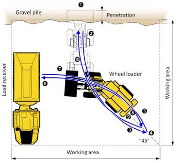
Figure 3, typical short loading cycle of a wheel loader onto a load receiver, also called Y-cycle
or V-cycle [12].
Assume that the wheel loader start at the reversing point, 4, driving forward towards
the pile and accelerating after just putting the machine into forward and decelerating
just before the pile. Then entering the pile, at 2, where the operator has to put pressure
on the front wheels to achieve friction enough to get the traction enough to penetrate
the pile. All this while lifting and tilting bucket while driving forward and completing
the bucket fill. After bucket fill is completed the operator put the machine into reverse
and accelerating backwards, decelerating just before the turning point 4. Then the
operator put the machine into forward, accelerating to later on decelerate again just
before the load receiver while during the complete traveling phase the operator has
lifted the bucket to ensure the precise height so that the emptying phase can begin. In
the emptying phase the operator is lifting and tilting to put the material in the correct
place onto the load receiver. Transporting and lowering the bucket towards the pile is
done in the same way as towards the load receiver but the other way around [12].
Supported by Figure 4, the control effort of the operator during the typical short
loading cycle in Figure 3 can be described as; when approaching the pile from the
revering point the operator has to not only transport the machine to the front of the
pile but also position the machine in a way that the machine goes into the pile at a
good entry point, both in regards to lateral and vertical position, depending on how
the pile looks like but also position the bucket in a way that the ground, i.e. worksite,
is not disturbed. Once in the bucket fill phase the operator has to start with enough
penetration to be able to lift enough material to ensure sufficient ground pressure to
guarantee enough traction to secure the capability to penetrate the gravel pile even
more to be able to fill the bucket while lifting and using the tilt to ensure to not get
stuck and tilt back the bucket at the correct time to minimize the time in the gravel
pile while at the same time maximizing the load in the bucket. The operator is all the
time during bucket fill balancing traction, which is non-linear due to the convertercharacteristics, and the working hydraulic that also depends on the speed of the en- gine. The tilt often also gets priority over the lift due to the lower pressure demand, resulting in that when using the tilt the lift speed get lower. To further complicate the steering has always priority, meaning that the speed of the lift and tilt depends on how fast the operator steer. The working hydraulics has also priority over the propulsion. This means that the accelerator pedal not only controlling the traveling but also some nonlinear traction and also the speed of the hydraulic pumps resulting in a dependence of the lift and tilt speed at a given position of the lift and tilt lever. The lift lever con- trols the lift speed of the bucket but also the longitudinal position of the bucket be- cause of the linkage layout. The tilt lever controls the angle speed of the bucket but also indirectly the lift speed due to the priority. And the only input the operator has is the viewing of the gravel pile and the speed of the different actuators, propulsion, lift and tilt, see Figure 4. Then while reversing from the gravel pile, changing to forward gear and then approaching the load receiver the operator has to ensure that the bucket have reached the correct height to be able to get over the edge of the load receiver and dump the material in the bucket. Everything under the same restrictions as during bucket fill, the lift speed is dependent on the engine speed that is controlled by the accelerator pedal that also control the machine speed. This results in a delicate choice of reversing point, 4, in Figure 3, depending on machine layout. When returning to the gravel pile the bucket has to be positioned once again [11]. Figure 4, schematic picture of the power balance and the control loop in a wheel loader during bucket fill [11,12]. ECU is a board computer. This line of argument results in, not totally surprising, that the operator is very much in the centre of the control loop, having a lot more input/outputs then driver of an on- road vehicle, e.g. a long-haul truck, see Figure 4. This, in turn, leads to that the opera- tor in a wheel loader, performing a specific work assignment, affect the fuel efficien- cy and productivity more than the on-road driver. In addition the performance indica- tors of a wheel loader operator is two dimensional, fuel efficiency (ton/l) and produc- tivity (ton/h), comparing to the driver that only have to concern about the fuel con- sumption (l/10km). An even more important aspect is that when an operator can’t hold a certain given production rate a lot more depend on this. A complete production chain can slow down if the wheel loader does not perform.
3 Method
With the main goal in mind, investigating the fuel efficiency and productivity differ-
ence of a wheel loader in a bucket application in a production chain caused by differ-
ences in operator behaviour, the most important was to try to eliminate all other pa-
rameters not affected by the operator but still have a as close to realistic condition as
possible. The decision was made to do the measurements in real world operations, not
in a simulator where it would be easier to control the machine and environmental
conditions. This was due to two main reasons; the simulator is just a model that does
not correspond to the real world, in respect to fuel consumption and loaded material in
the bucket, to the needed extent. Hence the fuel efficiency and productivity is hard to
get correct. The skill transfer is also not necessarily linearly from real world operation
to simulator [13], or vice versa, where some more inexperienced operator get a more
“video-game feeling”, not corresponding to how they would operate a wheel loader in
the reality, primarily with regards to risk-taking and safe operating.
    To avoid cycle-beating, and to investigate different degrees of difficulties when it
comes to bucket fill, three different bucket applications was investigated;
1. Short loading cycle onto a load receiver, see Figure 3, loading gravel. This would
    be a typical re-handling application where processed material has been stock-piled
    and then a wheel loader loads out-going trucks from the site from these stock-
    piles. See Figure 5.
2. Load and carry uphill to a pocket, loading gravel. This is a longer cycle than the
    short loading cycle in Figure 3 where the distance between point 4 and 6 is not
    10-15 m as in the short loading cycle but rather 100-150 m and the load receiver is
    exchanged to a hopper that goes to a conveyer belt. This would also be a typical
    re-handling application where pre-crushed material is stock-piled and then a wheel
    loader put this material into a hopper that goes to another crusher or sorting ma-
    chine, with settings depending on the customer demand. Another typical applica-
    tion this could correspond to is the stock-piling itself. See Figure 5.
3. Short loading cycle onto a load receiver, see Figure 3, loading rock. This would
    correspond to a face application where the wheel loader is loading blasted shot
    rock from face similar to Figure 1. This corresponds to the harder bucket fill ap-
    plication, meant to differentiate the operators a bit more than just loading gravel
    which is quite easy to fill the bucket with. See Figure 5.

Figure 5, the three different applications measured. From the right; short loading cycle gravel,
load and carry gravel and short loading cycle rock.

3.1 Measurements
As mentioned above, the most important was to isolate the operator behaviour as the
sole source of deviations. This was done by, in all three applications, using the same
machine with the same equipment and same bucket and same tyres in each application
for all operators to minimize the machine specification dependence and using the
same calibrated gravel pile to minimize the working environment dependence. The
same gravel was reused for all operators, in the hope that this would minimize the
deviation in bucket fill easiness, hence also differences in fuel efficiency and produc-
tivity, dependence due to material and environment deviation.
240 measurements á 20 min, 80 in each application, were done with 73 operators.
Four groups of operators was included in the study; 1) novice operators that has oper-
ated a wheel loader for 2-10 hours, 2) average operators that know how a wheel load-
er works but do not operate wheel loader as a profession, 3) internal professional
operators that are evaluating wheel loader and/or working as test operators and/or
show operators and/or trainers at Volvo, 4) external professional operators that are
working every day operating wheel loaders in bucket applications in production
chains as a profession.
The initial idea was to have 16 operators in each group, simply because this was
the highest reasonable number to measure in this large extent and still be able to
freeze the surrounding parameters machine specification and working environment.
However the measurements ended up with a few extra operators due to the fact that
when searching for external professional operators more than 16 customers showed
interest. And so it was decided by Volvo that all customers inquired should be al-
lowed to attend the event. Also some extra average was added because the personnel
that performed the measurements wanted to join the investigation.
Three of the most experienced internal test operators was asked to do so called in-
tensity measurements, meaning that they were supposed to operate the wheel loader in
three different intensities; 1) slow driving and low bucket fill factor, corresponding to
“Sunday driving”, 2) medium driving pace and medium bucket fill factor, correspond-
ing to what to expect when operating the wheel loader in 8 hour shifts, 3) as fast pos-
sible driving and as full bucket as possible, corresponding to a pace that only could be
held by an operator for less than one hour due to the high mental and physical work-
load on the operator. The reason for these intensity measurements was to map the
complete wheel loader working area in respect to productivity versus fuel efficiency.
All other operators was asked to operate the wheel loader in a pace corresponding to
how they would work in if they were supposed to do an eight hour shift with the spec-
ified work assignment.
Some factors was not possible to freeze during the complete measurement such as
the weather, so unfortunately the applications “load and carry uphill” and “short load-
ing cycle rock” that were made outside were affected by the weather conditions in a
way that the material is heavier when it is wet, hence it is easier to get higher produc-
tivity and fuel efficiency. The weather during the measurements were typical Swedish
late summer/early autumn which is very changing, meaning that the piles were pretty
moist all the measurement but in various level. In the “short loading cycle gravel” the
measurements were conducted inside so this measurement was unaffected by the
weather conditions.
During the measurements some more unexpected issues rose as well. The material
was worn a bit more than expected resulting in more fine material than expected re-
sulting in a higher density in the end of the measurements for the gravel applications,
especially the “load and carry” measurement. This results in that it was easier to get a
heavier load in the bucket in the end of the measurement, hence also easier to gethigher productivity and fuel efficiency. Also the wheel loader in the “short loading
cycle rock” had a minor problem with a hydraulic regulator, resulting in that for a
handful of operators that machine was a little harder to operate. There were also a
problem due to a faulty cable resulting in that the measurement system did not work
properly resulting in loss of data for a one external operator in the “load and carry
uphill” and five external operators in the “short loading cycle rock” resulting in an
odd number of operators.
Last, the rock application is not really representative to a real shot rock applica-
tion. This was done on purpose for two reasons; for once, if letting novice operator
operate in a shot rock application would be stupid due to safety risks due to risk of
slicing the tyres and second, the rock-like application that was used during the meas-
urement was more repeatable than shot rock could ever be arranged to be resulting in
that the pile can be seen as almost calibrated and same for all operators which
wouldn’t be possible using real blasted shot rock.
3.2 Analysis
As the main objective with this investigation was to identify the relation between
operator behaviour and fuel efficiency, and implicit also productivity, the main focus
when processing the data from the measurements was to measure the time and bucket
load as correct as possible because these parameters is the base for the fuel efficiency
and productivity calculations. The analysis was done in four levels;
The first level is on average for the complete run. On this level the most important
was to only count the wheel loader cycle. This means that when the articulated hauler
was away emptying in the “short loading cycles gravel or rock” or if there was any
problems with the conveyer belt in the “load and carry gravel” the fuel and time in the
wheel loader cycle should not be accounted for. This was done by instructing the
operators to stand still in neutral gear and then the data was recalculated so that the
dataset was shrunk to only include the time when the wheel loader was working. The
only source of fault in this level was that the weighing system sometimes misses a
load. The maximum allowed percentage of missed loads were set to twenty percent, if
the number of missed loads were higher than that the measurement was seen as cor-
rupt and not used. A correcting algorithm for this was constructed, adding an average
bucket load for every missed load. The confidence that the mean values are correct at
this level is very high.
The first level is used for evaluating operators comparing to each other in regards
to fuel efficiency and productivity. The reason why the evaluation is on average val-
ues is due to the fact that these are the values shown in the daily work.
The second level is on cycle basis. Here the fuel efficiency and productivity per
cycle is calculated. This is done by identifying a point in the working cycle that is
easy to detect and occur at the same time every cycle. Due to some problems with the
weighing system and unexpected operating behaviour, especially by the novice opera-
tors, the only point that were feasible to detect was the positioning point of the bucket
just before entering the pile. However this point can move a bit in the cycle depending
on whether or not the operator decides to scrape off and clean the ground on the way
into the pile. This results in that the cycle times is a bit more shaky, even though the
average is correct, the cycle time in the analysis can differ some seconds from the realvalue if using a stopwatch. This will affect the fuel efficiency and productivity for
isolated cycles.
The second level is used to see a pattern, regarding to 1st, 2nd and 3rd bucket onto
the load receiver and also for the operators to see what cycle is the best and how that
differ from the others, more or less learn from your own goods and bads. The cycle
values of fuel efficiency and productivity are also used to establish a trade-off curve
for that specific wheel loader in that specific work assignment. The trade-off curve
shows the highest possible fuel efficiency for a given productivity within the wheel
loader working area. Hence these trade-off curves can then be used to evaluate how
much better an operator can become in that application in that wheel loader. This
curve will of course depend on the number and skill level of the operators in the study
and is not an absolute truth but rather a way to show the method and how a tool could
look like if a larger base of operators could be reached. This is important to realize
when going from an empirical study like this to an estimation of fuel consumption
savings. This is a conservative way too look at the savings due to the fact that the
probability that the best operator in the world was in the study is small. Another im-
portant thing is that the highest fuel efficiency does not have to be the best for the
customer, if a higher productivity is demanded it is often fine to go down in fuel effi-
ciency. That is why it is important to get the trade-off curve for the complete working
area of the wheel loader and application in mind rather than just an optimal operating
point. Reasoning in the same way, it is only possible to increase productivity, allow-
ing higher fuel efficiency if the site conditions allow intermittent operation.
The third level is on phase [14,15,11,12] basis. Here the cycles are divided into
three phases; “Bucket Fill”, “Bucket Empty” and “Transport”. These phases are dis-
tinguished by a number of conditions resulting in that the “Bucket Fill” is everything
from when the bucket get close enough to the ground until the operator set the gear
shift lever in reverse and leaving the pile, “Bucket Empty” is more or less from when
the operator rises the bucket to a certain height and then until the bucket comes down
to a lower height again after moving towards the load receiver and then emptying and
then started to reverse from the load receiver. “Transport” is the rest, loaded and un-
loaded, forward and reverse. The difficulties in the second level applies in this level
too, resulting in that the exact time for the phase division is not achieved but rather an
approximate point in time.
The third level is used to see what did go right or wrong in closer detail than on
complete cycle level and also how each phase correlate to each other and to the com-
plete cycle performance value. From this it can be concluded which phase is the most
important for a specific operator to adjust to increase the fuel efficiency and produc-
tivity and what in the phase that has to be adjusted.
The forth level is not actually another level but rather a way to break down and
show the operator what happened during a specific cycle, or phase, showing individu-
al signals. Here individual signals show what the operator feels, hears or sees, for
example engine torque, engine speed or actuator (lift, tilt, propulsion) speed on one
hand and then the signals the levers and pedals the operator uses, such as lift, tilt lever
and accelerator and brake pedal. In that way the operator can recognize the system,
and really analyse the operator behaviour, when getting the feedback from the pro-
posed training tool, see chapter 4.2. It is also on this level each operator can compare
with the “Shadow operator” which is the “optimal” operator. In this study that is thebest operator in the study but it could also be a virtual operator calculated by a com-
puter, especially if the training is done in a simulator environment.
After investigating and comparing between the three different applications the
conclusion was that the weather, worn of material and hydraulic controller malfunc-
tion addressed in chapter 3.1 was not affecting the analysis to any larger extent hence
the results are valid but one can still have these factors in mind.
4 Results
All the results is based on that the fuel efficiency and productivity are most important.
The machine specification and the working environment are considered to be fixed for
each and one of the three applications investigated. Hence things like operability and
work assignment are implicitly also fixed.
4.1 Fuel efficiency and productivity distribution due to operator behaviour
The main result in regards to fuel efficiency and productivity is that the difference
between different operators is huge! One operator can have five to eight times higher
productivity than another, depending on application, whiles the difference between
two other operators can be two to three times higher fuel efficiency for one comparing
to the other, see Figure 6.
SLC gravel LAC gravel
35 14
EP EP
IP IP
30 12
IA IA
IR IR
25 10
20 8
ton/l
ton/l
15 6
10 4
5 2
0 0
0 200 400 600 800 1000 1200 0 50 100 150 200 250 300 350 400 450 500
ton/h ton/h
SLC rock
25
EP
IP
IA
20
IR
15
ton/l
10
5
0
0 100 200 300 400 500 600 700 800 900
ton/h
Figure 6, the fuel efficiency and productivity for the different operators. EP is the external
professional, IP is the internal professional, IA is the average and IR is the novice operators.
SLC is short loading cycle and LAC is load and carry. (Note that the ticks is not the same in the
different applications)It is however a bit unfair to compare the extremes since an operator is not that
novice for a long period of time. However even if the novice operators are excluded
the productivity is two to four times higher and the fuel efficiency is 1.5 to 2.5 times
higher, as can be seen in Figure 6. The exception is of course day-to-day workers,
many with no experience, but this is rather unusual looking at the world market.
Another interesting thing is that both the fuel efficiency and the productivity
seems to have a more or less linear dependence regards to the experience, or skill
level, of the operators, meaning that a y=kx+m line could be drawn in Figure 6. The
closer an operator is to the up right corner, the more experienced operator. One excep-
tion is however some of the intensity measurements where the test operators were
asked to stress the machine to an abnormal behaviour.
Another interesting result that can be seen in Figure 6 is the dependence on appli-
cation, in the short loading cycle gravel the operator is somewhat closer to each other
than in the other applications. In the load and carry gravel this is resulting from that
the bucket fill factor is much more important in this application due to the fact that the
load are going to be transported such a distance using a larger amount of fuel in the
“Transport” phase only a small difference in the bucket fill factor results in large
differences in fuel efficiency and productivity. In the rock application the larger dif-
ference is mostly because it is much more difficult to fill the bucket with the material
in the rock application but also what kind of material that ends up in the bucket, large
rocks or a lot of fine material, resulting in a much larger deviation between the opera-
tors and individual cycles.
As mentioned in chapter 3.2 each cycle fuel efficiency and productivity was also
calculated. Interesting here is that every operator in itself has a quite large deviation
from the mean fuel efficiency/productivity. In Figure 7 the cycle distribution of oper-
ator IA1 is shown, with the average value marked with a larger marker, together with
all the other operator average. The results from this implies that if operator IA1 oper-
ate the wheel loader at the best point achieved then the mean fuel efficiency would
increase with about 10-15 percent and the productivity by roughly 10 percent. Alter-
natively the operator could increase the productivity by about 20 percent and the fuel
efficiency by a few percent, all depending on the current site boundary conditions.
SLC gravel
35
IA1
Other
30
25
20
ton/l
15
10
5
0
0 200 400 600 800 1000 1200
ton/h
Figure 7, the fuel efficiency and productivity distribution of one operators cycles comparing to
the other operators average. The larger IA1 marker corresponds to the mean IA1 cycle and the
smaller are each individual IA1 cycles.To be completely fair the assumption is not 100% correct since some deviation be-
tween the buckets when loading a load receiver is inevitable since the 3rd bucket onto
the load receiver has to be positioned more carefully to not spill material off the load
receiver. However similar behaviour is apparent in all three applications, short load-
ing cycle in gravel is shown as an example in Figure 7.
To get the trade-off curve, mentioned in chapter 3.2, two approaches can be con-
sidered. Either the convex hull of all the operators average cycles in Figure 6 that will
represent a Pareto front that is called the trade-off curve or each and one of operators
individual cycles, as IA1’s example in Figure 7, is plotted in the same plot and the
convex hull from this is taken as the trade-off curve. However due to the concerns
regarding the cycle time raised in chapter 3.2 the convex hull has to be slightly modi-
fied to take away unreasonable points. This could however be avoided with better
measurement equipment. In Figure 8 the two different trade-off curves are plotted
using the two different methods mentioned above.
SLC gravel
50
Mean
45 Max
EP
40
IP
IA
35
IR
30
ton/l
25
20
15
10
5
0
0 200 400 600 800 1000 1200 1400
ton/h
Figure 8, all the operator’s individual cycles with the trade-off curves from the average,
“Mean”, cycles and from the individual cycles, “Max”.
The reasoning is that the “Max” trade-off curve, which is the modified convex hull
for all the individual cycles, is the real trade-off curve for this specific wheel loader in
this specific work assignment. Short loading cycle in gravel is shown as an example
in Figure 8 but similar can be seen in the other two applications.
These both approaches are under the assumption that the measurements has been
done on infinite number of operators. Considering that this is not the case, the method
still work and the only difference is that the estimations can be seen as a bit on the
conservative side due to the fact that the probability that all the best operators in
world attended this study is very small.
However important to mention here is that the fuel saving between these two
curves that one might think is realistic for all the operators in this study is not really a
reality since there are some difference between 1st, 2nd and 3rd bucket when loading
onto a load receiver due to the positioning of the load when unloading the 3rd bucket.
This has to be accounted for. But for the “fleet” of operators in this study the “Mean”
curve should be able to be raised to around half of the distance between the two
curves, meaning around 10 percent fuel efficiency increase, depending on the produc-
tivity demand. If the conditions on the site allow part engine-off time then a lot morecould be saved of course, then only operating the wheel loader at the optimal produc-
tivity resulting in up to around 20 percent fuel efficiency increase. This also means
that if the site manager knows the trade-off curve for the specific application and the
specific wheel loader on the site, then the site can be planned after that, optimizing the
complete site fuel efficiency.
The reason why the trade-off curve looks like it does can be explained by just set-
ting up the equations for the different system in a wheel loader. The reason why both
fuel efficiency and productivity goes towards zero is not that surprising. If just stand-
ing still, or just driving around then fuel and time will be wasted and no material
moved, hence zero productivity and zero fuel efficiency. The reason why the trade-off
curve then flattens and finally goes down a bit is due to the fact that there are compo-
nents with speed related losses that increase in square and also components that is
trimmed to have their maximum efficiency at lower speeds than the ones that are
necessary when the wheel loader is stressed to its maximum capacity.
Fuel efficiency and productivity for each phase was also calculated but was decid-
ed not to be shown here simply because these parameters was no good indicator of
how well each phase were performed. The conclusion was that an operator can cheat
in one phase, for example in the bucket fill, by only filling the bucket very little and
very quick, by using only the machine inertia. In that case an operator can get very
high fuel efficiency and productivity in the bucket filling phase, but losing a lot in the
other two phases, transport and bucket empty. This due to that there are very little
load in the bucket resulting in very low fuel efficiency and productivity in the com-
plete cycle due to the much lower payload percentage. However, as indicated in the
text above there was a clear connection of a well performed bucket fill phase, mean-
ing a lot of load in the bucket to a low amount of fuel, and a well performed cycle,
meaning high fuel efficiency and productivity. This indicates that the “Bucket Fill”
phase is important for the complete cycle performance.
4.2 Training tool
The proposed training tool works just as well in a simulator as in a real wheel loader
and there are of course benefits and drawbacks with both of them. In the real wheel
loader the difficulties to measure, to have a calibrated gravel pile and to take the
weather into account, the travelling for the operators and so on have already been
touched upon in previous chapters. In the simulator the problem is more of the “play-
ing a video-game feeling” [13] and that it is still not the same as a real wheel loader
has already been touched upon in previous chapter and there are also barriers for
using simulators in operator training of construction equipment [16].
The proposed training tool is built in a way that; the tool chooses what is consid-
ered the optimal operator given the circumstances. This means that for a given base of
operators the tool chooses the one that has the highest fuel efficiency, if that is the
criteria, the criteria can for example just as well be productivity. In the example in this
paper the optimal operator is chosen to the one with the highest average fuel efficien-
cy but the optimal operator could just as well be chosen to be the operator with the
cycle with the highest fuel efficiency. Or it could be a virtually composed operator
from three different operators, each and one best in the three phases, bucket fill,
transport and bucket empty. In a future edition the optimal operator can be a computer
computed operator, especially in a simulator edition.The training tool takes this optimal operator and set this to be the “Shadow opera-
tor” and this is what the operator compares themselves to. The idea is that the opera-
tors that joined the training should be able to understand what the “optimal” operator
did that the operator did not do. For that sake the training tool is built up in the three
levels discussed in chapter 3.2. The idea is that the operator identifies where the oper-
ator is, in regards to fuel efficiency and productivity, compared to the “Shadow opera-
tor”. This is done in a plot like the one in Figure 6. Once that has been done the oper-
ators own potential in analysed in a plot like Figure 7 coming to the conclusion that if
the operator should have operated the wheel loader as efficient as at the best cycle
how close would the operator be comparing to the “optimal operator” be then? Then
the operator goes one level deeper and start to look at individual parameters, such as
cycle time and load in the bucket, in individual cycles that has a direct correlation
with the fuel efficiency and productivity, this can look like Figure 9. The operator
also gets the fuel efficiency and productivity in histogram shape so that the correlation
between a well performed cycle and how the operator controlled the wheel loader in
that particular cycle can be done.
SLC gravel SLC gravel
45 9000
40 8000
35 7000
30 Load weight [kg] 6000
Cycle time [s]
25 5000
20 4000
15 3000
10 Shadow Operator Cycle time 2000 Shadow Operator Load
IA1 Cycle time IA1 Load
5 Shadow Operator adv Cycle time 1000 Shadow Operator adv Load
IA1 adv Cycle time IA1 adv Load
0 0
0 2 4 6 8 10 12 14 16 18 0 2 4 6 8 10 12 14 16 18
Cycle number [-] Cycle number [-]
Figure 9, the cycle time and load in the bucket per cycle is shown as example histogram from
the training tool highest level.
Already at this level, reasons can be seen why the operator A1 gets lower fuel ef-
ficiency and productivity than the “Shadow operator”. This is because the cycle times
are too long and the bucket loads is too low, both resulting in lower fuel efficiency
and productivity.
To understand why these high level parameters, for example the cycle time and
bucket load, ended up as they did the operator can go one level deeper and analyse all
the parameters in Table 1 and how the operator’s histograms differ from the “Shadow
operator”. The idea here is that the operator should be able to imagine how it was in
the wheel loader when operating, so all the impressions from the wheel loader should
be represented in the histograms, everything from hearing and feeling the speed and
torque of the engine to seeing the velocity of the machine and on the lift and tilt to
how the operator actually actuates the three different actuators; propulsion, lifting and
tilting. An example of how this level can look like is shown in Figure 10.SLC gravel SLC gravel
160 140
Shadow Operator Shadow Operator
140 IA1 IA1
120
Shadow Operator adv Shadow Operator adv
IA1 adv IA1 adv
120
100
100
80
Time [s]
Time [s]
80
60
60
40
40
20 20
0 0
700 800 900 100011001200130014001500160017001800190020002100 0 1 2 3 4 5 6 7 8 9 10 11
ICE Speed [rpm] Vehicle speed [km/h]
Figure 10, examples of histogram from the training tool mid-level showing how much time per
cycle in average the operator has spent in each engine speed and machine velocity bin.
At this level the operator A1 can start to get the understanding of why the cycle
time is higher than for the “Shadow operator”. The operator A1 has much more stand-
ing still time per cycle, in this case in the “Bucket Empty”, also the speed of the ma-
chine is lower indicating that the transport phase takes longer time, both visible in the
next, lower level. It also shows is that the operator A1 does not utilize the engine as
much as the “Shadow operator”, to know how this affect the load the “Bucket Fill”
can be analysed at the next level where the cycles has been broken up in the three
phases “Bucket Fill”, “Transport” and “Bucket Empty”, an example of how that can
look like, when looking on how the actuators are controlled is visible in Figure 11.
SLC gravel
20
Shadow Operator
18 IA1
Shadow Operator adv
16 IA1 adv
14
12
Time [s]
10
8
6
4
2
0
0 10 20 30 40 50 60 70 80 90 100
Accelerator pedal position @ BucketFill [%]
SLC gravel SLC gravel
80 100
Shadow Operator Shadow Operator
IA1 90 IA1
70
Shadow Operator adv up Shadow Operator adv up
Shadow Operator adv down 80 Shadow Operator adv down
60
IA1 adv up IA1 adv up
70
IA1 adv down IA1 adv down
50
60
Time [s]
Time [s]
40 50
40
30
30
20
20
10
10
0 0
-125 -100 -75 -50 -25 0 25 50 75 100 125 -125 -100 -75 -50 -25 0 25 50 75 100 125
Lift lever @ BucketFill [%] Tilt lever @ BucketFill [%]
Figure 11, examples of histogram from the training tool lowest level showing how much time
in the bucket filling phase in average the operator has spent in each actuator controller bin.And once again it is visible for the operator A1 what could be improved the next
time, in this case it is simply, for all actuators that the operator A1 is too gentle and
cannot control the wheel loader as fast as the “Shadow operator”. This means that to
get the same fuel efficiency and productivity as the “Shadow operator” the operator
IA1 has to utilize more of the wheel loader capacity to a larger extent. To be able to
do that the IA1 operator has to learn how to control the wheel loader faster.
In this paper all the axes has been crossed out due to intellectual properties. How-
ever in the real training tool this will of course be visible. The method is however the
same.
Table 1, Content of the training tool in regards to the different levels mentioned in chapter 3.2.
Parameter Unit Average Per cycle Per phase
Fuel efficiency [ton/l]
Productivity [ton/h]
Load weight [kg]
Cycle time [s]
Phase time [s]
Accumulated fuel [l]
Fuel consumption [l/h]
Distance [m]
Speed [km/h]
Accelerator pedal position [%]
Load sensing pressure [MPa]
Engine torque [Nm]
Brake pressure [kPa]
Brake pressure @>0.5km/h [kPa]
Engine speed [rpm]
Engine power [kW]
Gear [-]
Lift angle speed [mRad/s]
Tilt angle speed [mRad/s]
Lift lever [%]
Tilt lever [%]
Lift angle [mRad]
Tilt angle [mRad]
Lift angle @ F→R [mRad]
5 Conclusion
The most important conclusion that can be drawn from this study is the vital part
for fuel efficiency and productivity the operator plays. Fuel efficiency increases of up
to three times, or 200%, and productivity increases of up to eight times, or 700%,
between novice and professional operators can be seen and if the novice operators are
excluded fuel efficiency increases of up to two and a half times, or 150%, and produc-
tivity increases of up to four times, or 300% is visible. This means really big poten-
tials in cost savings! This means that this should be a key area for continued research
within the construction industry.
An interesting conclusion is as well that the fuel efficiency and productivity level
seems to be linear to the experience, or skill level, resulting in that a site manager can
quite easy calculate the payback time of a training fee.Interesting is also that the application seems to play an important role, meaning
that even if a site manager employ an experienced operator it could be useful to train
the operator on that specific application if that differ a lot from what the operator is
used to.
Interesting is also the deviation from the average for a single operator in one spe-
cific application. That one operator could deviate from the mean by ±10-20 percent
both regarding fuel efficiency and productivity shows the potential in letting the oper-
ator know the importance of these things and maybe even have a bonus system, en-
couraging the operators to do their best in regards to fuel efficiency and productivity
as well as solving the work assignment.
An interesting result regarding the trade-off curves is that, if a site manager knows
the trade-off curves, the manager can control the choice of wheel loader size, set the
pace of the production and optimize the overall efficiency of the complete site. This
requires of course that the trade-off curves for all the machinery in the site is known
and a total site optimization is done based on all the trade-off curves.
The main conclusion regarding the training tool is that it is possible to just record
a number of operators and then let a computer do an automated analysis and then
present the results to the operators in different levels. Then the operator can analyse
the behaviour and realize what to do better the next time. And due to the fact that not
even the best operator will reach the “max” curve in Figure 8, with the mean cycle
values all operators have something to learn in this training tool. The really nice thing
with this training tool is that until the virtual, or computer calculated “optimal” opera-
tor is done in a robust way it can just as well be used with only real operators, in sim-
ulator or real world. Especially if a really good specialist trainer comes along and
operate the wheel loader in the same pile.
The training tool is, of course, most powerful in the hands of a competent trainer
who can interpret the results in a way so that the operator understands the feedback
the best.
All the conclusions, and many of the algorithms, can be applied to developing of
an advanced operator assist system [17].
6 References
1. Hendley, N. (March 2011) Take a load off in On-Site.
2. Energy Best Practice Guide for Tractors – Fleet/Site Managers, Skanska,
http://www.skanska.com/global/About%20Skanska/Sustainability/Responsibility/33Tractor
Man%20010508.pdf
3. http://sitesim.net/
4. Doosan DL300 wheel loader offers productive, fuel-efficient operation,
http://www.doosanequipment.com/dice/news/pressreleases/pr-dl300.page
5. Volvo Construction Equipment OPTIshift,
http://www.volvoce.com/SiteCollectionDocuments/VCE/Documents%20Global/wheel%20
loaders/LaunchBrochure_Optishift_L150F-L180F-L220F_EN_20021064-A.pdf
6. Performance Optimization Training,
http://www.quarryengineers.com/Performance_Optimization_Training.html
7. Bennink, C. (April 2009) Wheel Loader Designs Squeeze Out More Fuel Efficiency With-
out Sacrificing Productivity - Squeeze Fuel Costs in forconstructionpros.com.8. http://www.volvoce.com/constructionequipment/europe/en-
gb/products/eco_operators/Pages/Volvo_Eco_driving.aspx
9. http://www.minemachinetraining.com.au/wheel-loader-training-course.html
10. Loader Operator TRAINING MANUAL (Sample Pages) 992 G Wheel Loader,
http://www.north-pacific.ca/LoaderManual-Sample-English.pdf
11. Filla, R. (2011) Quantifying Operability of Working Machines, ISBN 978-91-7393-087-1
12. Filla, R. (2005) Operator and Machine Models for Dynamic Simulation of Construction
Machinery, ISBN 91-85457-14-0.
13 Phillip S. Dunston, Robert W. Proctor & Xiangyu Wang (2011) Challenges in evaluating
skill transfer from construction equipment simulators, Theoretical Issues in Ergonomics
Science, DOI:10.1080/1463922X.2011.624647.
14 Bohman, M. (2005) On Predicting Fuel Consumption and Productivity of Wheel Loaders,
ISSN: 1402-1617.
15 Karlsson, J. (2010) Analyzes of a wheel loader usage.
16 Fjeldheim Ek, D., Mulisic, A., Syta, F. (2010) Entry barriers on the training simulator
market for construction vehicles in Europe.
17 Frank, B (2012) On Reducing Fuel Consumption by Operator Assistant Systems in a Wheel
Loader, submitted to Advanced Vehicle Technologies and Integration.
(Internet links verified 2011-12-12)You can also read


