The Lottery Ticket Hypothesis: Finding Small, Trainable Neural Networks
←
→
Page content transcription
If your browser does not render page correctly, please read the page content below
The Lottery Ticket Hypothesis: Finding Small,
                                                         Trainable Neural Networks

                                                            Jonathan Frankle                             Michael Carbin
                                                               MIT CSAIL                                   MIT CSAIL
                                                        jfrankle@csail.mit.edu                       mcarbin@csail.mit.edu
arXiv:1803.03635v3 [cs.LG] 20 May 2018

                                                                                       Abstract
                                                  Neural network compression techniques are able to reduce the parameter counts of
                                                  trained networks by over 90%—decreasing storage requirements and improving
                                                  inference performance—without compromising accuracy. However, contemporary
                                                  experience is that it is difficult to train small architectures from scratch, which
                                                  would similarly improve training performance.
                                                  We articulate a new conjecture to explain why it is easier to train large networks:
                                                  the lottery ticket hypothesis. It states that large networks that train successfully
                                                  contain subnetworks that—when trained in isolation—converge in a comparable
                                                  number of iterations to comparable accuracy. These subnetworks, which we term
                                                  winning tickets, have won the initialization lottery: their connections have initial
                                                  weights that make training particularly effective.
                                                  We find that a standard technique for pruning unnecessary network weights natu-
                                                  rally uncovers a subnetwork which, at the start of training, comprised a winning
                                                  ticket. We present an algorithm to identify winning tickets and a series of exper-
                                                  iments that support the lottery ticket hypothesis. We consistently find winning
                                                  tickets that are less than 20% of the size of several fully-connected, convolutional,
                                                  and residual architectures for MNIST and CIFAR10. Furthermore, winning tickets
                                                  at moderate levels of pruning (20-50% of the original network size) converge up to
                                                  6.7x faster than the original network and exhibit higher test accuracy.

                                         1   Introduction
                                         Neural networks tend to be dramatically over-parameterized [51]. Techniques for eliminating
                                         unnecessary weights (pruning) [31, 18, 17, 38, 34] and training small networks to mimic large ones
                                         (distillation) [2, 21]) demonstrate that the number of parameters can be reduced by more than 90%
                                         while maintaining accuracy. Doing so diminishes the size [17, 21] or energy consumption [50, 33, 39,
                                         36] of trained networks, making inference more efficient. If a network can be so compressed, then the
                                         function it learned can be represented by a far smaller network than that used during training. Why,
                                         then, do we train large networks when we could improve efficiency by training smaller networks
                                         instead? In practice, large networks are easier to train from the start than small ones [17, 5, 21, 51].
                                         In this paper, we add to the body of evidence and theory about why large networks are easier to train
                                         by articulating the lottery ticket hypothesis. It states that any large network that trains successfully
                                         contains a subnetwork that is initialized such that—when trained in isolation—it can match the
                                         accuracy of the original network in at most the same number of training iterations.
                                         We designate these subnetworks winning tickets since they have won the initialization lottery with
                                         a combination of weights and connections capable of training. We find that a standard pruning
                                         technique [17] automatically uncovers winning tickets. When randomly reinitialized, the winning
                                         tickets that we discover no longer match the performance of the original network, suggesting the
                                         importance of the original initialization.

                                         Preprint. Work in progress.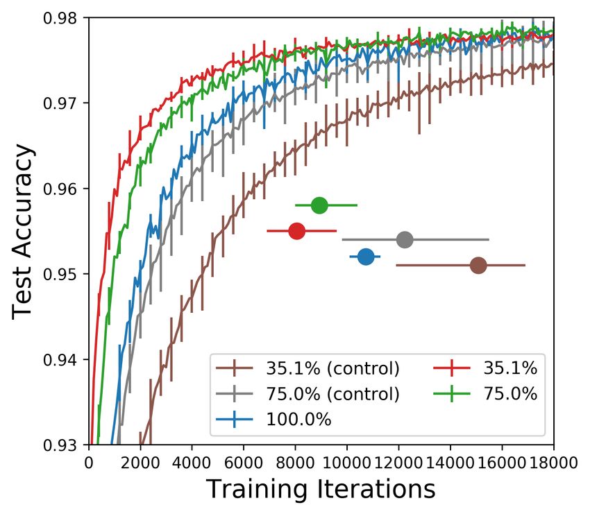
Returning to our motivating question, we extend the lottery ticket hypothesis into the conjecture (that
we do not empirically test) that large networks are easier to train because, when randomly initialized,
they have more combinations of subnetworks from which training can recover a winning ticket.

Methodology. To evaluate the lottery ticket hypothesis experimentally, we identify winning tickets
in large networks by training and subsequently pruning the smallest-magnitude weights [17]. The
set of connections that survives this pruning process is the architecture of a winning ticket. Unique
to our work, the winning ticket’s weights are the values to which these connections were initialized
before training began. This forms our central experiment:

      1. Randomly initialize a neural network.
      2. Train the network until it converges.
      3. Prune a fraction of the network.
      4. To extract the winning ticket, reset the weights of the remaining portion of the network to
         their values from (1)—the initializations they received before training began.

If large networks contain winning tickets and pruning reveals them, then the lottery ticket hypothesis
predicts that the pruned network—when reset to the original initializations—will maintain competitive
accuracy and convergence times at sizes too small for a randomly-initialized or a randomly-configured
network to do the same.

Research questions and results. In this paper, we investigate the following questions:
How does the lottery ticket hypothesis manifest for different networks? We identify winning tick-
ets in a fully-connected architecture for MNIST and convolutional and residual architectures for
CIFAR10 [29], including networks with dropout [48], Xavier initialization [12], and batch normaliza-
tion [26]. On a resnet trained with momentum, we could not find a winning ticket.
How large are winning tickets? When we find winning tickets, they are 20% (or less) of the size of
the original network and match its convergence times and accuracy.
How effectively do winning tickets train compared to the original network? Winning tickets pruned by
50% to 70% converge in 1.2x-6.7x fewer iterations while surpassing the original network’s accuracy.
What is the structure and initialization of a winning ticket? When randomly reinitialized or rear-
ranged, winning tickets perform far worse than the original network, meaning neither structure nor
initialization alone is responsible for a winning ticket’s success. Fully-connected winning ticket
initializations are the extremes of the truncated normal distribution from which they were sampled.

Contributions.

      • We propose the lottery ticket hypothesis as a new perspective on neural network training.
      • We demonstrate that pruning uncovers the winning tickets predicted by the lottery ticket
        hypothesis, making it possible to extract small, trainable networks from larger networks.
      • We apply this technique to empirically evaluate the lottery ticket hypothesis on fully-
        connected, convolutional, and residual networks. The evidence we find supports both the
        lottery ticket hypothesis and our contention that pruning can extract winning tickets.
      • We show that winning tickets at moderate levels of pruning converge in fewer iterations and
        reach higher accuracy than the original network.

Implications. In this paper, we mainly measure the lottery ticket hypothesis, which requires
repeatedly training and pruning a network. Now that we have demonstrated the existence of winning
tickets, we hope to design training schemes that exploit this knowledge. Since winning tickets can
be trained from the start in isolation, it would be beneficial to identify them as early as possible
in the training process or to integrate lessons from winning tickets directly into the design of new
architectures and initialization schemes. Techniques that prune networks during training [35, 38, 41]
might already identify winning tickets and could benefit from making this an explicit goal.

                                                  2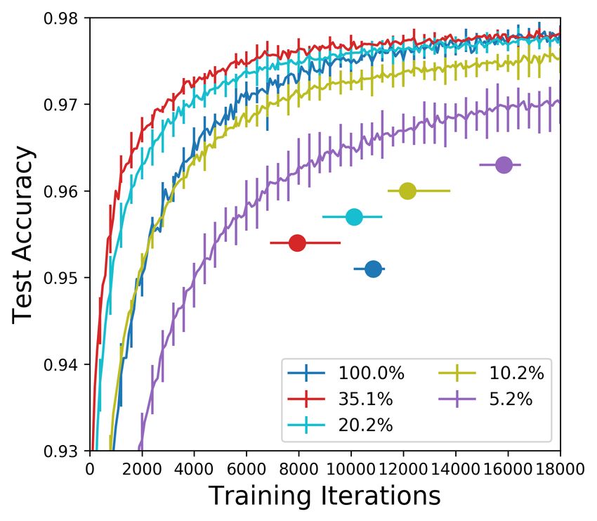
Network lenet [30] conv2 [30] conv4 [43, 6] resnet18 [19]
3x3x64, 3x3x64 3x3x16, 3x[3x3x16, 3x3x16]
5x5x64, pool pool, 3x3x128 3x[3x3x32, 3x3x32]
Convolutions 5x5x64, pool 3x3x128, pool 3x[3x3x64, 3x3x64]
FC Layers 300, 100, 10 384, 192, 10 256, 256, 10 avg-pool, 10
All/Conv Weights 266K 1.75M / 107K 1.15M / 260K 271K / 270K
Init. / Epochs N (0, 0.1) / 50 N (0, 0.1) / 30 Normal Xavier / 20 Normal Xavier / 85
Optimizer SGD(0.05) SGD(0.01) SGD(0.003) SGD(0.1, 0.01, 0.001)
Figure 1: Architectures tested in Sections 2, 3, 4, and 5. Square brackets are residual layers. Normal
distributions are truncated at two standard deviations from the mean.
2 Winning Tickets in Fully-Connected Networks
In this section, we assess the lottery ticket hypothesis as applied to fully-connected networks trained
on MNIST. We use the lenet-300-100 architecture [30] as described in Figure 1. We follow the outline
from Section 1: after randomly initializing and training a network, we prune the network and reset
the remaining connections to their original initializations. We use a simple pruning heuristic: remove
a percentage of the weights with the lowest magnitudes within each layer (as in [17]). Connections to
outputs are pruned at half of the rate of the rest of the network to avoid severing connectivity.
We test two pruning strategies: one-shot pruning and iterative pruning. One-shot pruning prunes
all at once in a single step after training. Iterative pruning repeatedly trains, prunes, and resets the
weights, removing more of the network on each iteration of the process.
2.1 Results
One-shot pruning. Winning tickets found via one-shot pruning converge faster than the original
network. Figure 2 plots the test set accuracy and convergence behavior during training of winning
tickets pruned to different levels.1 Each curve is the average of five runs starting from randomly
initialized networks; error bars are the minimum and maximum of any run. A dot with error bars
shows the average, minimum, and maximum convergence time for the curve in the same color.
For the first few pruning steps, convergence times decrease and accuracy increases (left graph in
Figure 2). A winning ticket comprising 90% of the weights from the original network converges
faster than the original network but slower than when pruned to 75%. This pattern continues until
1
We define convergence as the moment at which the 1000-iteration moving average of test loss changed by
less than 0.001 for 1000 consecutive iterations. We measured test accuracy every 100 iterations. Measuring
convergence is an imprecise art, but this metric seems to adequately characterize the behavior for our purposes.
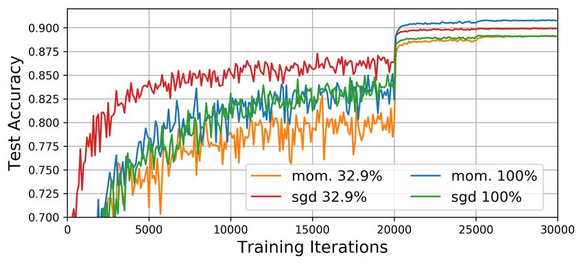
Figure 2: Test accuracy on the fully-connected network (one-shot pruning) as training proceeds.
Each curve is the average of five trials. Percents are the fraction of weights remaining in each layer
after pruning. Error bars are the minimum and maximum of any trial. Dots are the time when the
corresponding colored curve converges; error bars are the earliest and latest convergence times.
3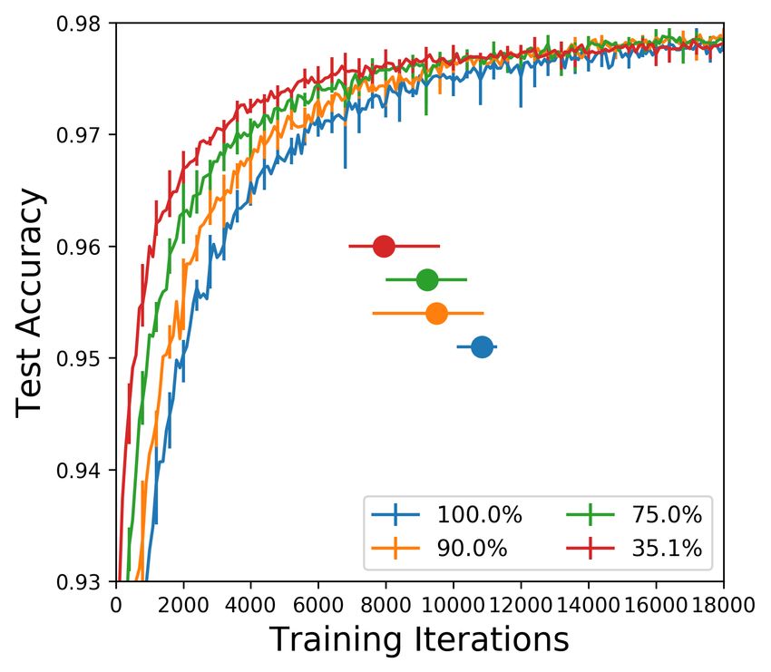
Figure 3: Convergence behavior and accuracy of the fully-connected network under one-shot (top)
and iterative (bottom) pruning. Error bars are the minimum and maximum value any trial took on.

55%, after which convergence times flatten and, after 35%, increase (middle graph). When pruned to
between 10% and 15%, a winning ticket regresses to the performance of the original network.
The top of Figure 3 summarizes this behavior for all pruning levels. On the left are convergence times
in relation to pruning level; on the right is accuracy at convergence. When pruned to between 70%
and 35%, the average winning tickets converge at least 22% faster and are more accurate than the
original network. Further pruning causes convergence times and accuracy to degrade.

Iterative pruning. Figure 3 (bottom) shows the results of iteratively pruning by 20% per iteration
(red). One-shot data from Figure 3 (top) is reproduced in blue. Iteratively-pruned winning tickets
converge faster and reach higher accuracy at smaller network sizes than one-shot pruned networks.
Convergence times flatten when pruned down to between 41% (38% faster than the original network)
and 21% (33% faster). The average winning ticket returns to the original convergence time when
pruned to 2.9% and the original accuracy when pruned to 3.6%.
Although iterative pruning extracts smaller winning tickets, repeated training means they are costlier
to find. However, we aim to analyze the behavior of winning tickets rather than to find them efficiently.
Iterative pruning’s advantage is that it puts a tighter upper-bound on the size of a winning ticket.

2.2   Control Experiments

The lottery ticket hypothesis predicts that winning tickets train effectively due to a combination
of initialization and structure. To compare the importance of these factors, we ran two control
experiments: (1) retain structure but randomize initializations and (2) retain initalizations but randomly
rearrange structure. We trained three controls for each winning ticket (15 in total). We find that
structure seems more important, but neither factor alone explains the efficacy of a winning ticket.

Random reinitialization. This experiment evaluates the importance of the winning ticket’s initial-
ization by reusing its structure but randomly reinitializing its weights from the original distribution.
The right graph in Figure 2 shows this experiment for one-shot pruning. In addition to the original
network and winning tickets at 75% and 35%, it has two curves for the controls. The broader results
of this experiment are the orange lines in Figure 3. Unlike winning tickets, the controls converge
increasingly slower than the original network and lose accuracy after little pruning. The average
iterative control’s accuracy drops off from the original accuracy when the network is pruned to about
51%, compared to 3.6% for the winning ticket. This experiment supports the lottery ticket hypothesis’
emphasis on initialization: the original initialization withstood and benefited from pruning, while the
random reinitialization’s performance immediately suffered and diminished steadily.

Random rearrangement. This experiment evaluates the importance of structure by randomizing
the locations of a winning ticket’s connections within each layer while retaining the original initial-
izations (green lines in Figure 3). The rearranged networks perform slightly worse than the previous
experiment—convergence times increase even faster and accuracy drops off earlier—suggesting that

                                                    4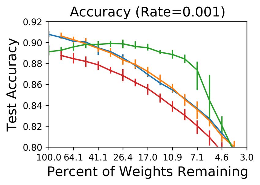
Figure 4: Convergence times and accuracy for Questions 1 and 2 (pruning and random reinitialization).

                (a) Conv2 architecture                                (b) Conv4 architecture
Figure 5: Convergence times and accuracy for Question 3 (pruning convolutions vs. fully-connected).

structure is more important than initialization. However, in general, the control experiments indicate
that winning tickets emerge from a combination of initialization and structure; neither initialization
nor structure alone explained the better performance of winning tickets.

3       Winning Tickets in Convolutional Networks
In this section, we apply the lottery ticket hypothesis to convolutional networks. We consider the
middle two architectures in Figure 1. Conv2 is a variation of lenet-5 [30] with two convolutional layers
and three fully-connected layers. Conv4, which derives from [43] and [6], has four convolutional
layers and three fully-connected layers. We investigate three questions:2
Question 1: How does the lottery ticket hypothesis manifest for convolutional networks?
Question 2: What is the effect of randomly reinitializing winning tickets?
Question 3: What is the effect of pruning convolutions and fully-connected layers alone and together?

Question 1. We trained and iteratively pruned the conv2 and conv4 architectures with a 20%
pruning rate for fully-connected layers and a 10% pruning rate for convolutional layers; on a holdout
validation set, these hyperparameters allowed the network to maintain accuracy and low convergence
times at a smaller size. The results of doing so are the blue and green lines in Figure 4. The pattern
from Section 2 repeats: as the network is pruned, convergence times drop and accuracy rises as
compared to the original network. In this case, the results are more pronounced. Winning tickets
converge 2.28x faster for conv2 at 15% pruning and 6.7x faster for conv4 at 22.7% pruning.

Question 2. We repeated the random reinitialization trial from Section 2 (Figure 4 in orange and
red). The controls again take longer to converge upon continued pruning. The control networks
initially match the accuracy of the original network; accuracy drops off precipitously when 5.5%
(conv2) and 22.7% (conv4—convergence takes longer than allotted training time) of weights remain.
The corresponding winning tickets maintain their accuracy until 1.2% (conv2) and 1.9% (conv4).

Question 3. We pruned the conv2 and conv4 architectures with a 20% pruning rate for (1) convolu-
tions, (2) fully-connected layers, and (3) both. Figure 5 shows the results. Pruning convolutions in
conv2 has substantial impact on accuracy but less impact on convergence times; the reverse is true
for fully-connected layers. When both are pruned in concert, the overall network seems to inherit
    2
    These experiments use iterative pruning so as to find the smallest winning tickets possible. Convergence
was defined as the iteration of minimum validation/test loss. Mini-batches contained 50 samples.

                                                     5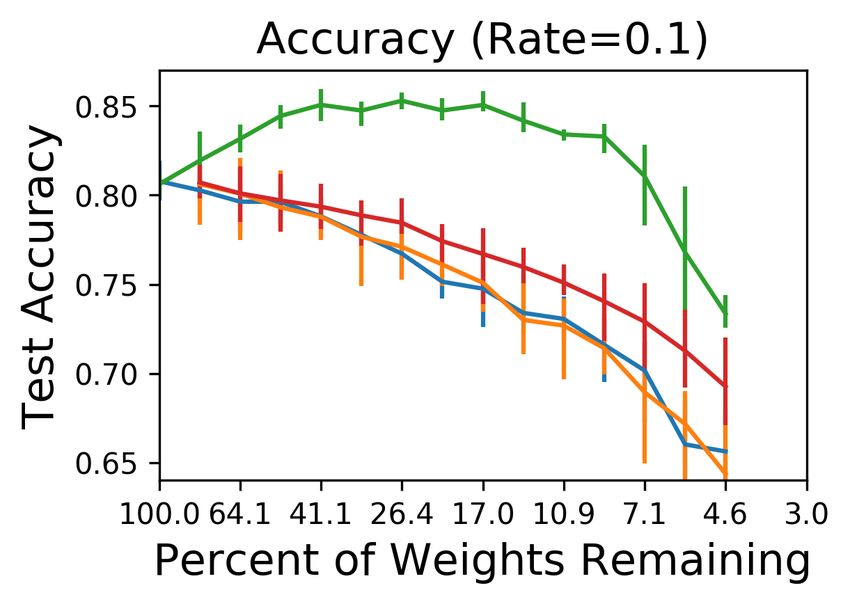
Figure 6(a): Resnet test accuracy as training proceeds. Figure 6(b): Resnet test accuracy averaged over the last
Percents are the fraction of weights remaining. Error 1,000 iterations of using the specified learning rate.
bars are elided for legibility.

both sets of benefits. Conv4 follows a similar pattern for accuracy. When pruned to between 16.2%
and 10.0%, average accuracy increases by more than 4 percentage points. Pruning the convolutional
layers alone to 7.3% causes average accuracy to rise by 5.8 percentage points.

4    Winning Tickets in Residual Networks

Here, we investigate the lottery ticket hypothesis as applied to residual networks, specifically
resnet18 [19] (see Figure 1) on CIFAR10. We match the training conditions of [19], with mini-batch
size 128, augmented data (random flips, translations), batch normalization, weight decay (0.0001),
and momentum (0.9). We follow a similar learning rate schedule: 0.1 for the first 20,000 iterations,
0.01 until iteration 25,000, and 0.001 to iteration 30,000. In this configuration, pruning does not
find winning tickets. Figure 6a, which plots test accuracy as the networks train, shows that the
network pruned to 32.9% converges more slowly to lower accuracy than the original. Figure 6b
(right) summarizes accuracy across all iterative winning ticket sizes. Pruning never improves the
accuracy of the network; its accuracy is no better than that of the randomly-reinitialized control trials.
However, when we use SGD without momentum, the usual lottery ticket pattern reemerges. The
average unpruned SGD-trained network’s accuracy is 89.1% as compared to 90.8% for the momentum-
trained network. However, when pruned to 32.9%, the average SGD-trained network initially learns
faster (Figure 6a) and reaches 90% accuracy. Winning tickets pruned by up to 83% surpass the
accuracy of the unpruned SGD-trained network; randomly-reinitialized controls follow the usual
pattern. Interestingly, the SGD-trained winning tickets outperform the momentum-trained network
by up to 4.5 percentage points (26.4% pruning) before the first learning rate change (Figure 6b left).
These results demonstrate that resnets can contain winning tickets. They also imply a nuanced
relationship between training strategies and our technique for finding winning tickets. It is possible
that training with momentum created a network for which pruning failed to find winning tickets, or
that the winning tickets it found could not train productively with momentum. Likewise, it is possible
that, had we custom-developed a learning schedule for the SGD-trained winning tickets, they might
have outperformed the momentum-trained network for the entirety of training.

5    Winning Tickets and Dropout

Dropout [48, 22] is a technique that improves network accuracy by randomly disabling a fraction of
the units (i.e., randomly sampling a subnetwork) on each training iteration. Baldi and Sadowski [3]
characterize dropout as simultaneously training the ensemble of all possible subnetworks. Since the
lottery ticket hypothesis suggests that one of these subnetworks comprises a winning ticket, it is
natural to ask whether dropout and our strategy for finding winning tickets interact.
Figure 7 shows the result of training the conv4 network with a dropout rate of 0.5 (orange). The blue
line is the baseline performance for conv4 (the same as the green line in Figure 4). When training
with dropout, we continue to identify winning tickets that converge faster than the unpruned network
(2.52x when pruned to 19.1%). Morever, these winning tickets reach higher accuracy; a winning
ticket pruned to 13.8% bests the accuracy of the unpruned dropout network by 5.5 percentage points
and the unpruned network without dropout by 9.6 percentage points.

                                                       6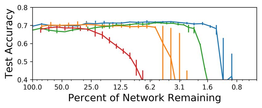
Figure 7: Convergence times and accuracies for dropout on conv4.

Figure 8: Histogram (normalized) of remaining initializations for each layer at four pruning levels.

These improvements suggest that the lottery ticket hypothesis continues to hold in the context of
dropout and, moreover, that the lottery ticket hypothesis and dropout may interact in a complementary
way. For example, Srivastava et al. [48] observed that dropout induces sparse activations in the
final network; it is possible that dropout-induced sparsity primes a network to be pruned. If this
is the case, dropout techniques that specifically target weights [49] or learn per-weight dropout
probabilities [38, 35] could make winning tickets even easier to find with our pruning-based method.

6   Examining Winning Tickets
In this section, we briefly examine the winning ticket initializations resulting from iteratively pruning
fully-connected networks trained on MNIST. Figure 8 shows the winning ticket initializations
(weights before training) at four levels of pruning. The left graph contains the initial truncated
normal distribution of weights in the unpruned network. To the right are the initial weights after
pruning to 51.3%. The initializations are the left and right extremes of the original distribution.
Nearly all weights that began near zero remained the smallest weights after training and were pruned
during the first few iterations; they were considered least important by our pruning heuristic, and the
network performed better without them. (The output layer maintains its structure for longer, likely
because we pruned it at a slower rate.) Han et al. [17] find this pattern for weights after training, but
Figure 8 shows that it originates before training. This pattern continues at 16.9% and 5.6%. While
these distributions differ significantly from typical initializations, these results suggest that randomly
initializing from a normal distribution may—in effect—sample a sparse architecture in which small
weights are infrequently part of winning tickets.

7   Related Work
In practice, neural networks tend to be dramatically over-parameterized. Distillation [2, 21] and
pruning [31, 17] rely on the fact that parameters can be reduced while preserving accuracy. Even with
sufficient capacity to memorize training data, networks naturally tend to learn simpler functions [51,
42, 1]. Contemporary experience [5, 21, 51] and our random reinitialization experiments suggest that
large networks are easier to train than small ones. Our contribution is to show that large networks
contain subnetworks capable of learning on their own starting from their original initializations.
Several other research directions aim to train small or sparse networks.

Prior to training. Squeezenet [25] and MobileNets [23] are specifically engineered image-
recognition networks that are an order of magnitude smaller than standard architectures. Denil
et al. [8] represent weight matrices as products of lower-rank factors. Li et al. [32] restrict optimiza-
tion to a small, randomly-sampled subspace of the parameter space (meaning all parameters can still
be updated); they successfully train networks under this restriction. We show that one need not even
update all parameters to optimize a network, and we find winning tickets though a principled search

                                                    7
process involving pruning. Our contribution to this class of approaches is to demonstrate that small,
trainable networks exist within larger networks in the form of winning tickets.
After training. Distillation [2, 21] trains small networks to mimic the behavior of large networks;
small networks are easier to train in this paradigm. Recent pruning work aims to compress large
models into forms that run with limited resources (e.g., on mobile devices). Although pruning is
central to our experiments, we aim to gain insight into why training needs the overparameterized
networks that make pruning necessary. LeCun et al. [31] and Hassibi et al. [18] first explored pruning
based on second derivatives. More recently, Han et al. [17, 15, 14] showed per-weight magnitude-
based pruning substantially reduces the size of image-recognition networks. Han et al. iteratively
train to convergence, prune, and continue training. Guo et al. [13] restore pruned connections as
they become relevant again. Han et al. [16] and Jin et al. [27] restore pruned connections to increase
network capacity after small weights have been pruned and surviving weights fine-tuned. Other
proposed pruning heuristics include pruning based on activations [24], redundancy [37, 44], per-
layer second derivatives [9], and energy/computation efficiency [50] (e.g., pruning convolutional
filters [33, 39, 36] or channels [20]). Cohen et al. [7] observe that convolutional filters are sensitive
to initialization (“The Filter Lottery”); after training, they randomly reinitialize unimportant filters.
During training. Bellac et al. [4] train with sparse networks and replace weights that reach zero
with new random connections. Srinivas et al. [47] and Louizos et al. [35] learn gating variables
that minimize the number of nonzero network parameters. Narang et al. integrate magnitude-
based pruning into training [40]. Gal and Ghahramani show that dropout approximates Bayesian
inference in Gaussian processes [10]. Bayesian perspectives on dropout learn the dropout probabilities
during training [11, 28, 46]. Techniques that learn per-weight, per-unit [46], or structured dropout
probabilities naturally [38, 41] or explicitly [34, 45] prune and sparsify networks during training
as dropout probabilities for some weights reach 1. In contrast, we train networks at least once to
find winning tickets. These techniques might also find winning tickets, or, by inducing sparsity, they
might beneficially interact with our methods for finding winning tickets (as discussed in Section 5).
8 Conclusions
We articulate the lottery ticket hypothesis to offer insight into why large networks are easier to train.
It states that, when training succeeds for a large network, a subnetwork (a winning ticket) has been
randomly initialized such that it can be trained in isolation to the same level of accuracy as the
original network in a comparable number of iterations. We showed that pruning naturally uncovers
winning tickets in fully-connected, convolutional, and residual networks, including when trained
with techniques like dropout and batch normalization. In nearly all cases, we could find winning
tickets that were more than 80% smaller than the original network. When pruned to moderate levels,
these winning tickets converged faster than the original network and reached higher accuracy. Both
initialization and structure play a role in the efficacy of these winning tickets. Based on these results,
we return to our motivating question and conjecture that large networks are easier to train because
they contain more combinations of subnetworks from which training can recover a winning ticket.
Limitations. We only consider vision-centric datasets and network architectures. We only show a
single method for finding winning tickets: pruning. We do not explain why the winning tickets we
find train effectively. Although we show that many networks contain winning tickets, we do not show
that containing a winning ticket is necessary or sufficient for a network to learn successfully.
Future directions. This paper documents empirical evidence for the lottery ticket hypothesis.
There are numerous opportunities to further understand and make practical use of this paradigm.
Examining winning tickets. Understanding the properties that make subnetworks winning tickets.
Training. Exploring the interaction between training strategies (e.g., momentum) and winning tickets.
Finding other winning tickets. Designing other strategies beyond pruning for finding winning tickets.
Improving training. Exploiting winning tickets to develop new network architectures and initialization
strategies. Modifying strategies that prune during training to explicitly search for winning tickets.
Theoretical foundations. Developing a formal understanding of the lottery ticket hypothesis.
8References
[1] Devansh Arpit, Stanisław Jastrz˛ebski, Nicolas Ballas, David Krueger, Emmanuel Bengio,
Maxinder S Kanwal, Tegan Maharaj, Asja Fischer, Aaron Courville, Yoshua Bengio, et al. 2017.
A Closer Look at Memorization in Deep Networks. In International Conference on Machine
Learning. 233–242.
[2] Jimmy Ba and Rich Caruana. 2014. Do deep nets really need to be deep?. In Advances in neural
information processing systems. 2654–2662.
[3] Pierre Baldi and Peter J Sadowski. 2013. Understanding dropout. In Advances in neural
information processing systems. 2814–2822.
[4] Guillaume Bellec, David Kappel, Wolfgang Maass, and Robert Legenstein. 2018. Deep
Rewiring: Training very sparse deep networks. Proceedings of ICLR (2018).
[5] Yoshua Bengio, Nicolas L Roux, Pascal Vincent, Olivier Delalleau, and Patrice Marcotte. 2006.
Convex neural networks. In Advances in neural information processing systems. 123–130.
[6] Nicholas Carlini and David Wagner. 2017. Towards evaluating the robustness of neural networks.
In Security and Privacy (SP), 2017 IEEE Symposium on. IEEE, 39–57.
[7] Joseph Paul Cohen, Henry Z Lo, and Wei Ding. 2016. RandomOut: Using a convolutional
gradient norm to win The Filter Lottery. ICLR Workshop (2016).
[8] Misha Denil, Babak Shakibi, Laurent Dinh, Nando De Freitas, et al. 2013. Predicting parameters
in deep learning. In Advances in neural information processing systems. 2148–2156.
[9] Xin Dong, Shangyu Chen, and Sinno Pan. 2017. Learning to prune deep neural networks
via layer-wise optimal brain surgeon. In Advances in Neural Information Processing Systems.
4860–4874.
[10] Yarin Gal and Zoubin Ghahramani. 2016. Dropout as a Bayesian approximation: Representing
model uncertainty in deep learning. In international conference on machine learning. 1050–
1059.
[11] Yarin Gal, Jiri Hron, and Alex Kendall. 2017. Concrete dropout. In Advances in Neural
Information Processing Systems. 3584–3593.
[12] Xavier Glorot and Yoshua Bengio. 2010. Understanding the difficulty of training deep feedfor-
ward neural networks. In Proceedings of the thirteenth international conference on artificial
intelligence and statistics. 249–256.
[13] Yiwen Guo, Anbang Yao, and Yurong Chen. 2016. Dynamic network surgery for efficient dnns.
In Advances In Neural Information Processing Systems. 1379–1387.
[14] Song Han, Huizi Mao, and William J. Dally. 2015. Deep Compression: Compressing Deep Neu-
ral Network with Pruning, Trained Quantization and Huffman Coding. CoRR abs/1510.00149
(2015). arXiv:1510.00149 http://arxiv.org/abs/1510.00149
[15] Song Han, Huizi Mao, and William J Dally. 2015. A deep neural network compression pipeline:
Pruning, quantization, huffman encoding. arXiv preprint arXiv:1510.00149 10 (2015).
[16] Song Han, Jeff Pool, Sharan Narang, Huizi Mao, Shijian Tang, Erich Elsen, Bryan Catanzaro,
John Tran, and William J Dally. 2017. Dsd: Regularizing deep neural networks with dense-
sparse-dense training flow. Proceedings of ICLR (2017).
[17] Song Han, Jeff Pool, John Tran, and William Dally. 2015. Learning both weights and con-
nections for efficient neural network. In Advances in neural information processing systems.
1135–1143.
[18] Babak Hassibi and David G Stork. 1993. Second order derivatives for network pruning: Optimal
brain surgeon. In Advances in neural information processing systems. 164–171.
9[19] Kaiming He, Xiangyu Zhang, Shaoqing Ren, and Jian Sun. 2016. Deep residual learning for
image recognition. In Proceedings of the IEEE conference on computer vision and pattern
recognition. 770–778.
[20] Yihui He, Xiangyu Zhang, and Jian Sun. 2017. Channel pruning for accelerating very deep
neural networks. In International Conference on Computer Vision (ICCV), Vol. 2. 6.
[21] Geoffrey Hinton, Oriol Vinyals, and Jeff Dean. 2015. Distilling the knowledge in a neural
network. arXiv preprint arXiv:1503.02531 (2015).
[22] Geoffrey E Hinton, Nitish Srivastava, Alex Krizhevsky, Ilya Sutskever, and Ruslan R Salakhut-
dinov. 2012. Improving neural networks by preventing co-adaptation of feature detectors. arXiv
preprint arXiv:1207.0580 (2012).
[23] Andrew G Howard, Menglong Zhu, Bo Chen, Dmitry Kalenichenko, Weijun Wang, Tobias
Weyand, Marco Andreetto, and Hartwig Adam. 2017. Mobilenets: Efficient convolutional
neural networks for mobile vision applications. arXiv preprint arXiv:1704.04861 (2017).
[24] Hengyuan Hu, Rui Peng, Yu-Wing Tai, and Chi-Keung Tang. 2016. Network trimming: A
data-driven neuron pruning approach towards efficient deep architectures. arXiv preprint
arXiv:1607.03250 (2016).
[25] Forrest N Iandola, Song Han, Matthew W Moskewicz, Khalid Ashraf, William J Dally, and
Kurt Keutzer. 2016. SqueezeNet: AlexNet-level accuracy with 50x fewer parameters and< 0.5
MB model size. arXiv preprint arXiv:1602.07360 (2016).
[26] Sergey Ioffe and Christian Szegedy. 2015. Batch normalization: Accelerating deep network
training by reducing internal covariate shift. arXiv preprint arXiv:1502.03167 (2015).
[27] Xiaojie Jin, Xiaotong Yuan, Jiashi Feng, and Shuicheng Yan. 2016. Training skinny deep neural
networks with iterative hard thresholding methods. arXiv preprint arXiv:1607.05423 (2016).
[28] Diederik P Kingma, Tim Salimans, and Max Welling. 2015. Variational dropout and the local
reparameterization trick. In Advances in Neural Information Processing Systems. 2575–2583.
[29] Alex Krizhevsky and Geoffrey Hinton. 2009. Learning multiple layers of features from tiny
images. (2009).
[30] Yann LeCun, Léon Bottou, Yoshua Bengio, and Patrick Haffner. 1998. Gradient-based learning
applied to document recognition. Proc. IEEE 86, 11 (1998), 2278–2324.
[31] Yann LeCun, John S Denker, and Sara A Solla. 1990. Optimal brain damage. In Advances in
neural information processing systems. 598–605.
[32] Chunyuan Li, Heerad Farkhoor, Rosanne Liu, and Jason Yosinski. 2018. Measuring the Intrinsic
Dimension of Objective Landscapes. Proceedings of ICLR (2018).
[33] Hao Li, Asim Kadav, Igor Durdanovic, Hanan Samet, and Hans Peter Graf. 2016. Pruning
filters for efficient convnets. arXiv preprint arXiv:1608.08710 (2016).
[34] Christos Louizos, Karen Ullrich, and Max Welling. 2017. Bayesian compression for deep
learning. In Advances in Neural Information Processing Systems. 3290–3300.
[35] Christos Louizos, Max Welling, and Diederik P Kingma. 2018. Learning Sparse Neural
Networks through L_0 Regularization. Proceedings of ICLR (2018).
[36] Jian-Hao Luo, Jianxin Wu, and Weiyao Lin. 2017. Thinet: A filter level pruning method for
deep neural network compression. arXiv preprint arXiv:1707.06342 (2017).
[37] Zelda Mariet and Suvrit Sra. 2016. Diversity networks. Proceedings of ICLR (2016).
[38] Dmitry Molchanov, Arsenii Ashukha, and Dmitry Vetrov. 2017. Variational dropout sparsifies
deep neural networks. arXiv preprint arXiv:1701.05369 (2017).
10[39] Pavlo Molchanov, Stephen Tyree, Tero Karras, Timo Aila, and Jan Kautz. 2016. Pruning convolu-
tional neural networks for resource efficient transfer learning. arXiv preprint arXiv:1611.06440
(2016).
[40] Sharan Narang, Erich Elsen, Gregory Diamos, and Shubho Sengupta. 2017. Exploring sparsity
in recurrent neural networks. Proceedings of ICLR (2017).
[41] Kirill Neklyudov, Dmitry Molchanov, Arsenii Ashukha, and Dmitry P Vetrov. 2017. Structured
bayesian pruning via log-normal multiplicative noise. In Advances in Neural Information
Processing Systems. 6778–6787.
[42] Behnam Neyshabur, Ryota Tomioka, and Nathan Srebro. 2014. In search of the real inductive
bias: On the role of implicit regularization in deep learning. arXiv preprint arXiv:1412.6614
(2014).
[43] Nicolas Papernot, Patrick McDaniel, Xi Wu, Somesh Jha, and Ananthram Swami. 2016. Distil-
lation as a defense to adversarial perturbations against deep neural networks. In Security and
Privacy (SP), 2016 IEEE Symposium on. IEEE, 582–597.
[44] Suraj Srinivas and R Venkatesh Babu. 2015. Data-free parameter pruning for deep neural
networks. arXiv preprint arXiv:1507.06149 (2015).
[45] Suraj Srinivas and R Venkatesh Babu. 2015. Learning neural network architectures using
backpropagation. arXiv preprint arXiv:1511.05497 (2015).
[46] Suraj Srinivas and R Venkatesh Babu. 2016. Generalized dropout. arXiv preprint
arXiv:1611.06791 (2016).
[47] Suraj Srinivas, Akshayvarun Subramanya, and R Venkatesh Babu. 2017. Training Sparse Neural
Networks. In Proceedings of the IEEE Conference on Computer Vision and Pattern Recognition
Workshops. 138–145.
[48] Nitish Srivastava, Geoffrey Hinton, Alex Krizhevsky, Ilya Sutskever, and Ruslan Salakhutdinov.
2014. Dropout: A simple way to prevent neural networks from overfitting. The Journal of
Machine Learning Research 15, 1 (2014), 1929–1958.
[49] Li Wan, Matthew Zeiler, Sixin Zhang, Yann Le Cun, and Rob Fergus. 2013. Regularization
of neural networks using dropconnect. In International Conference on Machine Learning.
1058–1066.
[50] Tien-Ju Yang, Yu-Hsin Chen, and Vivienne Sze. 2017. Designing energy-efficient convolutional
neural networks using energy-aware pruning. arXiv preprint (2017).
[51] Chiyuan Zhang, Samy Bengio, Moritz Hardt, Benjamin Recht, and Oriol Vinyals. 2016. Under-
standing deep learning requires rethinking generalization. arXiv preprint arXiv:1611.03530
(2016).
1110 Units 8 Units 6 Units 4 Units 2 Units
DB ZL DB ZL DB ZL DB ZL DB ZL
98.5 92.9 96.8 87.5 92.5 76.8 78.3 55.3 49.1 17.6
Figure 9: Success rates of 1000 random XOR networks, each with the specified number of hidden
units. DB = percent of trials that found the correct decision boundary. ZL = percent of trials that
reached zero loss.
Pruning Strategy 10 Units 4 Units (Pruned) 2 Units (Pruned)
DB ZL DB ZL DB ZL
One-shot Product 99.2 93.3 98.0 90.3 82.4 65.3
Input Magnitude 98.9 93.5 97.9 92.2 83.8 76.5
Output Magnitude 99.0 93.3 96.9 85.9 78.6 56.1
Product 98.5 92.9 97.6 90.3 91.5 79.4
Figure 10: Success rates of different pruning strategies on 1000 trials each. DB and ZL defined as in
Figure 9. The pruned columns include only those runs for which both the original ten-unit network
and the pruned winning ticket found the right decision boundary or reached zero loss. The first row
of the table was obtained by pruning in one shot; all subsequent rows involved pruning iteratively
A Winning Tickets and the XOR Function
Many of the same behaviors we observed in image-recognition networks also surface when learning
XOR with exceedingly simple networks.
The XOR function is among the simplest examples that distinguish neural networks from linear
classifiers. The XOR function has four data points: the coordinates (0, 0), (0, 1), (1, 0), and (1, 1).
The first and last points should be placed in class 0 and the middle two points in class 1. Geometrically,
this problem requires a nonlinear decision boundary. In this experiment, we consider the family of
fully connected networks for XOR with two input units, one hidden layer (ReLU activation), and one
output unit (sigmoid activation). Even with this simple level, the lottery ticket hypothesis surfaces.
Although a network of this form with two hidden units is sufficient to perfectly represent the
XOR function,3 the probability that a standard training approach—one that randomly initializes the
network’s weights and then applies gradient descent—correctly learns XOR for a network with two
hidden units is low relative to that for a larger network.
Figure 9 contains the overall success rates (percent of networks that found the right decision boundary
or reached zero loss). In 1000 training runs, a network with two hidden units learned a correct
decision boundary in only 49.1% of trials. Cross-entropy loss reached 0 (meaning the network
learned to output a hard 0 or 1) in only 17.6% of trials. Meanwhile, an otherwise identical network
outfitted with ten hidden units learned the decision boundary in 98.5% of trials and reached 0 loss in
92.9% of trials. Figure 9 charts the loss for these and other hidden layer sizes.4
To put the central question of this paper in the concrete terms of the XOR problem, why do we need
to start with a neural network with ten hidden units to ensure that training succeeds when a much
smaller neural network with two hidden units can represent the XOR function perfectly?
According to the lottery ticket hypothesis, successful networks with a large number of parameters
(e.g., the XOR network with ten hidden units) should contain winning tickets comprising a small
number of fortuitously-initialized weights on which training will still succeed.
3
n −n 1
Example satisfying weights for the first layer: −n n . Satisfying weights for the output unit: [ 1 ].
Satisfying bias for the output unit: −n/2. n ≥ 1. As n grows, the output approaches a hard 1 or 0.
4
Weights were sampled from a normal distribution centered at 0 with standard deviation 0.1; all values more
than two standard deviations from the mean were discarded and resampled. Biases were initialized to 0. The
network was trained for 10,000 iterations.
12A.1 Methodology
To test the lottery ticket hypothesis with the XOR function, we instantiated the experiment from Part
1 with the following details:
1. Randomly initialize a network with ten hidden units.
2. Train for 10,000 iterations on the entire training set.
3. Prune a certain number of hidden units according to a particular pruning heuristic.
4. To extract the winning ticket, reset the pruned network to the original initializations.
The first three steps extract the architecture of the winning ticket; the crucial final step extracts the
corresponding initializations. We ran this experiment with two different classes of pruning strategies.
One-shot pruning involves pruning the network in a single pass. For example, one-shot pruning
a network by 80% would involve removing 80% of its units after it has been trained. In contrast,
iterative pruning involves repeating steps (2) through (4) several times, removing a small portion of
the units (in our case, two units) on each iteration. We find iterative pruning to be more effective for
extracting smaller winning tickets; Han et al. [17] found the same for compressing large networks
while maintaining accuracy.
We consider three different heuristics for determining which hidden units should be pruned:
• Input magnitude: remove the hidden unit with the smallest average input weight magnitudes.
• Output magnitude: remove the hidden unit with the smallest output weight magnitude.
• Magnitude product: remove the hidden unit with the smallest product of the magnitude of
its output weight and the sum of the magnitudes of its input weights.
The magnitude product heuristic achieved the best results, so we use it unless otherwise stated.
A.2 Results
One-shot pruning. We generated 1000 networks with ten hidden units and pruned them down to
both four and two hidden units using the magnitude product heuristic. The results of doing so appear
in the first row of Figure 10. The winning tickets with two hidden units found the correct decision
boundary 82.4% of the time (up from 49.1% for randomly-initialized networks with two hidden units)
and reached zero loss 65.3% of the time (up from 17.6% of the time for a random network).
Iterative pruning. We conducted the iterative version of the pruning experiment 1000 times,
starting with networks containing ten hidden units that were eventually pruned down (in two unit
increments) to networks containing a candidate winning ticket of just two hidden units. Of the 93.5%
of ten hidden unit networks that reached zero loss, 84.9% 5 had a two hidden unit winning ticket
that also reached zero loss (as compared to 17.6% of randomly-intialized two hidden unit networks).
Likewise, of the 98.9% of ten hidden unit networks that found the correct decision boundary, 92.8%
had a two-unit winning ticket that did the same (as compared to 49.1% of randomly-initialized two
hidden unit networks). The four hidden unit winning tickets almost identically mirror the performance
of the original ten hidden unit network. They found the correct decision boundary and reached zero
loss respectively in 99% and 97% of cases where the ten hidden unit network did so. Both of these
pruned trials appear in Figure 10 (under the Magnitude Product row).
These experiments indicate that, although iterative pruning is more computationally demanding than
one-shot pruning, it finds winning tickets at a higher rate than one-shot pruning. More importantly,
they also confirm that networks with ten hidden units can be pruned down to winning tickets of two
hidden units that, when initialized to the same values as they were in the original network, succeed in
training far more frequently than a randomly initialized network with two hidden units. The winning
tickets with four hidden units succeed nearly as frequently as the ten unit networks from which
they derive. Both of these results support the lottery ticket hypothesis—that large networks contain
smaller, fortuitously-initialized winning tickets amenable to successful optimization.
5
These numbers are derived from the last row of Figure 10. 93.5% of networks with ten hidden units reached
zero loss. 79.4% of networks started with ten units, reached zero loss, and were pruned to into two-unit networks
that also reached zero loss. 79.4% of 93.5% is 84.9%.
13In addition to the magnitude-product pruning heuristic, we also tested the input magnitude and output
magnitude heuristics. The results of doing so appear in Figure 10. The magnitude product heuristic
outperformed both. We posit that this success is due to the fact that, in the XOR case when all
input values are either 0 or 1, the product of input and output weight magnitudes should mimic the
activation of the unit (and therefore with its influence on the output).
14You can also read