SQuantizer: Simultaneous Learning for Both Sparse and Low-precision Neural Networks
←
→
Page content transcription
If your browser does not render page correctly, please read the page content below
SQuantizer: Simultaneous Learning for
                                                                      Both Sparse and Low-precision Neural Networks

                                                                               Mi Sun Park            Xiaofan Xu       Cormac Brick
                                                                                                   Movidius, AIPG, Intel
                                                             mi.sun.park@intel.com, xu.xiaofan@intel.com, cormac.brick@intel.com
arXiv:1812.08301v2 [cs.CV] 23 Mar 2019

                                                                     Abstract                                          devices for real-time AI applications like intelligent cam-
                                                                                                                       eras, drones, autonomous driving, and augmented and vir-
                                             Deep neural networks have achieved state-of-the-art                       tual reality (AR/VR) in retail. To overcome this limitation,
                                         (SOTA) accuracies in a wide range of computer vision,                         academia and industry have investigated network compres-
                                         speech recognition, and machine translation tasks. How-                       sion and acceleration in various directions towards reducing
                                         ever the limits of memory bandwidth and computational                         complexity of networks, and made tremendous progresses
                                         power constrain the range of devices capable of deploy-                       in this area. It includes network pruning [8, 6, 31], network
                                         ing these modern networks. To address this problem, we                        quantization [20, 40, 2], low-rank approximation [30, 34],
                                         propose SQuantizer, a new training method that jointly op-                    efficient architecture design [27, 35], neural architecture
                                         timizes for both sparse and low-precision neural networks                     search [41, 5] and hardware accelerators [7, 23].
                                         while maintaining high accuracy and providing a high com-                         In this work, we focus on combining the two popular
                                         pression rate. This approach brings sparsification and low-                   network compression techniques of sparsification and quan-
                                         bit quantization into a single training pass, employing these                 tization into a single joint optimization training. In addi-
                                         techniques in an order demonstrated to be optimal.                            tion to reduce the training time by half, our method maxi-
                                             Our method achieves SOTA accuracies using 4-bit and                       mizes compression which is higher than applying either the
                                         2-bit precision for ResNet18, MobileNet-v2 and ResNet50,                      technique alone with SOTA accuracy, and further enables
                                         even with high degree of sparsity. The compression rates                      significant compute acceleration on deep neural networks
                                         of 18× for ResNet18 and 17× for ResNet50, and 9×                              (DNNs) hardware accelerators like Tensilica IP 2 and Sam-
                                         for MobileNet-v2 are obtained when SQuantizing1 both                          sung sparsity-aware Neural Porcessing Unit [28]. This is a
                                         weights and activations within 1% and 2% loss in accuracy                     key enabler of fast and energy efficient inference. As the
                                         for ResNets and MobileNet-v2 respectively. An extension of                    relative merits of sparsity and quantization are discussed in
                                         these techniques to object detection also demonstrates high                   Section 5, either the method alone can not provide optimal
                                         accuracy on YOLO-v3. Additionally, our method allows for                      performance. A few previous works [8, 19] applied both
                                         fast single pass training, which is important for rapid pro-                  the techniques one after the other to show that pruning and
                                         totyping and neural architecture search techniques.                           8-bit weight only quantization can work together to achieve
                                             Finally extensive results from this simultaneous training                 higher compression. However, applying one after the other
                                         approach allows us to draw some useful insights into the                      not only requires two-stage training, but also makes it dif-
                                         relative merits of sparsity and quantization.                                 ficult to quantize with lower precision after pruning, due to
                                                                                                                       the lack of understanding the impact of pruning weights on
                                                                                                                       quantization, and vice versa. We therefore aim for more
                                         1. Introduction                                                               efficient network training process with both sparse low-
                                                                                                                       precision weights and sparse low-precision activations.
                                            High-performing deep neural networks [10, 13, 27]
                                                                                                                           The main contributions of this work are summarized as
                                         consist of tens or hundreds of layers and have millions
                                                                                                                       below: (1) we propose a new training method to enable
                                         of parameters requiring billions of float point operations
                                                                                                                       simultaneous learning for sparse and low-precision neural
                                         (FLOPs). Despite the popularity and superior performance,
                                                                                                                       networks that sparsify and low-bit quantize both weights
                                         those high demands of memory and computational power
                                                                                                                       and activations. (2) we analyze the order effect of spar-
                                         make it difficult to deploy on resource-constrained edge
                                                                                                                       sification and quantization when trained together for opti-
                                           1 SQuantizing: joint optimization of Sparsification and low-precision

                                         Quantization.                                                                   2 https://ip.cadence.com/ai

                                                                                                                   1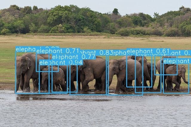
mal performance. (3) we extensively evaluate the effective-           with and without fine-tuning. Google Tensorflow Lite 3 and
ness of our approach on ImageNet classification task using            Nvidia TensorRT 4 support this functionality by importing
ResNet18, ResNet50 and MobileNet-v2, and also extend                  a pre-trained full-precision model and converting to 8-bit
to object detection task using YOLO-v3. The comparision               quantized model.
to prior quantization works shows that our method outper-                 Significant progress has recently been made on train-
forms across networks, even with additional high degree of            ing with quantization approach for low-precision networks
sparsity for further reduction in model size, memory band-            [38, 39, 36, 2, 37]. DoReFa-Net [38] presented a method to
width, energy and compute.                                            train CNNs that have low-precision weights and activations
                                                                      using low-precision parameter gradients. TTQ [39] intro-
2. Related Work                                                       duced a new training method for ternary weight networks
                                                                      with two learnable scaling coefficients for each layer. INQ
   Network Pruning: With a goal of easy deployment on                 [36] proposed an incremental training method of converting
embedded systems with limited hardware resources, sub-                pre-trained full-precision network into low-precision ver-
stantial efforts have been made to reduce network size by             sion with weights be either powers of two or zero. More
pruning redundant connections or channels from pre-trained            recent researches [20, 40, 3] have tackled the difficulty
models, and fine-tune to recover original accuracy. While             of training networks with both low-precision weights and
many of the related approaches differ in the method of de-            low-precision activations. Apprentice [20] used knowledge
termining the importance of weights or channels, the ba-              distillation technique by adding an auxiliary network to
sic goal of removing unimportant weights or channels from             guide for improving the performance of low-precision net-
original dense models to generate sparse or compact mod-              works. Low-bit CNN [40] presented three practical meth-
els remains the same. Specifically, fine-grained weight               ods of two-stage optimization, progressive quantization and
pruning (aka sparsification) [32, 8, 6, 29, 4] seeks to re-           guided training with full-precision network. PACT [3] pro-
move individual connections, while coarse-grained pruning             posed a new activation quantization function with a learn-
[12, 15, 17, 22, 33] seeks to prune entire rows/columns,              able parameter for clipping activations for each layer.
channels or even filters.
   Deep compression [8] introduced three-stage training               3. Our Method
of pruning, trained quantization and Huffman coding and
showed that weight pruning and weight quantization can                   In this section, we first introduce our SQuantizer for
work together for higher compression. Dynamic network                 simultaneous learning for sparse and low-precision neu-
surgery [6] presented an idea of connection splicing to re-           ral networks, and analyze the order effect of sparsification
store incorrectly pruned weights from the previous step.              and quantization techniques when trained together. Further-
Energy-aware pruning [32] proposed layer-by-layer energy-             more, we elaborate on the details of our sparsification and
aware weight pruning for energy-efficient CNNs that di-               quantization methods.
rectly uses the energy consumption of a CNN to guide the
                                                                      3.1. Learning both sparse and low-precision values
pruning process.
   ThiNet [15] presented a filter level pruning method for                Our proposed SQuantizer method is illustrated in Fig-
modern networks with consideration of special structures              ure 1. In each forward pass of training, we first sparsify
like residual blocks in ResNets. AMC [11] introduced Au-              full-precision weights based on a layer-wise threshold that
toML for structured pruning using reinforcement learning              is computed from the statistics of the full-precision weights
to automatically find out the effective sparsity for each layer       in each layer. Then, we quantize the non-zero elements of
and remove input channels accordingly. Generally speak-               the sparsified weights with min-max uniform quantization
ing, coarse-grained pruning results in more regular sparsity          function (i.e. The minimum and maximum values of the
patterns, making it easier for deployment on existing hard-           non-zero weights). In case of activation, prior sparsifica-
ware for speedup but more challenging to maintain original            tion is not necessary, since output activations are already
accuracy. On the other hand, fine-grained weight pruning              sparse due to the non-linearity of ReLU-like function. In
results in irregular sparsity patterns, requiring sparse matrix       general, ReLU activation function can result in about 50%
support but relatively easier to achieve higher sparsity.             sparsity. Therefore, we only quantize the output activations
   Network Quantization: Network quantization is an-                  after batch normalization and non-linearity, which is also
other popular compression technique to reduce the num-                the input activations to the following convolutional layer.
ber of bits required to represent each weight (or activation              In backward pass, we update the full-precision dense
value) in a network. Post-training quantization and training          weights with the gradients of the sparse and low-bit quan-
with quantization are two common approaches in this area.               3 https://www.tensorflow.org/lite/performance/
Post-training quantization is to quantize weights to 8-bit or         post_training_quantization
higher precision from a pre-trained full-precision network              4 https://developer.nvidia.com/tensorrt

                                                                  2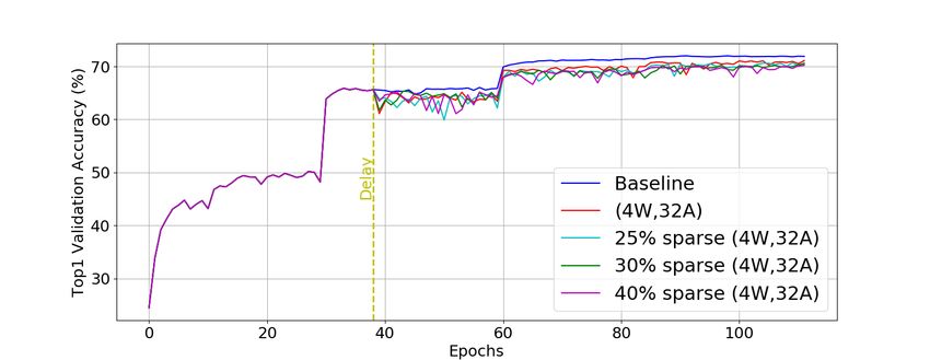
Convolution

        Layer (L-1)             Full Precision                    Sparse fp32
                                                                                                                                                             Layer L
 Activation Quantization        (fp32) Weight                       Weight                                                 Sparse Quantized
                                                                                                                                                    Activation Quantization
                                                                                                                             (SQ) Weight
                                                    Weight                        Weight
                                                 Sparsification                 Quantization

  0                        -1                       1        -1        0          1        -1         0         1         -W2 -W1   0 W1 W2          0
                                                                                                                                                             Loss

                                                                                                          Gradient

Figure 1. Overview of our proposed SQuantizer procedure for sparse and low-precision networks. The gray box shows the weight spar-
sification and quantization (SQuantization) steps in layer l in forward pass. The resulting sparse and low-bit quantized weights in layer l
are then convolved with low-bit quantized output activations of the previous layer l − 1. In backward pass, the full-precision weights are
updated with the gradients of SQuantized weights and activations at each iteration of training. Best view in color.

tized weights and activations. The gradients calculation for
the non-differential quantization function is approximated
with the straight-through estimator (STE) [1]. Our method
allows dynamic sparsification assignment and quantization
values by leveraging the statistics of the full-precision dense
weights in each iteration of training.
   After training, we discard the full-precision weights and
only keep the sparse and low-bit quantized weights to de-
ploy on resource-constrained edge devices. It is worth not-
ing that, in case of activation quantization, we still need to
perform on-the-fly quantization on output activations at in-                                   Figure 2. Weight histogram of ResNet56 layer3.5.conv2 layer on
ference time because it is dynamic depending on input im-                                      Cifar-10 using two different orders (S on Q and Q on S). X-axis
ages, unlike weights.                                                                          are weight values and Y-axis are frequency at log-scale.

                                                                                               tion, you may still utilize all the levels and in this case, the
3.2. Analysis of the order effect
                                                                                               order doesn’t matter. However, magnitude-based methods
   We analyze the order effect of the two compression                                          [9, 6, 31, 4] are commonly used and work better in practice.
(sparsification and quantization) techniques when applied                                      In fact, with Q on S, magnitude-based methods reduce the
together. Fundamentally, we want to find the optimal order                                     dynamic range of weights, thus reduce quantization error
that possibly leads to better performance. The two candi-                                      with finer quantization steps.
dates are quantization followed by sparsification (S on Q),
and sparsification followed by quantization (Q on S).                                          Table 1. Validation accuracy of sparse and 4-bit quantized
                                                                                               ResNet56 on Cifar-10 using two different orders (S on Q vs Q
   Figure 2 shows the weight histograms of layer3.5.conv2                                      on S). W and A represent weight and activation respectively.
layer (the last 3×3 convolutional layer in ResNet56) before
and after applying the two techniques based on the two dif-                                                                  S on Q                   Q on S
ferent orders. The top S on Q subfigure shows three his-                                                             Top1 (%) Sparsity (%)    Top1 (%) Sparsity (%)
                                                                                                     baseline         93.37          0         93.37         0
tograms of full-precision baseline, 4-bit quantized weights,                                    sparse (4W, 32A)      93.42         57         93.45         57
and sparse and 4-bit quantized weights (after sparsifying the                                   sparse (4W, 32A)      93.34         73         93.40         73
quantized weights) respectively. The bottom Q on S subfig-                                       sparse (4W, 4A)      92.88         57         92.94         57
ure represents the histograms of baseline, sparse weights,
and sparse and 4-bit quantized weights (after quantizing the                                      We also conduct experiments to verify our analysis with
sparsified weights) respectively.                                                              ResNet56 on Cifar-10, as shown in Table 1. As expected,
   It is observed from the histograms of S on Q, we don’t                                      Q on S consistently outperforms S on Q in all three exper-
fully utilize all quantization levels. Although we can use up                                  iments. Moreover, our sparse and 4-bit quantized models
to 24 levels for 4-bit quantization, we end up using fewer                                     give slightly better accuracy than the baseline, possibly be-
levels due to the subsequent sparsification. The higher                                        cause SQuantization acts as additional regularization which
sparsity, the more number of quantization levels will be                                       helps prevent overfitting. In summary, we believe that Q on
underutilized. Noting that this phenomenon heavily de-                                         S is more effective than S on Q, therefore we use Q on S in
pends on sparsification methods. With random sparsifica-                                       our SQuantizer.

                                                                                       3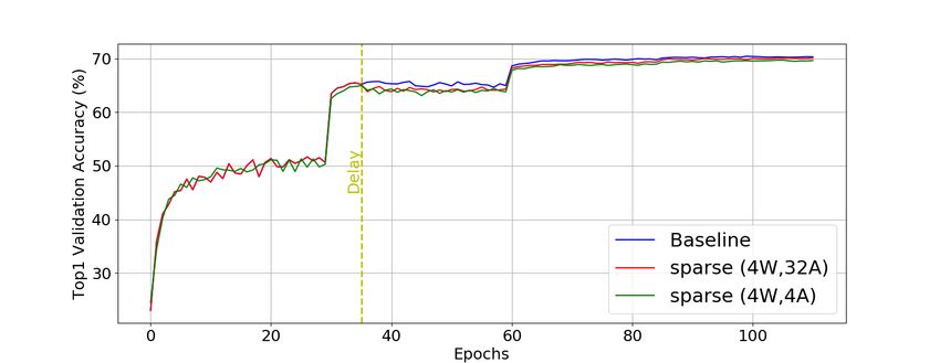
3.3. SQuantizer in details                                           Table 2. Effect of various σ on accuracy and sparsity of ResNet50
                                                                     on ImageNet. W represents weight.
3.3.1   Sparsification                                                                 Accuracy (%)                                 Compression
                                                                                                       Sparsity (%)   #Params (M)
                                                                                 σ     Top1    Top5                                    Rate
As shown in Figure 1, we first apply statistic-aware spar-            baseline         76.3    93.0         0              25.5          -
                                                                                 0.0   76.0    92.9        55              11.5        17×
sification to prune connections in each layer by remov-                          0.2   76.0    92.6        63               9.5        21×
                                                                        4W
ing (zeroing out) the connections with absolute weight val-                      0.4   75.4    92.5        69               7.9        25×
                                                                                 0.6   75.3    92.3        74               6.6        30×
ues lower than a layer-wise threshold. The basic idea                            0.0   74.8    92.2        56              11.3        36×
of statistic-aware sparsification is to compute a layer-wise            2W       0.1   74.6    92.1        59              10.4        39×
                                                                                 0.2   74.5    92.0        63               9.5        42×
weight threshold based on the current statistical distribution
of the full-precision dense weights in each layer, and mask
out weights that are less than the threshold in each forward
pass. In backward pass, we also mask out the gradients of
the sparsified weights with the same mask.
    We use layer-wise binary maskln (same size as weight
Wl ) for lth layer at nth iteration in Equation 1 and Equa-
   n

tion 2. Similar to [6, 31], this binary mask is dynamically
updated based on a layer-wise threshold and sparsity con-
trolling factor σ (same for all layers). The mean and one            Figure 3. σ vs sparsity of sparse and 4-bit ResNet50. X-axis is
standard deviation (std) of the full-precision dense weights         sigma (σ) and Y-axis is sparsity level (%).
in each layer are calculated to be a layer-wise threshold.
This allows previously masked out weights back if it be-             layer-wise pruning threshold tnl , while the max is the maxi-
comes more important (i.e. |Wln (i, j)| > tnl ). It should be        mum value of the sparse weights sparseWln in lth layer at
noted that our approach doesn’t need layer-by-layer prun-            nth iteration of training. Based on Equation 3 to Equation
ing [9, 32]. It globally prunes all layers with layer-wise           6, we quantize a full-precision non-zero element of sparse
thresholds considering different distribution of weights in          weight sparseWln (i, j) to k-bit wsq .
each layer. Our experiment shows that our statistics-aware
method performs better than globally pruning all layers with                     max = max(|sparseWln |),                  min = tnl         (3)
the same sparsity level, and is comparable to layer-by-layer
pruning with much less training epochs.
                                                                                                 |sparseWln (i,j)|−min
                          (                                                              ws =          max−min
                                                                                                                                             (4)
                            0 if |Wln (i, j)| < tnl
          maskln (i, j) =                                  (1)
                            1 if |Wln (i, j)| > tnl
                                                                                               1
                                                                                     wq =   2k−1 −1
                                                                                                    round((2k−1         − 1)ws )             (5)
           tnl   =   mean(|Wln |)   +   std(|Wln |)   ×σ   (2)
   Sparsity controlling factor σ is a hyper-parameter in this

statistic-aware pruning method. Unlike explicit level of tar-         wsq = sign(sparseWln (i, j)) wq (max − min) + min
get sparsity (i.e. prune 50% of all layers), σ is implicitly                                                                   (6)
determining sparsity level. To understand the effect of σ               In backward pass, in order to back-propagate the non-
on accuracy and sparsity level, we experiment for 4-bit and          differentiable quantization functions, we adopt the straight-
2-bit ResNet50 on ImageNet, shown in Table 2 and Figure              through estimator (STE) approach [1]. To be more specific,
3. As expected, the higher σ, the more sparsity we can get                                                 ∂w      ∂w
                                                                     we approximate the partial gradient ∂wqs and ∂wsqq with an
with a slight decrease in accuracy. We can achieve up to                                          ∂w                  ∂w
30× compression rate for sparse and 4-bit model within 1%            identity mapping, to be ∂wqs ≈ 1 and ∂wsqq ≈ 1 respectively.
drop in accuracy, while achieving up to 42× compression              In other words, we use the identity mapping to simply pass
rate for sparse and 2-bit model within 2% drop in accuracy.          through the gradient untouched to overcome the problem
                                                                     of the gradient of round() and sign() operations being zero
                                                                     almost everywhere.
3.3.2   Quantization
                                                                        For activation quantization, we use parameterized clip-
After masking out relatively less important weights, we              ping technique, PACT [3]. From our experiment, PACT [3]
quantize the non-zero elements of sparsified weights with            works better than static clipping to [0, 1] based activation
low-bitwidth k, as shown in Figure 1. For weight quantiza-           quantization methods [38, 40, 21]. On-the-fly activation
tion, we use min-max uniform quantization function with-             quantization at inference time has some minor costs and
out clipping to [-1, 1]. Our min is the previously determined        some significant benefits. Costs are scaling/thresholding at

                                                                 4
the accumulator output prior to re-quantization. A signifi- Algorithm 1 SQuantization for sparse and k-bit quantized
cant benefit is the reduction in data movement (and there- neural network
fore energy) required for activations, and a reduction in the Input:Training data; A random initialized full-precision
storage required for heap allocated activation maps. model{Wl : 1 6 l 6 L}; Weight SQuantization Delay;
Tying quantization methods to sparsity: Depending Sparsity controlling σ; Low-bitwidth k. Output: A sparse,
on quantization methods, there is a case that some weights k-bit quantized model{Wsparse,quantized,l : 1 6 l 6 L}
are quantized to zero giving free sparsity. For instance, 1: Step 1: Quantize Activation:
WRPN [21] quantizes small weights to 0 due to clipping to 2: for iter = 1, ..., Delay do
[-1, 1] with implicit min of 0 and max of 1, while DoReFa- 3: Randomly sample mini-batch data
Net [38] is not necessary to map the same small weights 4: Quantize activation based on parameterized clip-
to 0, due to prior tanh transformation before quantization. ping discussed in Section 3.3.2
Mainly due to the (disconnected) bi-modal distribution of 5: Calculate feed-forward loss, and update weights Wl
sparse weights, in Figure 2, we choose to use min-max 6: end for
quantization function to have finer quantization steps only 7: Step 2: SQuantize weights and activations to k-bit:
on non-zero elements of sparse weights which in turn re- 8: for iter = Delay, ..., T do
duce quantization error. Noting that our method is not gen- 9: Randomly sample mini-batch data
erating additional sparsity since the min value is always 10: With σ, calculate Wsparse,l based on tl by Equation
greater than zero and gets larger, as sparsity controlling σ 2 layer-wisely
becomes large. 11: With k, tl , Wsparse,l , calculate Wsparse,quantized,l
by Equation 3 to 6 layer-wisely
3.3.3 Overall Algorithm 12: Quantize activation based on parameterized clip-
ping discussed in Section 3.3.2
The procedure of our proposed SQuantizer is described in 13: Calculate feed-forward loss, and update weights Wl
Algorithm 1. Similar to [14], we introduce a Delay pa-
14: end for
rameter to set a delay for weight SQuantization. In other
words, we start quantizing activations but defer SQuantiz-
ing weights until Delay iterations to let weights stabilize
of 0.9 and weight decay of 1e−4 , and learning rate starting
at the start of training, thus converge faster. From our ex-
from 0.1 and divided by 10 at epochs 30, 60, 85, 100. Batch
periments, Delay of one third of total training iterations
size of 256 is used with maximum 110 training epochs. For
works well across different types of networks, and train-
evaluation, we first resize an image to 256×256 and use a
ing from scratch with Delay performs better than training
single center crop 224×224. Same as almost all prior works
without Delay. We believe the reason is because training
[38, 20, 40, 3], we don’t compress the first convolutional
from scratch with Delay allows enough time for weights to
(conv) and the last fully-connected (FC) layer, unless noted
stabilize and fully adapt the quantized activation.
otherwise. It has been observed that pruning or quantizing
the first and last layers degrade the accuracy dramatically,
4. Experiments but requires relatively less computation.
To investigate the performance of our proposed SQuan- For object detection task, we use open source PyTorch
tizer, we have conducted experiments on several popular version of YOLO-v35 with default hyper-parameters as our
CNNs for classification task using ImageNet dataset, and baseline and apply our SQuantizer on Darknet-53 backbone
even extended to object detection task using COCO Dataset. classifier for YOLO-v3.
In particular, we explore the following 4 representative net-
works to cover a range of different architectures: ResNet18 4.1. Evaluation on ImageNet
with basic blocks [10], pre-activation ResNet50 with bottle- We train and evaluate our model on ILSVRC2012 [26]
neck blocks [10], MobileNet-v2 [27] with depth-wise sep- image classification dataset (a.k.a. ImageNet), which in-
arable, inverted residual and linear bottleneck. Futhermore, cludes over 1.2M training and 50K validation images with
Darknet-53 for YOLO-v3 object detection [25]. 1,000 classes. We report experiment results of sparse 4-
Implementation details: We implemented SQuantizer bit quantized ResNet18, ResNet50 and MobileNet-v2, and
in PyTorch [24] and used the same hyper-parameters to train sparse 2-bit ResNet50, with comparison to prior works. It
different types of networks for ImageNet classification task. should be noted that almost all prior low-precision quantiza-
During training, we randomly crop 224×224 patches from tion works have not considered efficient network architec-
an image or its horizontal flip, and normalize the input with ture like MobileNet. We believe that, despite the difficulty,
per-channel mean and std of ImageNet with no additional
data augmentation. We use Nesterov SGD with momentum 5 https://github.com/ultralytics/yolov3
5our experiment on MobileNet-v2 will provide meaningful
insights on the trade-offs between accuracy and model size,
especially for severely resource-constrained edge devices.
4.1.1 Sparse and 4-bit quantized Networks
ResNet18: Table 3 shows the comparison of Top1 valida-
tion accuracy for 4-bit (both weight and activation) quan-
tized ResNet18 with prior works. Noting that the DoReFa-
Figure 4. Top1 validation accuracy vs epochs of sparse and 4-bit
Net [38] number is cited from PACT [3], and in the case ResNet18 on ImageNet. Best view in color.
of our -Quantizer6 , we set tnl to 0 in Equation 3 to disable
sparsification prior to quantization. Our SQuantizer outper-
forms the prior works, even with 57% of sparsity. Addition- publication. Our SQuantizer outperforms most of the prior
ally, our -Quantizer achieves the state-of-the-art accuracy of works, even with sparsity. However, although PACT [3]
4-bit ResNet18 without sparsification. shows better accuracy, its baseline accuracy is much higher
and still loses 0.4% accuracy after 4-bit quantization. Simi-
Table 3. Comparison of validation accuracy of 4-bit quantized larly, we also lose 0.4% accuracy after 4-bit SQuantization,
ResNet18 on ImageNet. W and A represent weight and activation with 41% sparsity (σ of -0.3 is applied).
respectively. From Table 5, it is observed that our SQuantizer with
DoReFa-Net∗ [38] PACT[3] Our -Quantizer Our SQuantizer
Top1 Top1 Top1 Top1 Sparsity (%)
41% sparsity gives almost as accurate as our -Quantizer. It
baseline 70.2 70.2 70.4 70.4 0 indicates that there is an effective value for sparsity control-
(4W, 4A) 68.1 69.2 69.7 69.4 57
ling σ for each network that allows optimal sparsity with no
In Table 4, our -Quantizer is used for dense and 4-bit to little loss in accuracy or even better accuracy due to ad-
models (4W, -A), while our SQuantizer with σ of 0 is ditional regularization. Automatically finding out the effec-
used for sparse and 4-bit quantized models (sparse (4W, - tive value for σ for each network will remain as our future
A)). When SQuantizing both weights and activations, we work. In practice, we first try with σ of 0 and then lower or
achieve up to 18× compression rate within 1% drop in ac- raise σ value according to the training loss in the first few
curacy. Due to the uncompressed last FC layer, the over- epochs, and estimate the corresponding final sparsity from
all sparsity is slightly lower than the conv sparsity (57% vs the intermediate model after step 1 in Algorithm 1.
60%). Table 5. SQuantization on ResNet50 on ImageNet
Table 4. SQuantization on ResNet18 on ImageNet Accuracy (%) Sparsity (%) Compression
#Params (M)
Top1 Top5 Conv All Rate
Accuracy (%) Sparsity (%) Compression baseline 76.3 93.0 0 0 25.5 -
#Params (M)
Top1 Top5 Conv All Rate (4W, 32A) 76.4 93.0 0 0 25.5 8×
baseline 70.4 89.7 0 0 11.7 - sparse (4W, 32A) 76.0 92.9 60 55 11.5 17×
(4W, 32A) 70.2 89.4 0 0 11.7 8× (4W, 4A) 76.0 92.7 0 0 25.5 8×
sparse (4W, 32A) 69.8 89.2 60 57 5.0 18× sparse (4W, 4A) 75.9 92.7 45 41 15.0 13×
(4W, 4A) 69.7 89.1 0 0 11.7 8× sparse (4W, 4A) 75.5 92.5 60 55 11.5 17×
sparse (4W, 4A) 69.4 89.0 60 57 5.0 18×
Table 5 and Table 2 show that within 1% accuracy drop,
Figure 4 plots Top1 validation accuracy over training we can achieve up to 17× compression rate for both weight
epochs for baseline, sparse 4-bit weights, and sparse 4-bit and activation SQuantization, and up to 30× compression
weights with 4-bit activations. The Delay in the plot is rate for weights only SQuantization. In addition, our -
where step 2 starts in Algorithm 1, and accuracy curves of Quantizer for 4-bit weights performs slightly better than the
baseline and sparse (4W, 32A), due to the same precision of baseline.
activation, are the same before Delay. Overall, the accu- MobileNet-v2: MobileNets are considered to be less at-
racy curve of our SQuantizer is similar to the baseline and tractive to network compression due to its highly efficient
shows some drop right after Delay of 35 epochs, but almost architecture, and as such present an ardent challenge to any
recovers back at the next lowering learning rate epoch (60 new network compression technique. To be more specific,
epochs). MobileNet-v2 uses 3× and 7× smaller number of parame-
ResNet50: We compare our SQuantizer for 4-bit ters than ResNet18 and ResNet50 respectively.
ResNet50 with many prior works in Table 6. Noting that Taking up this challenge, we applied our SQuantizer on
the DoReFa-Net [38] number is cited from PACT [3] and the latest MobileNet-v2 to further reduce model size and
Apprentice [20] number is directly from an author of the compared with prior work, in Table 7 and Table 9. Dif-
6 Our -Quantizer is used to represent the proposed SQuantizer with spar- ferent from other networks, we sparsify the last FC layer,
sification disabled. since the last FC layer alone uses about 36% of total param-
6Table 6. Comparison of validation accuracy of 4-bit quantized ResNet50 on ImageNet. W and A represent weight and activation respec-
tively.
DoReFa-Net∗ [38] Apprentice∗ [20] Low-bit CNN[40] PACT[3] Our -Quantizer Our SQuantizer
Top1 Top5 Top1 Top5 Top1 Top5 Top1 Top5 Top1 Top5 Top1 Top5 Sparsity (%)
baseline 75.6 92.2 76.2 - 75.6 92.2 76.9 93.1 76.3 93.0 76.3 93.0 0
(4W, 4A) 74.5 91.5 75.3 - 75.7 92.0 76.5 93.2 76.0 92.7 75.9 92.7 41
eters, while all conv layers consume about 63%, and the rest Table 9. SQuantization on MobileNet-v2 on ImageNet
Accuracy (%) Sparsity (%) Compression
of 1% is used in batch normalization. Table 7 shows that #Params (M)
Top1 Top5 Conv FC All Rate
our SQuantizer outperforms the prior work by large margin, baseline 72.0 90.4 0 0 0 3.6 -
(4W, 32A) 71.2 89.9 0 0 0 3.6 8×
even with sparsity. Additionally, our -Quantizer achieves sparse (4W, 32A) 70.7 89.5 21 32 25 3.1 9×
the state-of-the-art accuracy of 4-bit MobileNet-v2 without sparse (4W, 32A) 70.5 89.5 30 32 30 2.5 11×
sparse (4W, 32A) 70.2 89.3 35 51 40 2.1 13×
sparsification. (4W, 4A) 70.8 89.7 0 0 0 3.6 8×
sparse (4W, 4A) 70.3 89.5 21 32 25 3.1 9×
Table 7. Comparison of validation accuracy of 4-bit quantized
MobileNet-v2 on ImageNet. W and A represent weight and ac- 4.1.2 Sparse and 2-bit quantized Network
tivation respectively.
QDCN[16] Our -Quantizer Our SQuantizer We SQuantize both weight and activation for 2-bit
Top1 Top1 Top1 Sparsity (%) ResNet50, and compare with prior works in Table 8. The
baseline 71.9 72.0 72.0 0 table contains two different comparisons, without and with
(4W, 32A) 62.0 71.2 70.7 25 full-precision shortcut (fpsc). In the case of with fpsc, we
Table 9 shows that within 2% drop in accuracy, we can don’t SQuantize input activations and weights in the short-
achieve up to 13× compression rate for weight SQuantiza- cut (residual) path, as suggested by PACT-SWAB [2]. Also
tion, and up to 9× for both weight and activation SQuan- note that the DoReFa-Net [38] number is cited from Low-
tization. It is also observed that when applying our - bit CNN [40] and Apprentice [20] used 8-bit activation.
Quantizer for dense 4-bit weight model, it already lost 0.8% For 2-bit quantization, we slightly modified the min and
accuracy. For reference, ResNet18 lost 0.2% for the same max functions in Equation 3, for better performance. Ac-
configuration. As expected, the effect of quantization is cording to Equation 3, all non-zero weights are quantized
more significant on efficient network like MobileNet-v2. to either the smallest or largest values of non-zero weights
However, we believe this trade-offs between accuracy and with its own sign. To reduce the significant impact of largest
compression rate can help to determine the applicability of and smallest values, we use mean and std of non-zero ele-
deployment on severely resource-constrained edge devices. ments of sparse weights to determine new values of min and
max. To be specific, we use the mean of non-zero weights
as a value of new min and the sum of the mean and two std
as a value of new max. Then, we clamp the absolute values
of sparse weights with these new min and max.
As shown in Table 8, in the case of without fpsc, our
SQuantizer outperforms the prior works by large margin,
even with 40% sparsity. In the case of with fpsc, our SQuan-
tizer with 36% sparsity gives comparable performance con-
sidering that our baseline is (0.6%) lower but gives (0.3%)
smaller accuracy drop compared to PACT-SWAB [2]. Al-
Figure 5. Top1 validation accuracy vs epochs of sparse 4-bit
though we used σ of -0.3 for both the experiments, the spar-
MobileNet-v2 on ImageNet. Best view in color.
sity of the latter is lower due to uncompressed shortcut path.
Figure 5 plots Top1 validation accuracy over training
epochs for baseline, dense 4-bit weights, and sparse 4- From Table 2, it is already seen that for sparse and 2-bit
bit weights with various sparsity degree. At Delay of 38 weight ResNet50, we can achieve up to 42× compression
epochs, we start SQuantizing weights based on the same rate within 2% accuracy drop. It is worth noting that our
baseline with different configurations. It is seen that the SQuantizer neither demands an auxiliary network to guide
accuracy curves of sparse 4-bit models become less stable [20] nor require two-stage training [19] to achieve state-of-
with higher sparsity. Comparing to the dense 4-bit model, the-art accuracy for sparse and low-precision models.
we can have up to 40% sparsity within 1% drop in accu-
4.2. Extension to Object Detection
racy. It is worth noting that training with Delay allows us
to reuse the same intermediate model for experiments with We further applied our SQuantizer to object detection
different configurations and shortens training time. tasks using YOLO-v3 [25] on COCO dataset [18]. The
7Table 8. Comparison of validation accuracy of 2-bit quantized ResNet50 on ImageNet. W and A represent weight and activation respec-
tively. The last two works (PACT-SWAB∗ [2] and Our SQuantizer∗ ) use full-precision shortcut.
DoReFa-Net∗ [38] Apprentice[20] Low-bit CNN[40] PACT[3] Our SQuantizer PACT-SWAB∗ [2] Our SQuantizer∗
Top1 Top5 Top1 Top5 Top1 Top5 Top1 Top5 Top1 Top5 Sparsity (%) Top1 Top5 Top1 Top5 Sparsity (%)
baseline 75.6 92.2 76.2 - 75.6 92.2 76.9 93.1 76.3 93.0 0 76.9 - 76.3 93.0 0
(2W, 2A) 67.3 84.3 72.8(8bitAct) - 70.0 87.5 72.2 90.5 73.0 91.0 40 74.2(f psc) - 73.9(f psc) 91.6 36
dataset contains 80 classes and all the results are based on tions with 2-bit precision. Although the high (16×) com-
the images size of 416×416 pixels. pression rate is attractive, the degraded accuracy may not
The backbone of YOLO-v3 is Darknet-53 and similarly be acceptable for real-world applications. This motivated
as classification tasks, we did not perform SQuantizer on us to design a joint optimization technique for sparsity and
the first layer of the network.Training set-up are exactly the quantization, achieving maximal compression while keep-
same as the baseline training with initial learning rate of ing the accuracy close to the original model. As a result, we
1e−3 and divided by 10 at epoch 50. The σ of -0.1 and -0.3 achieve 17× compression for ResNet50 when SQuantizing
are used for 4-bit and 2-bit experiments respectively with both weights and activations with 4-bit precision and 41%
Delay at 20 epoch. The total number of training epochs is sparsity within 1% drop in accuracy. Table 11 shows reduc-
100 epoch which is the same as the baseline training time. tion in FLOPs when leveraging weight and activation spar-
Table 10. SQuantization on YOLO-v3 object detection with
sity of low-bit network. The baseline (the first row in Ta-
Darknet-53 on COCO Dataset with image size 416×416. ble 11) shows expected compute from existing hardwares,
while the rest rows show reduced compute when leveraging
Compression
mAP Sparsity (%) #Params (M)
Rate the sparsity from specialized sparse hardwares [28] (i.e. 5×
baseline 52.8 0 61.95 - reduction in FLOPs from 55% sparse 4-bit ResNet50).
sparse (4W, 32A) 52.0 55 28.08 17× Table 11. FLOPs for dense, 4-bit vs sparse, 4-bit ResNet50
sparse (2W, 32A) 50.3 46 33.63 29×
Weights FLOP Weight% Activation% FLOP%
dense (4W, 4A) 25.5M 7.7G 100 - 100
As shown in Table 10, our SQuantizer boost compres- dense (4W, 4A) 25.5M 3.2G 100 40.2 41.2
sion rate to 17× within 1 mAP drop from the baseline and 41% sparse (4W, 4A) 15.0M 1.9G 58.8 42.9 24.6
55% sparse (4W, 4A) 11.4M 1.3G 44.7 40.7 17.6
generate 55% sparsity. With SQuantizer for 2-bit weights,
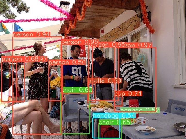
it gives 29× compression rate with 50.3 mAP. Moreover, Table12 shows potential benefits of our SQuantized
we show sample output images from the sparse and 4-bit model in terms of memory bandwidth, energy and computa-
quantized YOLO-v3 in Figure 6 for visual inspection. We tion. SQuantizer enables networks to fit in on-chip memory
believe this extension to object detection task demonstrates for embedded devices, which greatly reduces energy con-
the good general applicability of our proposed SQuantizer. sumption compared to fetching uncompressed weights from
an external DRAM. Hardware prototyping shows ∼2×
speedup per layer for ResNet50 with ∼50% sparsity.
Table 12. Potential benefits of compressed networks (W: weights,
A: activations)
Save Bandwidth? Save Energy? Save Compute?
Compress W X × ×
Skip computation cycles for either zero W or zero A X X X
Perform multiple lower-bitwidth operations together X X × (compute units X)
Figure 6. Output images from sparse and 4-bit quantized YOLO-
v3 with Darknet-53 as a backbone classifier. Best view in color.
6. Conclusion
In this paper, we proposed SQuantizer, a new training
5. Discussion method that enables simultaneous learning for sparse and
low-precision (weights and activations) neural networks,
Mathematically, for achieving 8× compression rate, we provides high accuracy and high compression rate. SQuan-
need to either quantize a model with 4-bit precision or spar- tizer outperforms across networks compared to the various
sify it with at least 87.5% sparsity level to have an equal rate prior works, even with additional sparsity. Furthermore, the
regardless of the storage overhead of non-zero elements in- extension to YOLO-v3 for object detection demonstrates
dices. From this calculation, we can infer that low-precision the viability and more general applicability of the proposed
(4-bit or lower) quantization can easily drive higher com- SQuantizer to broader vision neural network tasks. To the
pression rate than sparsification. However, prior works have best of our knowledge, this paper is the first approach to
shown that 2-bit or lower precision quantization results in demonstrating simultaneous learning for both sparse and
significant accuracy degradation. For example, the SOTA low-precision neural networks to help the deployment of
accuracy for ResNet50 (before our work) was 72.2% (4.7% high-performing neural networks on resource-constrained
drop) from [3], when quantizing both weights and activa- edge devices for real-world applications.
8References [16] R. Krishnamoorthi. Quantizing deep convolutional net-
works for efficient inference: A whitepaper. CoRR,
[1] Y. Bengio. Estimating or propagating gradients through abs/1806.08342, 2018.
stochastic neurons for conditional computation. arxiv
[17] H. Li, A. Kadav, I. Durdanovic, H. Samet, and H. P. Graf.
preprint arxiv:1308.3432.
Pruning filters for efficient convnets. CoRR, abs/1608.08710,
[2] J. Choi, P. I.-J. Chuang, Z. Wang, S. Venkataramani, V. Srini- 2016.
vasan, and K. Gopalakrishnan. Bridging the accuracy
[18] T.-Y. Lin, M. Maire, S. Belongie, J. Hays, P. Perona, D. Ra-
gap for 2-bit quantized neural networks (qnn). CoRR,
manan, P. Dollár, and C. L. Zitnick. Microsoft coco: Com-
abs/1807.06964, 2018.
mon objects in context. In European conference on computer
[3] J. Choi, Z. Wang, S. Venkataramani, P. I.-J. Chuang, V. Srini-
vision, pages 740–755. Springer, 2014.
vasan, and K. Gopalakrishnan. Pact: Parameterized clip-
ping activation for quantized neural networks. arXiv preprint [19] M. Mathew, K. Desappan, P. K. Swami, and S. Nagori.
arXiv:1805.06085, 2018. Sparse, quantized, full frame cnn for low power embedded
devices. In 2017 IEEE Conference on Computer Vision and
[4] T. Gale, E. Elsen, and S. Hooker. The state of sparsity in deep
Pattern Recognition Workshops (CVPRW), pages 328–336.
neural networks. arXiv preprint arXiv:1902.09574, 2019.
IEEE, 2017.
[5] A. Gordon, E. Eban, O. Nachum, B. Chen, T.-J. Yang, and
[20] A. Mishra and D. Marr. Apprentice: Using knowledge dis-
E. Choi. Morphnet: Fast & simple resource-constrained
tillation techniques to improve low-precision network accu-
structure learning of deep networks. CoRR, abs/1711.06798,
racy. In International Conference on Learning Representa-
2017.
tions, 2018.
[6] Y. Guo, A. Yao, and Y. Chen. Dynamic network surgery for
[21] A. Mishra, E. Nurvitadhi, J. J. Cook, and D. Marr. WRPN:
efficient dnns. In Advances In Neural Information Process-
Wide reduced-precision networks. In International Confer-
ing Systems, pages 1379–1387, 2016.
ence on Learning Representations, 2018.
[7] S. Han, X. Liu, H. Mao, J. Pu, A. Pedram, M. A. Horowitz,
and W. J. Dally. Eie: efficient inference engine on com- [22] P. Molchanov, S. Tyree, T. Karras, T. Aila, and J. Kautz.
pressed deep neural network. In Computer Architecture Pruning convolutional neural networks for resource efficient
(ISCA), 2016 ACM/IEEE 43rd Annual International Sympo- transfer learning. CoRR, abs/1611.06440, 2016.
sium on, pages 243–254. IEEE, 2016. [23] A. Parashar, M. Rhu, A. Mukkara, A. Puglielli, R. Venkate-
[8] S. Han, H. Mao, and W. Dally. Deep compression: Com- san, B. Khailany, J. Emer, S. W. Keckler, and W. J. Dally.
pressing deep neural networks with pruning, trained quanti- Scnn: An accelerator for compressed-sparse convolutional
zation and huffman coding, 10 2016. neural networks. In Proceedings of the 44th Annual Inter-
national Symposium on Computer Architecture, ISCA ’17,
[9] S. Han, J. Pool, J. Tran, and W. Dally. Learning both weights
pages 27–40, New York, NY, USA, 2017. ACM.
and connections for efficient neural network. In Advances
in neural information processing systems, pages 1135–1143, [24] A. Paszke, S. Gross, S. Chintala, G. Chanan, E. Yang, Z. De-
2015. Vito, Z. Lin, A. Desmaison, L. Antiga, and A. Lerer. Auto-
matic differentiation in pytorch. In NIPS-W, 2017.
[10] K. He, X. Zhang, S. Ren, and J. Sun. Deep residual learn-
ing for image recognition. In Proceedings of the IEEE con- [25] J. Redmon and A. Farhadi. Yolov3: An incremental improve-
ference on computer vision and pattern recognition, pages ment. arXiv preprint arXiv:1804.02767, 2018.
770–778, 2016. [26] O. Russakovsky, J. Deng, H. Su, J. Krause, S. Satheesh,
[11] Y. He, J. Lin, Z. Liu, H. Wang, L.-J. Li, and S. Han. Amc: S. Ma, Z. Huang, A. Karpathy, A. Khosla, M. Bernstein,
Automl for model compression and acceleration on mobile A. C. Berg, and L. Fei-Fei. ImageNet Large Scale Visual
devices. In Proceedings of the European Conference on Recognition Challenge. International Journal of Computer
Computer Vision (ECCV), pages 784–800, 2018. Vision (IJCV), 115(3):211–252, 2015.
[12] Y. He, X. Zhang, and J. Sun. Channel pruning for accelerat- [27] M. Sandler, A. Howard, M. Zhu, A. Zhmoginov, and L.-C.
ing very deep neural networks. In International Conference Chen. Mobilenetv2: Inverted residuals and linear bottle-
on Computer Vision (ICCV), volume 2, 2017. necks. In Proceedings of the IEEE Conference on Computer
[13] G. Huang, Z. Liu, L. van der Maaten, and K. Q. Weinberger. Vision and Pattern Recognition, pages 4510–4520, 2018.
Densely connected convolutional networks. In Proceedings [28] J. Song, Y. Cho, J.-S. Park, J.-W. Jang, S. Lee, J.-H. Song,
of the IEEE Conference on Computer Vision and Pattern J.-G. Lee, and I. Kang. An 11.5tops/w 1024-mac butterfly
Recognition, 2017. structure dual-core sparsity-aware neural processing unit in
[14] B. Jacob, S. Kligys, B. Chen, M. Zhu, M. Tang, A. Howard, 8nm flagship mobile soc. In IEEE International Solid-State
H. Adam, and D. Kalenichenko. Quantization and training Circuits Conference, pages 130–131. IEEE, 2019.
of neural networks for efficient integer-arithmetic-only in- [29] S. Srinivas and R. V. Babu. Data-free parameter pruning
ference. In The IEEE Conference on Computer Vision and for deep neural networks. arXiv preprint arXiv:1507.06149,
Pattern Recognition (CVPR), June 2018. 2015.
[15] J. W. Jian-Hao Luo and W. Lin. Thinet: A filter level prun- [30] C. Tai, T. Xiao, X. Wang, and W. E. Convolutional neu-
ing method for deep neural network compression. In ICCV, ral networks with low-rank regularization. arXiv preprint
pages 5058–5066, 2017. arXiv:1511.06067, 2015.
9[31] X. Xu, M. S. Park, and C. Brick. Hybrid pruning: Thinner
sparse networks for fast inference on edge devices. arXiv
preprint arXiv:1811.00482, 2018.
[32] T. Yang, Y. Chen, and V. Sze. Designing energy-efficient
convolutional neural networks using energy-aware pruning.
In 2017 IEEE Conference on Computer Vision and Pattern
Recognition (CVPR), pages 6071–6079, July 2017.
[33] J. Ye, X. Lu, Z. Lin, and J. Z. Wang. Rethinking the
smaller-norm-less-informative assumption in channel prun-
ing of convolution layers. arXiv preprint arXiv:1802.00124,
2018.
[34] X. Yu, T. Liu, X. Wang, and D. Tao. On compressing deep
models by low rank and sparse decomposition. In 2017
IEEE Conference on Computer Vision and Pattern Recog-
nition (CVPR), pages 67–76, July 2017.
[35] X. Zhang, X. Zhou, M. Lin, and J. Sun. Shufflenet: An
extremely efficient convolutional neural network for mobile
devices. arXiv preprint arXiv:1707.01083, 2017.
[36] A. Zhou, A. Yao, Y. Guo, L. Xu, and Y. Chen. Incremen-
tal network quantization: Towards lossless cnns with low-
precision weights. arXiv preprint arXiv:1702.03044, 2017.
[37] A. Zhou, A. Yao, K. Wang, and Y. Chen. Explicit loss-error-
aware quantization for low-bit deep neural networks. In Pro-
ceedings of the IEEE Conference on Computer Vision and
Pattern Recognition, pages 9426–9435, 2018.
[38] S. Zhou, Y. Wu, Z. Ni, X. Zhou, H. Wen, and Y. Zou.
Dorefa-net: Training low bitwidth convolutional neural
networks with low bitwidth gradients. arXiv preprint
arXiv:1606.06160, 2016.
[39] C. Zhu, S. Han, H. Mao, and W. J. Dally. Trained ternary
quantization. arXiv preprint arXiv:1612.01064, 2016.
[40] B. Zhuang, C. Shen, M. Tan, L. Liu, and I. Reid. Towards
effective low-bitwidth convolutional neural networks. In The
IEEE Conference on Computer Vision and Pattern Recogni-
tion (CVPR), June 2018.
[41] B. Zoph and Q. V. Le. Neural architecture search with rein-
forcement learning. 2017.
10You can also read