Expectations on mass determination using astrometric
←
→
Page content transcription
If your browser does not render page correctly, please read the page content below
A&A 640, A83 (2020)
https://doi.org/10.1051/0004-6361/201937061                                                                            Astronomy
c ESO 2020                                                                                                              &
                                                                                                                       Astrophysics

              Expectations on mass determination using astrometric
                            microlensing by Gaia ? , ??
                                              J. Klüter1 , U. Bastian1 , and J. Wambsganss1,2

      1
          Zentrum für Astronomie der Universität Heidelberg, Astronomisches Rechen-Institut, Mönchhofstr. 12-14, 69120 Heidelberg,
          Germany
          e-mail: klueter@ari.uni-heidelberg.de
      2
          International Space Science Institute, Hallerstr. 6, 3012 Bern, Switzerland

      Received 5 November 2019 / Accepted 28 April 2020

                                                                    ABSTRACT

      Context. Astrometric gravitational microlensing can be used to determine the mass of a single star (the lens) with an accuracy of a
      few percent. To do so, precise measurements of the angular separations between lens and background star with an accuracy below
      1 milli − arcsec at different epochs are needed. Therefore only the most accurate instruments can be used. However, since the timescale
      is on the order of months to years, the astrometric deflection might be detected by Gaia, even though each star is only observed on a
      low cadence.
      Aims. We want to show how accurately Gaia can determine the mass of the lensing star.
      Methods. Using conservative assumptions based on the results of the second Gaia data release (Gaia DR2), we simulated the indi-
      vidual Gaia measurements for 501 predicted astrometric microlensing events during the Gaia era (2014.5–2026.5). For this purpose
      we used the astrometric parameters of Gaia DR2, as well as an approximative mass based on the absolute G magnitude. By fitting
      the motion of the lens and source simultaneously, we then reconstructed the 11 parameters of the lensing event. For lenses passing by
      multiple background sources, we also fitted the motion of all background sources and the lens simultaneously. Using a Monte-Carlo
      simulation we determined the achievable precision of the mass determination.
      Results. We find that Gaia can detect the astrometric deflection for 114 events. Furthermore, for 13 events Gaia can determine the
      mass of the lens with a precision better than 15% and for 13 + 21 = 34 events with a precision of 30% or better.
      Key words. astrometry – gravitational lensing: micro – stars: low-mass – catalogs – proper motions – white dwarfs

1. Introduction                                                              OGLE2 (Udalski 2003). By using the OGLE data in combina-
                                                                             tion with simultaneous observations from the Spitzer telescope,
The mass is the most substantial parameter of a star. It defines             it was possible to determine the mass of a few isolated objects
its temperature, surface gravity, and evolution. Currently, rela-            (e.g. Zhu et al. 2016; Chung et al. 2017; Shvartzvald et al. 2019;
tions concerning stellar mass are based on binary stars, where a             Zang et al. 2020), whereas the astrometric shift of the source
direct mass measurement is possible (Torres et al. 2010). How-               was detected for the first time only recently (Sahu et al. 2017;
ever, it is known that single stars evolve differently. Hence it is          Zurlo et al. 2018). Especially Sahu et al. (2017) showed the
important to derive the masses of single stars directly. Apart from          potential of astrometric microlensing to measure the mass of
strongly model-dependent asteroseismology, microlensing is the               a single star with a precision of a few percent (Paczyński
only usable tool. It can be applied either by observing astromet-            1995). However, even though astrometric microlensing events
ric microlensing events (Paczyński 1991, 1995) or by detecting              are much rarer than photometric events, they can be pre-
finite source effects in photometric microlensing events and mea-            dicted from stars with known proper motions. The first sys-
suring the microlens parallax (Gould 1992). As a sub-area of                 tematic search for astrometric microlensing events was done
gravitational lensing, which was first described by Einstein’s the-          by Salim & Gould (2000). Using the first data release of the
ory of general relativity (Einstein 1915), microlensing describes            Gaia mission (Gaia Collaboration 2016), McGill et al. (2018)
the time-dependent positional deflection (astrometric microlens-             predicted one event caused by a nearby white dwarf. Cur-
ing) and magnification (photometric microlensing) of a back-                 rently, precise predictions (e.g. Klüter et al. 2018a,b; Bramich
ground source by an intervening stellar mass. Up to now, pho-                2018; Mustill et al. 20183 ; Bramich & Nielsen 2018) make use
tometric magnification was almost exclusively monitored and                  of Gaia’s second data release (Gaia DR2; Gaia Collaboration
investigated by surveys such as MOA1 (Bond et al. 2001) or                   2018) or even combine Gaia DR2 with external catalogues (e.g.
                                                                             Nielsen & Bramich 2018; McGill et al. 2019).
  ?
    The results for all simulated events, including Tables A.1 and A.2 are
only available at the CDS via anonymous ftp to cdsarc.u-strasbg.fr
(130.79.128.5) or via http://cdsarc.u-strasbg.fr/viz-bin/
                                                                             2
cat/J/A+A/640/A83                                                              Optical Gravitational Lensing Experiment.
 ??                                                                          3
    The Python-based code for our simulation is made publicly avail-           Mustill et al. (2018) searched for photometric micolensing events,
able at https://github.com/jkluter/MLG.                                      however, for all of their predicted events a measurable deflection is also
1
   Microlensing Observations in Astrophysics.                                expected.

                                                         Article published by EDP Sciences                                          A83, page 1 of 14
A&A 640, A83 (2020)

     The timescales of astrometric microlensing events are typ-
ically longer than the timescales of photometric events (a few
months instead of a few weeks; Dominik & Sahu 2000). Hence,
they might be detected and characterised by Gaia alone, even
though Gaia observes each star only occasionally. The Gaia mis-
sion of the European Space Agency (ESA) is currently the most
precise astrometric survey. Since mid-2014 Gaia has observed
the full sky with an average of about 70 measurements within
the nominal five years mission. Gaia DR2 contains only a sum-
mary of results from the data analysis (J2015.5 position, proper
motion, parallax, etc.) of its 1.6 billion stars, based on the first
approximately two years of observations. However, with the
fourth data release (expected in 2024) and the final data release
after the end of the extended mission, individual Gaia mea-
surements will also be published. Using these measurements, it
should be possible to determine the masses of individual stars
using astrometric microlensing. This will lead to a better under-
standing of mass relations for main sequence stars (Paczyński
1991).
     In the present paper we show the potential of Gaia to deter-
mine stellar masses using astrometric microlensing. We do so
by simulating the individual measurements for 501 predicted             Fig. 1. Astrometric shift for an event with an Einstein radius of θE =
microlensing events caused by 441 different stars. We also show         12.75mas (black circle) and an impact parameter of u = 0.75. While
the potential of combining the data for multiple microlensing           the lens (red) passes a background star (black star, fixed in origin) two
events caused by the same lens.                                         images (blue dashed, major image + and minor image – ) of the source
     In Sect. 2 we describe astrometric microlensing. In Sect. 3        are created due to gravitational lensing. This leads to a shift in the cen-
we explain in brief the Gaia mission and satellite, with a focus        tre of light, shown in green. The straight long-dashed black line con-
                                                                        nects the positions of the images for one epoch. While the lens moves
on important aspects for this paper. In Sect. 4 we show our             in the direction of the red arrow, all other images move according to
analysis, starting with the properties of the predicted events in       their individual arrows. The red, blue, and green dots correspond to dif-
Sect. 4.1, the simulation of the Gaia measurements in Sect. 4.2,        ferent epochs with fixed time steps (after Proft et al. 2011).
the fitting procedure Sect. 4.3, and finally the statistical analy-
sis in Sect. 4.4. In Sect. 5 we present the opportunities for direct
stellar mass determinations by Gaia. Finally, we summarise the          with u = |u|.
simulations and results and present our conclusions in Sect. 6.            For the unresolved case, only the centre of light of both
                                                                        images can be observed. This can be expressed by (Hog et al.
                                                                        1995; Miyamoto & Yoshii 1995; Walker 1995)
2. Astrometric microlensing
The positional change in the centre of light of the background                 A+ θ+ + A− θ− u2 + 3
                                                                        θc =                = 2     u · θE ,                                   (3)
star (“source”) due to the gravitational deflection of a passing                 A+ + A−     u +2
foreground star (“lens”) is called astrometric microlensing. This
is shown in Fig. 1. While the lens is passing the source, two           where A± are the magnifications of the two images given by
images of the source are created: a bright major image (+) close        (Paczyński 1986)
to the unlensed position, and a faint minor image (−) close to the
lens. In a case of perfect alignment, both images merge to an                      u2 + 2
Einstein ring, with a radius of (Chwolson 1924; Einstein 1936;          A± =       √       ± 0.5·                                              (4)
                                                                                 2u u2 + 4
Paczyński 1986)
                                        s                               The corresponding angular shift is given by
         4GML DS − DL                     ML $L − $S
      r
θE =                      = 2.854 mas          ·          ,    (1)                 u
           c2 DS · DL                     M       1 mas                 δθ c =          · θE .                                                 (5)
                                                                                 u2 + 2
where ML is the mass of the lens, DL , DS are the distances of
the lens and source from the observer, and $L ,$S are the paral-        The measurable deflection can be further reduced due to
laxes of lens and source, respectively. The gravitational constant      luminous-lens effects. However, in the following, we consider
is G and c is the speed of light. For a solar-type star at a distance   the resolved case where luminous-lens effects can be ignored.
of about 1 kiloparsec the Einstein radius is of the order of a few      Due to Eqs. (2) and (4), the influence of the minor image can
milli-arc-seconds (mas). The Einstein radius defines the angu-          only be observed when the impact parameter is of the same order
lar scale of the microlensing event. Using the unlensed scaled          of magnitude as, or smaller than, the Einstein radius. There-
angular separation on the sky u = ∆φ/θE , where ∆φ is the two-          fore the minor image is difficult to resolve and so far has been
dimensional unlensed angular separation, the position of the two        resolved only once (Dong et al. 2019). Hence, the observable for
lensed images can be expressed as a function of u, by (Paczyński       the resolved case is only the shift of the position of the major
1996)                                                                   image. This can be expressed by
           √
                                                                                      (u2 + 4) − u u
                                                                                  p
      u ± u2 + 4 u
θ± =                · · θE ,                                      (2)   δθ+ =                     · · θE ·                                     (6)
            2         u                                                                   2        u
A83, page 2 of 14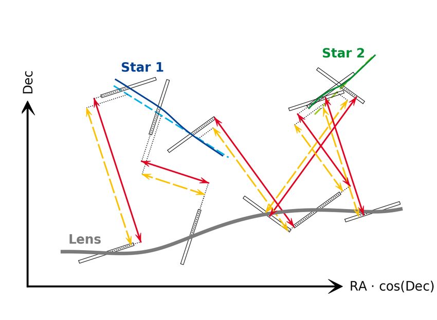
J. Klüter et al.: Expectations on mass determination using astrometric microlensing by Gaia

For large impact parameters u  5 this can be approximated as
(Dominik & Sahu 2000)

        θE   θ2   ML
δθ+ '      = E ∝      ,                                         (7)
         u  |∆φ| |∆φ|
which is proportional to the mass of the lens. Nevertheless
Eq. (5) is also a good approximation for the shift of the major
image whenever u > 5, since then the second image is negligi-
bly faint. This is always the case in the present study.

3. Gaia satellite
The Gaia satellite is a space telescope of the ESA that was
launched in December 2013. It is located at the Earth-Sun
Lagrange point L2, where it orbits the sun at roughly a 1% greater
distance than the earth. In mid 2014 Gaia started to observe the
whole sky on a regular basis defined by a nominal (pre-defined)
scanning law.

3.1. Scanning law                                                      Fig. 2. Illustration of the readout windows. For the brightest source (big
                                                                       blue star) Gaia assigns the full window (blue grid) of 12 × 12 pixels.
The position and orientation of Gaia is defined by various peri-       When a second source is within this window (e.g. red star) we assume
odic motions. First, it rotates on its own axis with a period of       that this star is not observed by Gaia. If the brightness of both stars is
six hours. Second, Gaia’s spin axis is inclined by 45 degrees          similar (∆G < 1 mag) we also neglect the brighter source. For a sec-
to the sun, with a precession frequency of one turn around             ond source close by but outside of the readout window (e.g. grey star)
the sun every 63 days. Finally, Gaia is not fixed at L2 but            Gaia assigns a truncated readout window (green grid). We assume that
                                                                       this star can be observed, and the precision along the scan direction is
moves on a 100 000 km Lissajous-type orbit around L2. The
                                                                       the same as for the full readout window. For more distant sources (e.g.
orbit of Gaia and the inclination is chosen such that the over-        yellow star) Gaia assigns a full window.
all coverage of the sky is quite uniform, with about 70 obser-
vations per star during the nominal five-year mission (2014.5
to 2019.5 Gaia Collaboration 2016) in different scan angles.           simulations, we stack the data of these eight or nine CCDs into
However, certain parts of the sky are inevitably observed more         one measurement. Finally, the source passes a red and blue pho-
often. Consequently, Gaia cannot be pointed at a certain tar-          tometer, plus a radial-velocity spectrometer (Gaia Collaboration
get at a given time. We used the Gaia observation forecast tool        2016). In order to reduce the volume of data, only small “win-
(GOST)4 to gather information on when a target is inside the           dows” around detected sources are read out and transmitted to
field of view of Gaia, and the current scan direction of Gaia          ground. For faint sources (G > 13 mag) these windows are
at each of those times. The GOST also lists the charge-coupled         12 × 12 pixels (along − scan × across − scan). This corresponds
device (CCD) row, which can be translated into eight or nine           to 708 mas × 2124 mas, due to a 1:3 pixel-size ratio. These data
CCD observations. More details on the scanning law can be              are stacked by the onboard processing of Gaia in an across-
found in Gaia Collaboration (2016) or the Gaia Data Release            scan direction into a one-dimensional strip, which is then trans-
Documentation5 .                                                       mitted to Earth. For bright sources (G < 13 mag), larger win-
                                                                       dows (18 × 12 pixel) are read out. These data are transferred
                                                                       as 2D images (Carrasco et al. 2016). When two sources with
3.2. Focal plane and readout window
                                                                       overlapping readout windows (e.g. Fig. 2) are detected, Gaia’s
Gaia is equipped with two separate telescopes with rectangu-           onboard processing assigns the full window to only one of the
lar primary mirrors, pointing at two fields of view, separated         sources (usually the brighter source). For the second source,
by 106.5◦ . This results in two observations only a few hours          Gaia assigns only a truncated window. For Gaia DR2 these trun-
apart with the same scanning direction. The light of the two           cated windows are not processed6 . More details on the focal
fields of view is focused on one common focal plane that is            plane and readout scheme can be found in Gaia Collaboration
equipped with 106 CCDs arranged in seven rows. The major-              (2016).
ity of the CCDs (62) are used for the astrometric field. While
Gaia rotates, the source first passes a sky mapper, which can dis-     3.3. Along-scan precision
tinguish between both fields of view. Afterwards, it passes nine
CCDs of the astrometric field (or eight for the middle row). The       Published information about the precision and accuracy of Gaia
astrometric field is devoted to position measurements, providing       mostly refers to the end-of-mission standard errors, which result
the astrometric parameters, and also G-band photometry. For our        from a combination of all individual measurements and also con-
                                                                       sider the different scanning directions. Gaia DR1 provides an
4
  Gaia observation forecast tool,                                      analytical formula to estimate this precision as a function of G
https://gaia.esac.esa.int/gost/.
5                                                                      6
  Gaia Data Release Documentation – The scanning law in theory           Gaia Data Release Documentation – Data model description
https://gea.esac.esa.int/archive/documentation/GDR2/                   https://gea.esac.esa.int/archive/documentation/GDR2/
Introduction/chap_cu0int/cu0int_sec_mission/cu0int_                    Gaia_archive/chap_datamodel/sec_dm_main_tables/ssec_
ssec_scanning_law.html.                                                dm_gaia_source.html.

                                                                                                                              A83, page 3 of 14
A&A 640, A83 (2020)
Fig. 4. Illustration of our simulation. While the lens (thick grey line)
passes the background star 1 (dashed blue line) the observed position of
the background star is slightly shifted due to microlensing (solid blue
line). The Gaia measurements are indicated as black rectangles, where
the precision in the along-scan direction is much better than the preci-
Fig. 3. Precision in along-scan direction as function of G magnitude. sion in the across-scan direction. The red arrows indicate the along-scan
The red line indicates the expected formal precision from Gaia DR2 for separation including microlensing, and the yellow dashed arrows show
one CCD observation. The blue solid line is the actually achieved preci- the along-scan separation without microlensing. The difference between
sion (Lindegren et al. 2018). The light blue dashed line shows the rela- both sources shows the astrometric microlensing signal. Due to the dif-
tion for the end-of-mission parallax error (Gaia Collaboration 2016), ferent scaning direction, an observation close to the maximal deflection
and the green dotted line shows the adopted relation for the precision of the microlensing event does not necessarily have the largest signal.
per CCD observation for the present study. The adopted precision for A further background star 2 (green) can improve the result.
nine CDD observations is shown as a thick yellow curve. The inlay (red
and blue curve) is taken from Lindegren et al. (2018), Fig. 9.
We also included the events outside the most extended mission
magnitude and V–I colour (Gaia Collaboration 2016). However, of Gaia (ending in 2024.5), since it is possible to determine the
we are interested in the precision of one single field-of-view scan mass only from the tail of an event (e.g. event #62 – #65 in
(i.e. the combination of the eight or nine CCD measurements in Table A.2), or from using both Gaia measurements and addi-
the astrometric field). The red line in Fig. 3 shows the formal pre- tional observations. The sample is naturally divided into two cat-
cision in the along-scan direction for one CCD (Lindegren et al. egories: events where the motion of the background source is
2018). The precision is mainly dominated by photon noise. Due known, and events where the motion of the background source
to different readout gates, the number of photons is roughly con- is unknown. A missing proper motion in Gaia DR2 will not
stant for sources brighter than G = 12 mag. The blue line in automatically mean that Gaia cannot measure the motion of
Fig. 3 shows the actual scatter of the post-fit residuals, and the the background source. The data for Gaia DR2 are derived
difference represents the combination of all unmodeled errors. from only a two-year baseline. With the five-year baseline for
More details on the precision can be found in Lindegren et al. the nominal mission that ended in mid-2019 and also with the
(2018). potential extended ten-year baseline, Gaia is expected to provide
proper motions and parallaxes also for some of those sources.
In order to deal with the unknown proper motions and paral-
4. Simulation of Gaia measurements and mass laxes we used randomly selected values from a normal distri-
reconstruction bution with means of 5 mas yr−1 and 2 mas, respectively, and
standard deviations of 3 mas yr−1 and 1 mas, respectively, and
The basic7 structure of the simulated dataset is illustrated in
using a uniform distribution for the direction of the proper
Fig. 4. We start with the selection of lens and source stars
motion. For the parallaxes, we only used the positive part of the
(Sect. 4.1). Afterwards, we calculate the observed positions
distribution. Both distributions roughly reflect the sample of all
using the Gaia DR2 positions, proper motions, and parallaxes,
potential background stars in Klüter et al. (2018b).
as well as an assumed mass (Sect. 4.2.1; Fig. 4 solid grey and
solid blue lines). We then determine the one-dimensional Gaia Multiple background sources. Within ten years, some of
measurements (Sects. 4.2.2 and 4.2.3; Fig. 4 black rectangles). our lensing stars passed close enough to multiple background
Finally, we fit the simulated data (Sect. 4.3) using only the resid- stars, thus causing several measurable astrometric effects. As an
uals in the along-scan direction. We repeat these steps to esti- extreme case, the light deflection by Proxima Centauri causes a
mate the expected uncertainties of the mass determination via a measurable shift (larger than 0.1 mas) on 18 background stars.
Monte-Carlo approach (Sect. 4.4). This is due to the star’s large Einstein radius, its high proper
motion, and the dense background. Since those events are phys-
ically connected, we simulated and fitted the motion of the lens
4.1. Data input
and multiple background sources simultaneously (see Fig. 4,
We simulated 501 events predicted by Klüter et al. (2018b) with Star 2). We also compared three different scenarios: a first one
an epoch for the closest approach between 2013.5 and 2026.5. where we use all background sources, a second one where
we only select those with known proper motion, and a third
7
The Python-based code for our simulation is made publicly available one where we only select those with a precision in along-scan
https://github.com/jkluter/MLG. direction better than 0.5 mas per field of view transit (assuming
A83, page 4 of 14J. Klüter et al.: Expectations on mass determination using astrometric microlensing by Gaia
nine CCD observations). The latter limit corresponds roughly to affected by the minor image of the source. For this case the exact
sources brighter than G ' 18.5 mag. equation is
s
!
αobs α ∆α θ2E
! !
4.2. Simulation of Gaia data
= + · 0.25 + ,
0.5 (10)
−
δobs δ ∆δ ∆φ2
We expect that Gaia DR4 and the full release of the extended
mission will provide the position and uncertainty in the along-
where ∆φ = (∆α cos δ)2 + (∆δ)2 is the unlensed angular sep-
p
scan direction for each single CCD observation, in combina-
tion with the observation epochs. These data are simulated as a aration between lens and source and (∆α, ∆δ) = (αsource −
basis for the present study. We thereby assume that all variations αlens , δsource −δlens ) are the differences in right ascension and dec-
and systematic effects caused by the satellite itself are corrected lination, respectively. However, this equation shows an unstable
beforehand. However, since we are only interested in relative behaviour in the fitting process, caused by the square root. This
astrometry, measuring the astrometric deflection is not affected results in a time-consuming fit process. To overcome this prob-
by most of the systematics, like the slightly negative parallax lem we used the shift in the centre of light as an approximation
zero-point (Luri et al. 2018). We also did not simulate all CCD for the shift in the brightest image. This approximation was used
measurements separately, but rather a mean measurement of all for both the simulation of the data and the fitting procedure:
eight or nine CCD measurements during a field of view transit.
In addition to the astrometric measurements, Gaia DR4 will also αobs α ∆α θ2E
! ! !
publish the scan angle and the barycentric location of the Gaia = + · · (11)
δobs δ ∆δ ∆φ2 + 2θ2E
satellite.
We found that our results strongly depend on the temporal
The differences between Eqs. (10) and (11) are smaller by at
distribution of measurements and their scan directions. There-
least a factor of ten than the measurement errors (for most of the
fore for each event we used predefined epochs and scan angles,
events even by a factor of 100 or more). Furthermore, using this
provided by the GOST online tool. This tool only lists the times
approximation we underestimate the microlensing effect, being
and angles when a certain area is passing the field of view of
on a conservative track for the estimation of mass determination
Gaia. However, it is not guaranteed that a measurement is actu-
efficiency.
ally taken and transmitted to Earth. We assume that for each
We did not include any orbital motion in this analysis even
transit Gaia measures the position of the background source and
though SIMBAD8 listed some of the lenses (e.g. 75 Cnc) as
lens simultaneously (if resolvable), with a certain probability for
binary stars. However, from an inspection of their orbital param-
missing data points and clipped outliers.
eters (e.g. periods of a few days Pourbaix et al. 2004) we expect
To implement the parallax effect for the simulated measure-
that this effect only slightly influences our result. The inclusion
ments we assumed that the position of the Gaia satellite is at
of orbital motion would only be meaningful if a good prior were
exactly a 1% greater distance to the Sun than the Earth. Com-
available. This might come with Gaia DR3 (expected for end of
pared to a strict treatment of the actual Gaia orbit, we do not
2021).
expect any differences in the results, since first, Gaia’s distance
from this point (roughly L2) is very small compared to the dis-
tance to the Sun, and second, we consistently used 1.01 times the 4.2.2. Resolution
Earth’s orbit for the simulation and for the fitting routine. The
simulation of the astrometric Gaia measurements is described in Due to the on-board readout process and the on-ground data pro-
the following subsections. cessing, the resolution of Gaia is not limited by its point spread
function, but limited by the size of the readout windows9 . Using
the apparent position and G magnitude of lens and source, for
4.2.1. Astrometry all given epochs we investigated whether Gaia can resolve both
stars or if Gaia can only measure the brightest of both (mostly
Using the Gaia DR2 positions (α0 , δ0 ), proper motions
the lens, see Fig. 2). We therefore calculated the separation in
(µα∗,0 , µδ,0 ), and parallaxes ($0 ) we calculated the unlensed posi-
along-scan and across-scan direction, as
tions of lens and background source seen by Gaia as a function
of time (see Fig. 4), using the equation
∆φAL =| sin Θ · ∆α cos δ + cos Θ · ∆δ |
(12)
α α µ / cos δ0 ∆φAC =| − cos Θ · ∆α cos δ + sin Θ · ∆δ |,
! ! !
= 0 + (t − t0 ) α∗,0 + 1.01 · $0 · J −1 E(t), (8)
δ δ0 µδ,0
where Θ is the position angle of scan direction travelling from
where E(t) is the barycentric position of the Earth, in cartesian north to east. When the fainter star is outside of the read out
coordinates, in astronomical units and window of the brighter star, which means the separation in the
along-scan direction is larger than 354 mas or the separation in
sin α0 / cos δ0 − cos α0 / cos δ0 0
!
J =
−1
(9) the across-scan direction is larger than 1062 mas, we assumed
cos α0 sin δ0 sin α0 sin δ0 − cos δ0 that Gaia measures the positions of both sources. Otherwise we
assumed that only the position of the brightest star is measured,
is the inverse Jacobian matrix for the transformation into a spher- unless both sources have a similar brightness (∆G < 1 mag). In
ical coordinate system, evaluated at the lens position. that case, we excluded the measurements of both stars.
We then calculated the observed position of the source (see
Fig. 4) by adding the microlensing term (Eq. (6)). Here we 8
http://simbad.u-strasbg.fr/guide/simbad.htx
assumed that all our measurements are in the resolved case. 9
This is a conservative assumption. It is true for Gaia DR1, 2, and 3,
That means that Gaia observes the position of the major image but for DR4 and DR5 there are efforts under way to essentially get down
of the source, and the measurement of the lens position is not to the optical resolution.
A83, page 5 of 14A&A 640, A83 (2020)
4.2.3. Measurement errors 11 fitted parameters for a single event, and 5 × n + 6 fitted param-
eters for the case of n background sources (e.g. 5 × 18 + 6 = 96
In order to derive a relation for the uncertainty in the along-scan parameters for the case of 18 background sources of Proxima
direction as a function of the G magnitude, we started with the Centauri).
equation for the end-of-mission parallax standard error, where The least-squares method used is a trust-region-reflective
we ignored the additional colour term (Gaia Collaboration 2016, algorithm (Branch et al. 1999), which we also provided with the
see Fig. 3): analytic form of the Jacobian matrix of Eq. (17) (including all
p inner dependencies from Eqs. (1), (8), and (11)). We did not
σ$ = −1.631 + 680.766 · z + 32.732 · z2 µas (13)
exclude negative masses, since, due to the noise, there is a non-
with zero probability that the determined mass will be below zero. As
initial guess, we used the first data point of each star as posi-
z = 10(0.4 (max(G, 12)−15)) . (14) tion, along with zero parallax, zero proper motion, and a mass
We then adjusted this relation in order to describe the actual of M = 0.5 M . One could use the motion without microlensing
precision in the along-scan direction per CCD shown in to analytically calculate an initial guess, however, we found that
Lindegren et al. (2018) (Fig. 3, blue line) by multiplying by a this neither improves the results nor reduces the computing time
factor of 7.75 and adding an offset of 100 µas. We also adjusted significantly.
z (Eq. (14)) to be constant for G < 14 mag (Fig. 3, green dot-
ted line). These adjustments were done heuristically. We note 4.4. Data analysis
that we overestimated the precision for bright sources, however
most of the background sources, which carry the astrometric In order to determine the precision of the mass determination
microlensing signal, are fainter than G = 13 mag. For those we used a Monte Carlo approach. We first created a set of error-
sources the assumed precision is slightly worse compared to the free data points using the astrometric parameters provided by
actually achieved precision for Gaia DR2. Finally we assumed Gaia and the approximated mass of the lens based on the G
that during each field-of-view transit all nine (or eight) CCD magnitude estimated by Klüter et al. (2018b). We then created
observations
√ are useable. Hence, we divided the CCD precision 500 sets of observations, by randomly picking values from the
by NCCD = 3 (or2.828) to determine the standard error in the error ellipse of each data point. We also included a 5% chance
along-scan direction per field-of-view transit: that a data point is missing, or is clipped as an outlier. From the
√ sample of 500 reconstructed masses, we determined the 15.8th,
50th, and 84.2nd percentiles (see Fig. 5). These represent the 1σ
−1.631 + 680.766 · z̃ + 32.732 · z̃2 · 7.75 + 100
σAL = √ µas confidence interval. We note that a real observation will give us
NCCD one value from the determined distribution and not necessarily a
(15) value close to the true value or close to the median value. How-
ever, the standard deviation of this distribution will be similar to
with
the error of real measurements. Further, the median value gives
z̃ = 10(0.4 (max(G, 14)−15)) . (16) us an insight if we can reconstruct the correct value.
To determine the influence of the input parameters, we
In the across-scan direction we assumed a precision of σAC = repeated this process 100 times while varying the input param-
100 . This was only used as rough estimate for the simulation, eters, which are the positions, proper motions, and parallaxes
since only the along-scan component was used in the fitting rou- of the lens and source, as well as the mass of the lens, within
tine. For each star and each field-of-view transit we picked a the individual error distributions. This additional analysis was
value from a 2D Gaussian distribution with σAL and σAC in the only done for events where the first analysis using the error-free
along-scan and across-scan direction, respectively, as positional values from Gaia DR2 led to a 1σ uncertainty smaller than the
measurement. assumed mass of the lens.
Finally, the data of all resolved measurements were for-
warded to the fitting routine. These contained the positional
measurements (α, δ), the standard error in the along-scan 5. Results
direction(σAL ), the epoch of the observation (t), the current scan- Using the method described in Sect. 4, we determined the scat-
ning direction (Θ), as well as an identifier for the corresponding ter of individual fits. The scatter gives us an insight into the
star (i.e. if the measurement corresponds to the lens or source reachable precision of the mass determination using the indi-
star). vidual Gaia measurements. In our analysis we find three dif-
ferent types of distribution. For each of these a representative
4.3. Mass reconstruction case is shown in Fig. 5. For the first two events (Figs. 5a and 5b),
the width of the distributions, calculated via the 50th percentile
To reconstruct the mass of the lens we fitted Eq. (11) (including minus the 15.8th percentile, and the 84.2nd percentile minus the
the dependencies of Eqs. (1) and (8)) to the data of the lens and 50th percentile, is smaller than 15% and 30% of the assumed
the source simultaneously. For this we used a weighted-least- mass, respectively. For such events it will be possible to deter-
squares method. Since Gaia only measures precisely in the along mine the mass of the lens once the data are released. For the
scan direction, we computed the weighted residuals r as event of Fig. 5c the standard error is of the same order as the
sin Θ (αmodel − αobs ) · cos δ + cos Θ (δmodel − δobs ) mass itself. For such events the Gaia data are affected by astro-
r= , (17) metric microlensing, however the data are not good enough to
σAL determine a precise mass. By including further data, for exam-
while ignoring the across-scan component. The open parameters ple observations by the Hubble Space Telescope, during the peak
of this equation are the mass of the lens as well as the five astro- of the event, a good mass determination might be possible. This
metric parameters of the lens and each source. This adds up to is of special interest for upcoming events in the coming years. If
A83, page 6 of 14J. Klüter et al.: Expectations on mass determination using astrometric microlensing by Gaia
(a) (b)
(c) (d)
Fig. 5. Histogram of the simulated mass determination for four different
cases. Panels a and b: precision of about 15% and 30%, respectively;
Gaia is able to measure the mass of the lens. Panel c: precision between
50% and 100%; for these events Gaia can detect a deflection, but a
good mass determination is not possible. Panel d: the scatter is larger
than the mass of the lens; Gaia is not able to detect a deflection of
the background source. The orange crosses show the 15.8th, 50th, and
84.2nd percentiles (1σ confidence interval) of the 500 realisations, and
the red vertical line indicates the input mass. The much wider x-scale
for case (d) is notable.
the scatter is much larger than the mass itself, as in Fig. 5d, the
mass cannot be determined using the Gaia data.
5.1. Single background source
In this analysis, we tested 501 microlensing events, predicted for
the epoch J2014.5 until J2026.5 by Klüter et al. (2018b). Using
data for the potential ten-year extended Gaia mission, we found
that the masses of 13 lenses can be reconstructed with a relative
uncertainty of 15% or better. A further 21 events can be recon-
structed with a relative standard uncertainty better than 30% and
an additional 31 events with an uncertainty better than 50% ( i.e.
13 + 21 + 31 = 65 events can be reconstructed with an uncer-
Fig. 6. Distribution of the assumed masses and the resulting relative
tainty smaller than 50% of the mass). The percentage of events standard error of the mass determination for the investigated events. Top
where we can reconstruct the mass increases with the mass of the panel: using the data of the extended ten-year mission. Middle panel:
lens (see Fig. 6). This is not surprising since a larger lens mass events with a closest approach after mid 2019. Bottom panel: using only
results in a larger microlensing effect. Nevertheless, with Gaia the data from the nominal five-year mission. The grey, red, yellow, and
data it is also possible to derive the masses of the some low- green parts correspond to a relative standard error better than 100%,
mass stars (M < 0.65 M ) with a small relative error (A&A 640, A83 (2020)
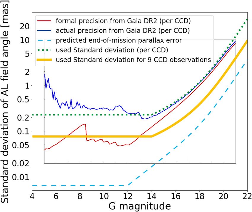
Fig. 8. Achievable standard error as a function of the input mass for
15 events. The two red events with a wide range for the input mass are
white dwarfs, where the mass can only be poorly determined from the
G magnitude. The uncertainty is roughly constant as a function of the
input mass. The diagonal lines indicate relative uncertainties of 15%,
30%, 50%, and 100%, respectively.
observations using other telescopes, and to combine the data.
Naively, one might expect that about 50% of the events should be
after this date (assuming a constant event rate each year). How-
ever, the events with a closest approach close to the epochs used
for Gaia DR2 are more difficult to treat by the Gaia reduction
(e.g. fewer observations due to blending). Therefore many back-
ground sources are not included in Gaia DR2. For 17 of these
future events, the achievable relative uncertainty is between 30
and 50%. Hence a combination with further precise measure-
Fig. 7. Distribution of the G magnitude of the source (top) and impact ments around the closest approach is needed to determine a pre-
parameter (bottom) as well as the resulting relative standard error of cise mass of the lens. To investigate the possible benefits of addi-
the mass determination for the investigated events. The grey, red, yel- tional observations, we repeated the simulation while adding two
low, and green parts correspond to a relative standard error better than 2D observations (each consists of two perpendicular 1D obser-
100%, 50%, 30%, and 15%, respectively. The thick black line shows the vations) around the epoch of the closest approach. We only con-
distribution of the input sample, where the numbers at the top show the
number of events in the corresponding bins. The thin black line in the
sidered epochs where the separation between the source and lens
bottom panel shows the events during the nominal mission. We note the stars is larger than 150 mas. Furthermore, we assumed that these
different bin width of 0.3300 below φmin = 200 and 100 above φmin = 200 in observations have the same precision as the Gaia observations.
the bottom panel. These results are listed in column σMobs /Min of Table A.2.
By including these external observations the results can be
improved by typically 2 to 5 percentage points. In extreme cases,
Figure 8 shows the achievable precision as a function of the input the results can even be improved by a factor of two when the
mass for a representative subsample. When the proper motion impact parameter is below 0.500 , since Gaia will lose measure-
of the background star is known from Gaia DR2, the uncer- ments due to combined readout windows. Events #63 to #65 are
tainty of the achievable precision is about 6%, and it is about special cases, since they are outside the extended mission, and
10% when the proper motion is unknown. We found that the Gaia only observes the leading tail of the event.
reachable uncertainty (in solar masses) depends only weakly on
the input mass, and is more connected to the impact parameter,
which is a function of all astrometric input parameters. Hence, 5.2. Multiple background sources
the scatter of the achievable precision is smaller when the proper
motion and parallax of the background source is known from For the 22 events of Klüter et al. (2018b) with multiple back-
Gaia DR2. For the 65 events with a relative standard error better ground sources, we tested three different cases. In the first, we
than 50%, Tables A.1 and A.2 list the achievable relative uncer- used all potential background sources. In the second, we only
used background sources where Gaia DR2 provides all five
tainty for each individual star as well as the determined scat-
astrometric parameters, and finally, we selected only those back-
ter for the extended mission σM10 . Table A.1 contains all events
ground sources for which the expected precision of Gaia indi-
during the nominal mission (before 2019.5), and also includes
vidual measurements is better than 0.5 mas. The expected rel-
the determined scatter using only the data of the nominal mission
ative uncertainties of the mass determinations for the different
σM5 . Table A.2 lists all future events with a closest approach
after 2019.5. cases are shown in Figs. 9 and A.1, as well as the expected rel-
ative uncertainties for the best case using only one background
Future events. In our sample, 383 events have a clos- source. By using multiple background sources, a better preci-
est approach after 2019.5 (Fig. 6 middle panel). These events sion of the mass determination can be reached. We note that
are of special interest, since it is possible to obtain further averaging the results of the individual fitted masses does not
A83, page 8 of 14J. Klüter et al.: Expectations on mass determination using astrometric microlensing by Gaia
Since we did not include the potential data points of the two
events predicted by Sahu et al. (2014), it might be possible to
reach an even higher precision. For those two events, Zurlo et al.
(2018) measured the deflection using the Very Large Telescope
equipped with the SPHERE10 . instrument. They derived a mass
of M = 0.150+0.062
−0.051 M . Comparing our expectations with their
mass determination, we expect to reach an error that is six times
smaller11 .
A further source that passes multiple background sources
is the white dwarf LAWD 37, for which we assume a mass of
0.65 M . Its most promising event, which was first predicted by
McGill et al. (2018), is in November 2019. McGill et al. (2018)
also mention that Gaia might be able to determine the mass with
an accuracy of 3%, however this was done without knowing the
scanning law for the extended mission. We expect an uncer-
tainty for the mass determination by Gaia of 0.12 M , which
corresponds to 19%. Within the extended Gaia mission the star
passes 12 further background sources. By combining the infor-
mation for all astrometric microlensing events by LAWD 37, this
result can be improved slightly (see Fig. 9 bottom panel). We
then expect a precision of 0.10 M (16%).
For 8 of the 22 lenses with multiple events, the expected stan-
dard error is better than 50%. The results of these events are
given in Table A.3. For a further three events the expected preci-
sion is between 50% and 100% (Figs. A.1g–A.1i). In addition to
our three cases, a more detailed selection of the used background
sources can be done, however, this is only meaningful once the
quality of the real data is known.
6. Summary and conclusion
In this work we showed that Gaia can determine stellar masses
for single stars using astrometric microlensing. For that purpose
we simulated the individual Gaia measurements for 501 pre-
dicted events during the Gaia era, using conservative cuts on the
resolution and precision of Gaia.
In a similar study, Rybicki et al. (2018) showed that Gaia
might be able to measure the astrometric deflection caused
by a stellar-mass black hole (M ≈ 10 M ), based on results
Fig. 9. Violin plot of the achievable uncertainties for the four differ- from a photometric microlensing event detected by OGLE
ent methods for Proxima Centauri (top) and LAWD 37 (bottom). For (Wyrzykowski et al. 2016). In addition, they claimed that for
each method the 16th, 50th, and 84th, percentile are shown. The shape faint background sources (G > 17.5 mag) Gaia might be able
shows the distribution of the 100 determined uncertainties caused by to detect the deflection of black holes more massive than 30 M .
varying the input parameter. This distribution is smoothed with a Gaus- In the present paper, however, we consider bright lenses, which
sian kernel. The green “violins” use all of the background sources. For are also observed by Gaia. Hence, due to the additional mea-
the blue violins only background sources with a five-parameter solution surements of the lens positions, we found that Gaia can measure
are used, and for the orange violins only stars with a precision in the
much smaller masses.
along-scan direction better than 0.5 mas and a five-parameter solution
are used. The red violins show the best results when only one source is In this study we did not consider orbital motion. However,
used. The dashed line indicates the median of this distribution. For each orbital motion can be included in the fitting routine for the anal-
method the number of used stars is listed below the violin. The miss- ysis of the real Gaia measurements. Gaia DR3 (expected for the
ing green violin of LAWD 37 is caused by no additional background end of 2021) will include orbital parameters for a fraction of the
stars with a two-parameter solution only. Hence it would be identical to contained stars. This information can be used to decide whether
the blue one (For the other events with multiple background stars see orbital motion should be considered or not.
Fig. A.1). We also assumed that source and lens can only be resolved if
both have individual readout windows. However, it might be pos-
sible to measure the separation in along-scan direction even from
necessarily increase the precision, since the values are highly the blended measurement in one readout window. Due to the
correlated. full width at half maximum of 103 mas (Fabricius et al. 2016)
Using all sources it is possible to determine the mass of Gaia might be able to resolve much closer lens-source pairs.
Proxima Centauri with a standard error of σ M = 0.012 M for
the extended ten-year mission of Gaia. This corresponds to a 10
Spectro-Polarimetric High-contrast Exoplanet REsearch
relative error of 10%, considering the assumed mass of M = 11
For an explanation of Violin plot see NIST: https:
0.117 M This is a factor of ∼0.7 better than the uncertainty of //www.itl.nist.gov/div898/software/dataplot/refman1/
the best event only (see Fig. 9 top panel, σ M = 0.019 M b
=16%). auxillar/violplot.htm.
A83, page 9 of 14A&A 640, A83 (2020)
The astrometric microlensing signal of such measurements is package for Astronomy (Astropy Collaboration 2013). This research made use
stronger. Hence, the results of events with impact parameters of matplotlib, a Python library for publication quality graphics (Hunter 2007).
smaller than the window size can be improved by a careful anal- This research made use of SciPy (Jones et al. 2001). This research made use of
NumPy (Van Der Walt et al. 2011).
ysis of the data. Efforts in this direction are foreseen by the Gaia
consortium for Gaia DR4 and DR5.
Via a Monte Carlo approach, we determined the expected References
precision of the mass determination and found that for 34 events
Astropy Collaboration (Robitaille, T. P., et al.) 2013, A&A, 558, A33
a precision better than 30%, and sometimes down to 5%, can Bond, I. A., Abe, F., Dodd, R. J., et al. 2001, MNRAS, 327, 868
be achieved. By varying the input parameters we found that our Bramich, D. M. 2018, A&A, 618, A44
results depend only weakly on selected input parameters. The Bramich, D. M., & Nielsen, M. B. 2018, Acta. Astron., 68, 183
scatter is of the order of 6% if the proper motion of the back- Branch, M. A., Coleman, T. F., & Li, Y. 1999, SIAM J. Sci. Comp., 21, 1
ground star is known from Gaia DR2 and of the order of 10% if Carrasco, J. M., Evans, D. W., Montegriffo, P., et al. 2016, A&A, 595, A7
Chung, S.-J., Zhu, W., Udalski, A., et al. 2017, ApJ, 838, 154
the proper motion is unknown. Furthermore, the dependency on Chwolson, O. 1924, Astron. Nachr., 221, 329
the selected input mass is even weaker. Dominik, M., & Sahu, K. C. 2000, ApJ, 534, 213
For 17 future events (closest approach after 2019.5), the Dong, S., Mérand, A., Delplancke-Ströbele, F., et al. 2019, ApJ, 871, 70
Gaia data alone are not sufficient to derive a precise mass. For Einstein, A. 1915, Sitzungsber. Preuss. Akad. Wiss., 47, 831
Einstein, A. 1936, Science, 84, 506
these events, it will be helpful to take further observations using, Fabricius, C., Bastian, U., Portell, J., et al. 2016, A&A, 595, A3
for example, the Hubble Space Telescope, the Very Large Tele- Gaia Collaboration (Prusti, T., et al.) 2016, A&A, 595, A1
scope, or the Very Large Telescope Interferometer. Such two- Gaia Collaboration (Brown, A. G. A., et al.) 2018, A&A, 616, A1
dimensional measurements can easily be included in our fitting Gould, A. 1992, ApJ, 392, 442
routine by adding two observations with perpendicular scanning Hog, E., Novikov, I. D., & Polnarev, A. G. 1995, A&A, 294, 287
Hunter, J. D. 2007, Comput. Sci. Eng., 9, 90
directions. We showed that two additional highly accurate mea- Jones, E., Oliphant, T., Peterson, P., et al. 2001, SciPy: Open source scientific
surements can improve the results significantly, especially when tools for Python
the impact parameter of the event is smaller than 100 . However, Klüter, J., Bastian, U., Demleitner, M., & Wambsganss, J. 2018a, A&A, 615,
since the results depend on the resolution and precision of the L11
Klüter, J., Bastian, U., Demleitner, M., & Wambsganss, J. 2018b, A&A, 620,
additional observations, these properties should be implemented A175
for such analyses, which is easily achievable. By doing so, our Lindegren, L., Hernández, J., Bombrun, A., et al. 2018, A&A, 616, A2
code can be a powerful tool to investigate different observation Luri, X., Brown, A. G. A., Sarro, L. M., et al. 2018, A&A, 616, A9
strategies. The combination of Gaia data and additional informa- McGill, P., Smith, L. C., Evans, N. W., Belokurov, V., & Smart, R. L. 2018,
tion might also lead to better mass constraints for the two pre- MNRAS, 478, L29
McGill, P., Smith, L. C., Evans, N. W., Belokurov, V., & Lucas, P. W. 2019,
viously observed astrometric microlensing events of Stein 51b MNRAS, 487, L7
(Sahu et al. 2017) and Proxima Centauri (Zurlo et al. 2018). For Miyamoto, M., & Yoshii, Y. 1995, AJ, 110, 1427
the latter, Gaia DR2 does not contain the background sources. Mustill, A. J., Davies, M. B., & Lindegren, L. 2018, A&A, 617, A135
However, we are confident that Gaia has observed both back- Nielsen, M. B., & Bramich, D. M. 2018, Acta. Astron., 68, 351
Paczyński, B. 1986, ApJ, 301, 503
ground stars. Finally, once the individual Gaia measurements Paczyński, B. 1991, ApJ, 371, L63
are published (DR4 or final data release), the code can be used Paczyński, B. 1995, Acta. Astron., 45, 345
to analyse the data, which will result in multiple well-measured Paczyński, B. 1996, ARA&A, 34, 419
masses of single stars. The code can also be used to fit the motion Pourbaix, D., Tokovinin, A. A., Batten, A. H., et al. 2004, A&A, 424, 727
of multiple background sources simultaneously. When combin- Proft, S., Demleitner, M., & Wambsganss, J. 2011, A&A, 536, A50
Rybicki, K. A., Wyrzykowski, Ł., Klencki, J., et al. 2018, MNRAS, 476, 2013
ing these data, Gaia can determine the mass of Proxima Centauri Sahu, K. C., Bond, H. E., Anderson, J., & Dominik, M. 2014, ApJ, 782, 89
with a precision of 0.012 M . Sahu, K. C., Anderson, J., Casertano, S., et al. 2017, Science, 356, 1046
Salim, S., & Gould, A. 2000, ApJ, 539, 241
Shvartzvald, Y., Yee, J. C., Skowron, J., et al. 2019, AJ, 157, 106
Acknowledgements. We gratefully thank the anonymous referee, whose sug- Torres, G., Andersen, J., & Giménez, A. 2010, A&ARv, 18, 67
gestions greatly improved the paper. This work has made use of results from Udalski, A. 2003, Acta. Astron., 53, 291
the ESA space mission Gaia, the data from which were processed by the Gaia Van Der Walt, S., Colbert, S. C., & Varoquaux, G. 2011, Comput. Sci. Eng., 13,
Data Processing and Analysis Consortium (DPAC). Funding for the DPAC 22
has been provided by national institutions, in particular the institutions par- Walker, M. A. 1995, ApJ, 453, 37
ticipating in the Gaia Multilateral Agreement. The Gaia mission website is: Wyrzykowski, Ł., Kostrzewa-Rutkowska, Z., Skowron, J., et al. 2016, MNRAS,
http://www.cosmos.esa.int/Gaia. Two (U. B., J. K.) of the authors are 458, 3012
members of the Gaia Data Processing and Analysis Consortium (DPAC). This Zang, W., Shvartzvald, Y., Wang, T., et al. 2020, ApJ, 891, 3
research has made use of the SIMBAD database, operated at CDS, Strasbourg, Zhu, W., Calchi Novati, S., Gould, A., et al. 2016, ApJ, 825, 60
France. This research made use of Astropy, a community-developed core Python Zurlo, A., Gratton, R., Mesa, D., et al. 2018, MNRAS, 480, 236
A83, page 10 of 14J. Klüter et al.: Expectations on mass determination using astrometric microlensing by Gaia
Appendix A: Additional material
Table A.1. Estimated uncertainties of mass measurements using astrometric microlensing with Gaia for single events that have an epoch of the
closest approach during the nominal Gaia mission.
# Name-lens DR2_ID-lens DR2_ID-source T CA Min σ M10 σ M10 /Min σ M5
Jyear M M M
1 HD 22399 488099359330834432 488099363630877824∗ 2013.711 1.3 ±0.60+0.07
−0.05
47%
2 HD 177758 4198685678421509376 4198685678400752128∗ 2013.812 1.1 ±0.41+0.04
−0.04 36%
3 L 820-19 5736464668224470400 5736464668223622784∗ 2014.419 0.28 ±0.058+0.004
−0.004 21% ±0.11+0.01
−0.01
4 2081388160068434048 2081388160059813120 ∗
2014.526 0.82 ±0.39+0.05
−0.04 47%
5 478978296199510912 478978296204261248 2014.692 0.65 ±0.24+0.02
−0.02 36% ±0.49+0.04
−0.04
6 G 123-61B 1543076475514008064 1543076471216523008∗ 2014.763 0.26 ±0.099+0.010
−0.009 37% +0.02
±0.18−0.02
7 L 601-78 5600272625752039296 5600272629670698880 ∗
2014.783 0.21 ±0.041+0.003
−0.004 19% ±0.068+0.006
−0.005
8 UCAC3 27-74415 6368299918479525632 6368299918477801728∗ 2015.284 0.36 ±0.047+0.005
−0.005
13% +0.01
±0.11−0.01
9 BD+00 5017 2646280705713202816 2646280710008284416∗ 2015.471 0.58 ±0.18+0.02
−0.02 30% ±0.44+0.04
−0.05
10 G 123-61A 1543076475509704192 1543076471216523008∗ 2016.311 0.32 ±0.079+0.007
−0.008 24% +0.02
±0.14−0.02
11 EC 19249-7343 6415630939116638464 6415630939119055872∗ 2016.650 0.26 ±0.099+0.008
−0.008 38%
12 5312099874809857024 5312099870497937152 2016.731 0.07 ±0.0088+0.0006
−0.0006
12% ±0.0098+0.0010
−0.0007
13 PM J08503-5848 5302618648583292800 5302618648591015808 2017.204 0.65 ±0.17+0.02
−0.02 26% ±0.29+0.03
−0.03
14 5334619419176460928 5334619414818244992 2017.258 0.65 ±0.23+0.02
−0.02 35% ±0.43+0.04
−0.03
15 Proxima Cen 5853498713160606720 5853498708818460032 2017.392 0.12 ±0.034+0.003
−0.003 29% ±0.082+0.006
−0.006
16 Innes’ star 5339892367683264384 5339892367683265408 2017.693 0.33 ±0.16+0.02
−0.01 48% ±0.22+0.02
−0.02
17 L 51-47 4687511776265158400 4687511780573305984 2018.069 0.28 ±0.035+0.003
−0.003 12% ±0.046+0.004
−0.004
18 4970215770740383616 4970215770743066240 2018.098 0.65 ±0.076+0.008
−0.005
12% +0.02
±0.21−0.02
19 BD-06 855 3202470247468181632 3202470247468181760∗ 2018.106 0.8 ±0.38+0.05
−0.05
46% ±0.72+0.19
−0.08
20 G 217-32 429297924157113856 429297859741477888∗ 2018.134 0.23 ±0.018+0.002
−0.002 7.5% ±0.040+0.003
−0.004
21 5865259639247544448 5865259639247544064∗ 2018.142 0.8 ±0.053+0.008
−0.006
6.6% +0.02
±0.12−0.02
22 HD 146868 1625058605098521600 1625058605097111168∗ 2018.183 0.92 ±0.060+0.005
−0.005
6.5% ±0.14+0.02
−0.02
23 Ross 733 4516199240734836608 4516199313402714368 2018.282 0.43 ±0.067+0.005
−0.006
15% ±0.13+0.01
−0.02
24 LP 859-51 6213824650812054528 6213824650808938880∗ 2018.359 0.43 ±0.19+0.03
−0.03 43%
25 L 230-188 4780100658292046592 4780100653995447552 2018.450 0.15 ±0.073+0.007
−0.004 49% +0.01
±0.11−0.01
26 HD 149192 5930568598406530048 5930568568425533440∗ 2018.718 0.67 ±0.043+0.007
−0.004 6.3% ±0.12+0.01
−0.01
27 HD 85228 5309386791195469824 5309386795502307968∗ 2018.751 0.82 ±0.043+0.004
−0.004 5.1% ±0.65+0.05
−0.06
28 HD 155918 5801950515627094400 5801950515623081728∗ 2018.773 1 ±0.13+0.02
−0.02 13% ±0.35+0.03
−0.03
29 HD 77006 1015799283499485440 1015799283498355584∗ 2018.796 1 ±0.42+0.05
−0.05
41%
30 Proxima Cen 5853498713160606720 5853498713181091840 2018.819 0.12 ±0.020+0.002
−0.002 16% ±0.052+0.005
−0.005
31 HD 2404 2315857227976341504 2315857227975556736 ∗
2019.045 0.84 ±0.19+0.02
−0.02 22%
32 LP 350-66 2790883634570755968 2790883634570196608∗ 2019.299 0.32 ±0.15+0.02
−0.02 46%
33 HD 110833 1568219729458240128 1568219729456499584∗ 2019.360 0.78 ±0.056+0.005
−0.004 7.2%
Notes. The table lists the name (Name-Lens) and Gaia DR2 source ID (DR2_ID-Lens) of the lens and the source ID of the background sources
(DR2_ID-source). An asterisk indicates that Gaia DR2 only provides the position of the sources. In addition, the table lists the epoch of the closest
approach (T CA ) and the assumed mass of the lens (Min ). The expected precision arising from the use of data from the extended ten-year mission
is given in (σ M10 ), including the uncertainty due to the errors in the input parameters, and as a percentage (σ M10 /Min ). The expected precision
arising from the use of data from the nominal five-year mission is given in (σ M5 ) if it is below 100% of the input mass.
A83, page 11 of 14You can also read