Molinaro, L., Lawson, D. J., Pagani, L., & et al. (2021). A Chromosome-Painting Based Pipeline to Infer Local Ancestry under Limited Source ...
←
→
Page content transcription
If your browser does not render page correctly, please read the page content below
Molinaro, L., Lawson, D. J., Pagani, L., & et al. (2021). A
Chromosome-Painting Based Pipeline to Infer Local Ancestry under
Limited Source Availability. Genome Biology and Evolution, 13(4),
[evab025]. https://doi.org/10.1093/gbe/evab025

Peer reviewed version
License (if available):
CC BY
Link to published version (if available):
10.1093/gbe/evab025

Link to publication record in Explore Bristol Research
PDF-document

This is the author accepted manuscript (AAM). It first appeared online via Oxford University Press at
https://doi.org/10.1093/gbe/evab025. Please refer to any applicable terms of use of the publisher.

University of Bristol - Explore Bristol Research
General rights

This document is made available in accordance with publisher policies. Please cite only the
published version using the reference above. Full terms of use are available:
http://www.bristol.ac.uk/red/research-policy/pure/user-guides/ebr-terms/
A chromosome-painting based pipeline to infer local ancestry under
limited source availability

Ludovica Molinaro1,2, Davide Marnetto1, Mayukh Mondal1, Linda Ongaro1,2, Burak Yelmen1,2,
Daniel John Lawson3, Francesco Montinaro1,4*, Luca Pagani1,5*

1 Estonian Biocentre, Institute of Genomics, University of Tartu, Tartu, 51010, Estonia
2 Institute of Molecular and Cell Biology, University of Tartu, Tartu, 51010, Estonia
3 Medical Research Council Integrative Epidemiology Unit, Department of Population Health

                                                                                                                                Downloaded from https://academic.oup.com/gbe/advance-article/doi/10.1093/gbe/evab025/6135079 by guest on 16 March 2021
Sciences, Bristol Medical School, University of Bristol, Bristol, BS8 2BN, UK
4 Department of Biology-Genetics, University of Bari, Bari, 70126, Italy
5 Department of Biology, University of Padova, Padova, 35121, Italy

*these senior authors contributed equally to the work

Corresponding author: Ludovica Molinaro: lu.molinaro8@gmail.com

Abstract

Contemporary individuals are the combination of genetic fragments inherited from ancestors
belonging to multiple populations, as the result of migration and admixture. Isolating and
characterising these layers is crucial to the understanding of the genetic history of a given
population. Ancestry deconvolution approaches make use of a large amount of source
individuals, therefore constraining the performance of local ancestry inferences when only few
genomes are available from a given population. Here we present WINC, a local ancestry
framework derived from the combination of ChromoPainter and NNLS approaches, as a
method to retrieve local genetic assignments when only a few reference individuals are
available. The framework is aided by a score assignment based on source differentiation to
maximise the amount of sequences retrieved, and is capable of retrieving accurate ancestry
assignments when only two individuals for source populations are used.

Keywords

Admixture, Local Ancestry, ChromoPainter, NNLS

Significance Statement

As the results of migration and admixture between populations, contemporary genomes can
be seen as a mosaic, where each piece is an inherited genomic fragment. Isolating and
characterising these fragments helps the understanding of the genetic and evolutionary history
of a given population. The key approach to study the admixed fragments is Ancestry
Deconvolution, though it is generally limited by both the quality and amount of the genomes
of source populations. Here we developed a local ancestry framework derived from the

 © The Author(s) 2021. Published by Oxford University Press on behalf of the Society for Molecular Biology and Evolution.
 This is an Open Access article distributed under the terms of the Creative Commons Attribution Non-Commercial License
 (http://creativecommons.org/licenses/by-nc/4.0/), which permits non-commercial re-use, distribution, and reproduction in any
 medium, provided the original work is properly cited. For commercial re-use, please contact journals.permissions@oup.com

                                       http://mc.manuscriptcentral.com/gbe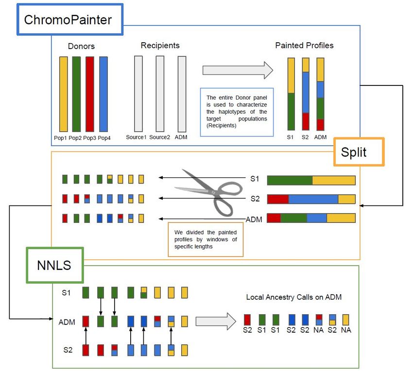
combination of ChromoPainter and NNLS approaches, as a method to perform Ancestry
Deconvolution when only a few reference individuals are available.

                                                                                    Downloaded from https://academic.oup.com/gbe/advance-article/doi/10.1093/gbe/evab025/6135079 by guest on 16 March 2021

                          http://mc.manuscriptcentral.com/gbe
Introduction
In the last decade, the advent of dense genotyping arrays and high throughput sequencing
technologies has paved the way to the development of methods aimed at reconstructing Local
Ancestry patterns along the chromosomes.
A large variety of local ancestry deconvolution methods have been proposed, harnessing
Downloaded from https://academic.oup.com/gbe/advance-article/doi/10.1093/gbe/evab025/6135079 by guest on 16 March 2021
different statistical algorithms such as Hidden Markov Models (HMM) (HapMix (Price et al.,
2009), LAMP-LD (Baran et al., 2012), ELAI (Guan, 2014), MOSAIC (Salter-Townshend and
Myers, 2019)), Principal Component analysis (PCAdmix (Brisbin et al., 2012)) and machine
learning classification tools (RF-Mix (Maples et al., 2013)).
Most Local Ancestry Inference (LAI) methods available to date, identify fragments putatively
descending from a limited number of reference populations, for which tens of individuals are
typically required. Although a reasonable amount of data for most of the contemporary human
groups are available (Yelmen et al., 2019), this is not the case for many key populations. Some
human groups remain poorly sampled (hindered by social, geographic or ethical factors), and
historical populations are often incompletely captured by ancient DNA, which is reliant on
preservation conditions, burial practice, extent of archaeological activity and other biasing
factors. Furthermore and beyond the human realm, for contemporary or extinct species, few
individuals are usually available to represent source populations due to the limited availability
of samples or resources. A limited number of source individuals causes an under-estimation
of the genetic diversity within populations, increasing the assignment error of the traditional
LAI methods.
In this study, we propose that leveraging a larger panel of populations to genetically
characterize both the sources and the admixed population could yield a better performance
even when little amounts of source individuals are available for the analyses.
ChromoPainter provides the best approach to overcome the issue of lack of data for the
sources of the target admixed population, as it uses the genetic information acquired from a
large panel of populations, even unrelated to the admixture event, to describe (or paint) both
sources and target individuals. A NNLS (Non-Negative Least Squares) is then used to
summarize the painting information.
ChromoPainter/NNLS (Hellenthal et al., 2014; Lawson et al., 2012; Leslie et al., 2015)
approach has been successfully employed to reconstruct the global ancestry of modern-day
http://mc.manuscriptcentral.com/gbeand ancient populations, and simulation-based comparisons showed that it yields high
accuracy at a genome wide level, even when a limited number of reference samples are
available (Busby et al., 2016; Hofmanová et al., 2016; Järve et al., 2019; Montinaro et al.,
2015; Ongaro et al., 2019; van Dorp et al., 2015).
We propose to turn the ChromoPainter/NNLS framework into a Local Ancestry Inference tool,
by applying the NNLS step on genetic windows, instead of the entire genomes. This approach
Downloaded from https://academic.oup.com/gbe/advance-article/doi/10.1093/gbe/evab025/6135079 by guest on 16 March 2021
could leverage on a large number of donor populations to characterize not only the admixed
targets, but also the source populations, and thus provide a versatile solution when only a few
samples are available for source populations.
We tested the performance of the proposed approach through coalescent simulations,
validated it on an additional set of simulated individuals and applied it to real case scenarios.
All simulated individuals were admixed 100 generations ago, a limit date for which most dating
tools can detect an admixture event (Moorjani et al., 2011).
We benchmarked our performance against three Local Ancestry tools: a machine learning
based tool (RFmix, a commonly used LAI software), a Principal Component analysis based
tool (PCAdmix) and a HMM based tool (ELAI, shown to outperform many of the state-of-the-
art methods (Geza et al., 2018) and to perform well even in regions with small ancestral track
length (Guan, 2014)).
The results showed that our method is capable of outcompeting all methods and particularly
ELAI, which shows higher performances than PCAdmix and RFmix, when harnessing admixed
individuals whose sources diverged at least 30 kiloyears ago (kya), using as little as two
individuals as sources.
RESULTS
Proposed window-based ChromoPainter/NNLS framework
As the core of our strategy we used the recently developed approach implemented in the
ChromoPainter/NNLS (Hellenthal et al., 2014; Lawson et al., 2012; Leslie et al., 2015)
algorithm (the combination of ChromoPainter and NNLS algorithms).
In a given phased dataset, ChromoPainter (Lawson et al., 2012) identifies the closest
neighbour “donor” for any “recipient” individual haplotype. Along the chromosome, the
combination of all the identified closest neighbours summarises the different ancestry of an
http://mc.manuscriptcentral.com/gbeindividual. Given the high complexity and computational resources needed for computing the
whole set of genealogies, ChromoPainter exploits the approximation provided in the Hidden
Markov Model developed by Li and Stephens (2003) (Li and Stephens, 2003), reconstructing
recipient individuals as a combination of genomic segments, or chunks, “donated” by any other
individual in the dataset. The information is then stored in a copying vector, an array that
summarizes the amount of genome copied by a given recipient from each donor sample.
However, the coalescent events in natural groups may predate the time of population split,
Downloaded from https://academic.oup.com/gbe/advance-article/doi/10.1093/gbe/evab025/6135079 by guest on 16 March 2021
therefore creating only small differences in the amount of genetic fragments copied by closely
related populations, adding a confounding factor in the ancestral deconvolution approach. This
limitation is solved using a multiple linear regression approach, in which a modification of the
Non-Negative Least Square approach (NNLS) is exploited to reconstruct the painting profile
of a given individual as a combination of copying vectors from a set of source individuals or
populations. In this approach, the target admixed individuals are usually set as recipients, and
the putative sources of the admixture as donors. We propose to set as recipients both the
admixed individuals and the unadmixed sources, in order to paint them with a large panel of
donor populations not necessarily related with the admixture event.
Here we develop a framework for performing Local Ancestry Decolvolution using
ChromoPainter/NNLS onto genomic windows that approximate the expected ancestry tiling in
an admixed individual, and named it WINC as short for Window-based NNLS/ChromoPainter.
Unlike the regular pipeline, we applied it on 500 kilo-base (kb) genomic windows, rather than
the whole genomes. The length of 500kb genomic windows has been chosen to fall within the
expected chunk length of an admixture event that happened 100 generations ago (see
methods). In doing so, we aim to convey ChromoPainter/NNLS accuracy as a global ancestry
estimator onto a genomic localized context, hence turning it into a local ancestry tool.
A schematic representation of the process is shown in Figure 1. More in detail i) we performed
a ChromoPainter run in which source and target individuals are painted using the entire donor
panel. The donor panel is composed of presumably unadmixed groups. The admixed target
populations were set as recipients, along with the source populations. Setting as recipients
both the target and the source individuals allowed us to obtain the copying vectors for both,
which were then used for the following step. ii) For each painted haplotype, we splitted the
copying vector into genomic windows of the same length. For any window, we averaged the
amount of genome copied from any donor populations and normalized the resulting copying
vector to sum 1. iii) We then moved to the NNLS step, in which we described each target
individual as a mixture of the selected source populations. The NNLS approach identifies the
sources’ copying vector that better match the copying vector of recipient populations as
estimated by ChromoPainter. In this way, for each window belonging to admixed individuals,
http://mc.manuscriptcentral.com/gbewe used NNLS to assign the window to one of the putative sources. The assignment indicates
the proportion of the admixed copying vector that matches each source’s copying vector. iv)
Each ancestry assignment proportion can be seen as a score (Assignment Score or AS), on
which we apply several cutoffs. We then averaged the window-based copying vectors through
all the individuals.
We tested the performance of the proposed approach through coalescent simulations,
Downloaded from https://academic.oup.com/gbe/advance-article/doi/10.1093/gbe/evab025/6135079 by guest on 16 March 2021
validated it on an additional simulated dataset and finally on real individuals, and benchmarked
our performance against other LAI tools. Each analysis was performed twice, first using 50
individuals as sources and then only 2 (100 and 4 haplotypes respectively), but maintaining in
both cases a large number of donor populations unrelated to the admixture event.
FIGURE 1 - Schematic representation of WINC approach. WINC is based on the
ChromoPainter/NNLS framework, with the additional step of splitting the copying vectors
resulting from the ChromoPainter (CP) run before analyzing them through the NNLS step.
First step: ChromoPainter run. CP identifies the closest neighbour “donor” for any “recipient”
individual haplotype. ChromoPainter then reconstructs the recipient individuals as a
combination of genomic segments, or chunks, “donated” by any other individual in the dataset.
The information is then stored in copying vectors, where, for each recipient haplotype, it is
http://mc.manuscriptcentral.com/gbeindicated which donor individual is the closest neighbour. In this way, we obtain the copying
vectors of our target populations: both the sources and the admixed individuals. Second step:
splitting copying vectors. We then split the copying vectors in genomic windows of the same
length. Window size depends on the ancestry chunks, which in turn depends on the amount
of generations since the admixture. Third step: performing Non-Negative Least Square
(NNLS) analyses on the copying vector's genomic windows obtained from the previous step.
The NNLS step assigns a window to a specific ancestry, by reconstructing the painting profile
Downloaded from https://academic.oup.com/gbe/advance-article/doi/10.1093/gbe/evab025/6135079 by guest on 16 March 2021
of a given individual as a combination (or proportion) of copying vectors from the source
individuals.
Evaluation Parameters
All Local Ancestry Inference (LAI) tools tested here assign a probability of ancestry to each
genomic window. On the other hand, our approach employs the proportion assignment given
by the NNLS (see methods). In both cases, we refer to the value assignments as Assignment
Score (AS). The AS values range from 0 to 1 and they are used to evaluate the performance
of all tools by applying several cutoffs.
We set different thresholds for each run in order to remove windows with an AS (or ancestry
assignment probability/proportion) lower than the threshold. All removed windows are then
labeled as "Unassigned". We set for all LAI tools the following AS thresholds: .55, .6, .65, .7,
.75, .8, .85, .9, .91, .92, .93, .94, .95, .96, .97, .98, 99.
Given the presence of unassigned values, we accounted for accuracy and assignation
separately. We set Accuracyg as the portion of windows correctly assigned given all genome
windows, taking into consideration both the assigned and the unassigned windows. We set
Accuracya as the portion of windows correctly assigned given only the windows that passed
the threshold, therefore not taking into account the ‘Unassigned’ blocks. We calculated
separately ‘Assigned Genome’ as the portion of all the windows that reached the AS threshold.
Simulating Admixed Individuals
We simulated a Test Set of 13 populations with different population sizes and with divergence
times ranging from 250 to 4000 generations (7.5 kilo year ago (kya) to 120 kya), to represent
current European, East Asian and African groups, following a modified Van Dorp et al model
(van Dorp et al., 2015).
We then added seven sister groups, characterised by a divergence time from their sister group
http://mc.manuscriptcentral.com/gbeof 100 generations (3 kya), for a total of 20 simulated populations. These additional sister
groups were not present in the model of Van Dorp et al, and were labelled as “Ghost” (GST)
(Figure S1). These populations were later used to create admixed groups, but were not
included in any following step, as in a real scenario it would not be possible to perform Ancestry
Deconvolution with the actual sources of the admixture.
We generate eight two-ways admixed populations combining pairs of simulated Ghost demes,
and one three-ways admixed population with admix-simu
Downloaded from https://academic.oup.com/gbe/advance-article/doi/10.1093/gbe/evab025/6135079 by guest on 16 March 2021
(https://github.com/williamslab/admix-simu) with an admixture time of 100 generations and
proportions of 70%-30% and 40%-30%-30% respectively (See in Supplementary Table S1).
Similarly, we also simulated an Empirical Set of three two-ways admixed populations and one
three-ways admixed population from the 1000 Genome project (The 1000 Genomes Project
Consortium, 2015) using admixture proportions and generation times as per the Test Set
(70%-30% for the two ways, 40%-30%-30% for the three ways and 100 generations since the
admixture in all cases). We simulated the admixture events between a European (TSI, Toscani
in Italy) and African (YRI, Yoruba in Nigeria) population, European (TSI) and Asian (CHB, Han
Chinese in Beijing) population, within European populations (TSI and FIN, Finnish in Finland).
The three-way continental admixture was created between YRI, CHB and TSI. We used CEU
(Utah residents with European ancestry) as a source population to retrieve TSI fragments,
ESN (Esan in Nigeria) for YRI and CHS (Han Chinese South) for CHB. To retrieve FIN
fragments, we set as source all FIN individuals not used to create the admixed population TSI-
FIN. As donor panel, we used all populations from the 1000 Genomes Project.
Global ancestry estimates
First, we analyzed the pairwise genetic distance among all pairs of simulated populations from
the Test Set and showed that they are consistent with those observed among modern
populations (Figure S2 and S3). We then applied ChromoPainter/NNLS global ancestry
methodology on the entire chromosome and showed that it correctly assigns the two
ancestries (Figure S4), with a discrepancy of 0.01% when the sources diverged 75 kya and
10% when they diverged just 7.5 kya.
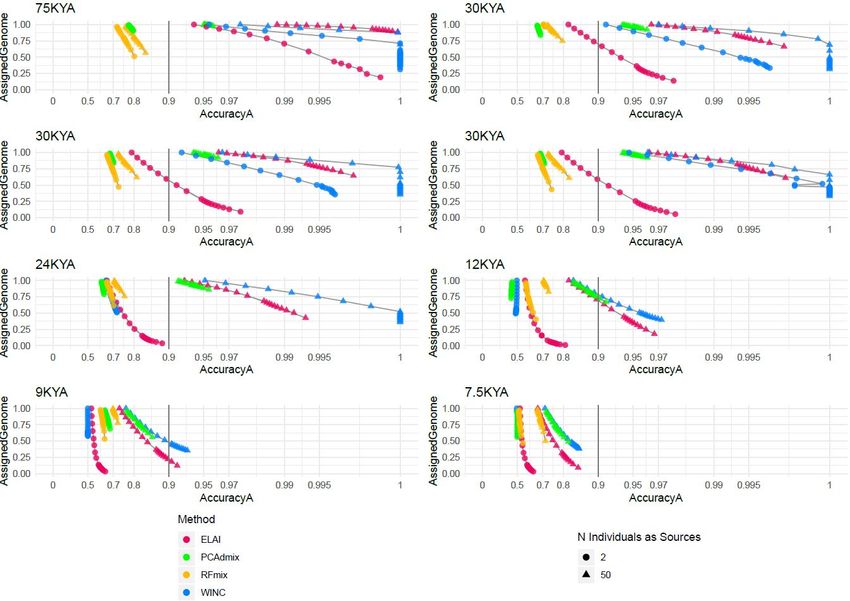
WINC performance on the Testing Set
To test our approach, we applied WINC on a set of simulated individuals (Test Set). All
populations are characterized by a distant admixture time (100 generation), which causes the
ancestral fragments to be relatively small in all target individuals. On the other hand all
http://mc.manuscriptcentral.com/gbeadmixed populations vary on the similarity of the sources of the admixture, given by the
different divergence time between sources. Thus, we expect that the LAI tools more robust in
inferring ancestries in small regions will yield high performances. On the other hand, we expect
that each tool performance will decrease as the divergence between sources decreases,
despite the admixture generations. We compared WINC with RFmix, PCAdmix and ELAI. To
compare LAI tools we considered both Assigned Genome, the portion of the windows that
reached the threshold, and accuracya, an accuracy computed only on windows for which
Downloaded from https://academic.oup.com/gbe/advance-article/doi/10.1093/gbe/evab025/6135079 by guest on 16 March 2021
ancestry assignment was performed.
Overall, RFmix performance does not exceed the accuracya of 85% in any target population
(Figure 2), probably due to the high number of generation elapsed since the admixture (Dias-
Alves et al., 2018) (Figure S5). This is shown when using 50 individuals per source as well as
2. WINC outcompetes RFMix, showing that our framework could detect ancestries in a target
population with small ancestry tiles.
PCAdmix results are comparable with WINC and ELAI when using 50 individuals per source.
When 2 individuals are employed to deconvolute the target population, PCAdmix accuracya is
always lower than 0.8, regardless of the divergence between sources (Figure 2).
Of all tested tools, the only one matching WINC’s performance appears to be ELAI (Figure 2).
In fact, when using 50 samples for each source population, both ELAI and WINC display a
comparable amount of Assigned Genome and accuracy levels for all divergences between
the sources (Figure 2 and Table S2-S7).
Supported by the promising evidence, we moved to test our approach using only two
individuals per source, the main focus of our investigation.
ELAI and WINC show comparable levels of accuracya and Assigned Genome when only two
individuals are used per source. For populations with highly differentiated sources and older
split times, such as 75 kya or 30 kya, WINC assigns up to 99% of the genome with a minimum
accuracya of 0.9 (Figure 2, Table S2-S7). When tested on the 30 kya populations, WINC
outperforms ELAI in terms of accuracy levels reached and proportion of Assigned Genome
maintained. For more recent split times (up to 24 kya), both WINC and ELAI show a decrease
in accuracya and amount of genome retrieved, as expected when the sources of the admixture
are genetically similar.
We further provide specific results for both WINC and ELAI considering only one AS threshold
(0.8), to provide performance for a standard run under default parameters (Figures S6-S9).
http://mc.manuscriptcentral.com/gbeGiven that RFmix is suited for more recent admixture times (Figure S5) and PCAdmix does
not reach high performance levels when only two individuals are used as sources, we
performed the subsequent tests using only ELAI as a benchmark.
Downloaded from https://academic.oup.com/gbe/advance-article/doi/10.1093/gbe/evab025/6135079 by guest on 16 March 2021
FIGURE 2 - WINC performances on the Test Set compared to several Local Ancestry tools:
ELAI, PCAdmix and RFmix. The eight panels represent results for different admixed
populations with different divergence times. Within each series, different data points linked by
a grey line represent experiments run using increasingly stringent AS thresholds, and for which
a non zero amount of genomes was assigned to at least one ancestry by that particular LAI
method. X-axis shows accuracy(a) values, y-axis shows the proportion of genome windows
retrieved. Red points indicate the results obtained using ELAI, green dots indicate PCAdmix
results, orange dots list RFmix results, while blue points list WINC results. Triangles indicate
Local Ancestry results using 50 individuals per source, while dots list results using 2
individuals. We note that in the ‘12 KYA’ panel, when two individuals are used as reference, both
PCAdmix and WINC accuracy values decrease with increasingly stringent AS thresholds. This
effect is however minor (PCAdmix accuracy values range from 0.44 to 0.43 and WINC values
range from 0.51 to 0.49).
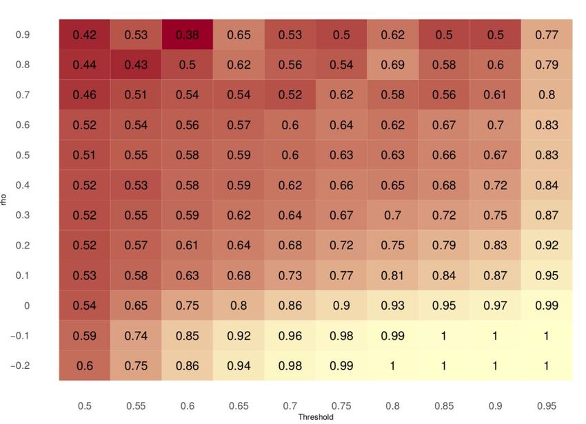
http://mc.manuscriptcentral.com/gbeWINC calibration using a Correlation-Assignment Score (C-AS) matrix
LAI approaches are expected to have a higher accuracy when the admixing sources are
genetically distant at the locus of interest. The more two sources are differentiated at a given
genomic window, the easier it should be for NNLS to assign a haplotype to one or the other
source population. We can leverage the similarity between sources to predict when NNLS has
Downloaded from https://academic.oup.com/gbe/advance-article/doi/10.1093/gbe/evab025/6135079 by guest on 16 March 2021
sufficient information to correctly infer the local ancestries, providing a calibration for WINC.
To assess the similarity between different sources, we computed a Pearson correlation
coefficient (rho) between ChromoPainter copying vectors obtained on the same window for
each pair of source populations. We then performed the NNLS analysis applying different
cutoffs, therefore removing all windows where the AS was lower than the specified threshold.
We calculated the accuracy obtained considering windows in ten equally spaced rho values
and AS thresholds. In doing so, we obtained a Correlation-Assignment Score (C-AS) matrix
(Figure 3) that, given different values of similarity between sources (correlation) and
assignment score (AS), should inform on the expected accuracy values.
FIGURE 3. Reference C-AS matrix on Test Set, a correlation matrix obtained using rho values
http://mc.manuscriptcentral.com/gbebetween sources and Assignment Scores. Each slot indicates accuracya values obtained by
selecting a given set of Assignment Scores (x axis) threshold and rho values of similarity
between source populations (y-axis). High accuracya values are listed with lighter colours, low
accuracya values are indicated by darker colours.
Application of Reference C-AS matrix and effects on WINC performance
Downloaded from https://academic.oup.com/gbe/advance-article/doi/10.1093/gbe/evab025/6135079 by guest on 16 March 2021
We tested the applicability of the C-AS matrix (estimated on the Test Set) on the Empirical Set
(see Figure 3 and Figure S10 for a schematic representation). For a given correlation in a
specific window, we used the minimum AS threshold needed to obtain the desired accuracya
value. We analyzed the overall performance and transferability of the C-AS matrix on the
Empirical Set and compared it with the results obtained by selecting the windows only by AS
thresholds.
Our tool operates with high accuracya values (over 0.9) also on the Empirical Set when 50
individuals are available for the Local Ancestry Inferences, and the sources are genetically
differentiated (See Figure 4 panel A and B and Tables S8-S9). In fact, similarly with the Test
Set results on populations with genetically similar sources, all LAI tools tested do not reach
satisfactory accuracya levels on TSI-FIN (Figure 4 Panel C and Table S10).
We thus moved to study its performances when only two individuals per source were set. We
observed that, for both TSI-YRI and TSI-CHB populations, WINC calibrated with the C-AS
matrix performs equally well to WINC alone in terms of accuracya, but retrieves higher portions
of the genome (Figure 4 panel A and B and Tables S8-S9), with the additional notable
difference that WINC+C-AS is predictable in its outcome. By applying the C-AS matrix to WINC
we could in fact assign windows with the desired accuracya, with the only exception being
reaching an observed accuracya of ~0.97 when the expected one was set at 0.99 (See Figure
S11 and S12 and Table S8-S9).
Differently from WINC alone, WINC + C-AS matrix tends to not assign any genomic window
of TSI-FIN (maximum 0.1%), when threshold values were set to 0.85 or higher (Figure 4 panel
C and Table S10), hence providing an effective way of drastically reducing false positives
when true positives cannot be obtained at all.
The C-AS matrix, created from the Test Set and applied to the Empirical Set, returned windows
that reached the selected desired accuracya, showing its efficacy when used on a different
dataset. We also applied the C-AS matrix on the Test set, as a control (Figure S13).
http://mc.manuscriptcentral.com/gbeAdditionally we investigated WINC performance of different window lengths: 1000 kb, 100 kbs
and on variable lengths depending on the SNP-density (See Supplementary Figure S14-S15)
and confirmed 500kb to be the optimal window size for the current study.
Downloaded from https://academic.oup.com/gbe/advance-article/doi/10.1093/gbe/evab025/6135079 by guest on 16 March 2021
FIGURE 4 - WINC and WINC+C-AS performances compared with ELAI on the Empirical Set.
Red points indicate the results obtained using ELAI, blue points list WINC results and light
blue points list WINC+C-AS performances. Triangles indicate Local Ancestry results using 45
individuals per source, while dots lists results using 2 individuals. On the x-axis we listed
accuracya values, computed only on windows for which ancestry assignment was performed,
and on the y-axis we listed the proportion of genome windows retrieved.
Evaluating WINC performance on three-way admixtures
As a proof of principle, we show the analyses on the three ways admixtures simulated in the
Test Set and Empirical Set jointly. Results on the Test Set show that ELAI outcompetes both
WINC and WINC+C-AS when harnessing the ancestries of a three-ways admixture, even
when only a few individuals are used as source. On the other hand, on the Empirical Set,
WINC and WINC+C-AS outperformed ELAI when two individuals are set per source (See
http://mc.manuscriptcentral.com/gbeFigure S16 and S17 and Table S11-S12).
Evaluating WINC performance on real data
Lastly, we applied the WINC and WINC+C-AS matrix approaches to real genomes from ASW
(American of African Ancestry in SW) and from MXL (Mexican Ancestry from Los Angeles
USA) (The 1000 Genomes Project Consortium, 2015). To analyze ASW, we used CEU and
Downloaded from https://academic.oup.com/gbe/advance-article/doi/10.1093/gbe/evab025/6135079 by guest on 16 March 2021
ESN as sources, while for MXL we used CEU, PEL and ESN. Each analysis was composed
of either 45 or 2 of source individuals. For comparison, we also performed ELAI analyses on
ASW and MXL using 2 individuals per source. To assess WINC and ELAI accuracies, being
a real case not resulting from simulations, we chose to take as “truth” the results with ELAI
ancestry assignments using 45 individuals.
On ASW population, both ELAI (when using 2 individuals) and WINC (when using 50 or 2
individuals as sources) show accuracya levels of 0.9 or higher (see Figure 5 panel A and Table
S13). Consistently with the highly divergent simulated populations of the Test Set, WINC and
WINC+C-AS matrix both show accuracya levels higher than 0.9. Discrepancies on the portions
of the assigned genome could be due to the fact that ELAI assigns windows that WINC set as
NA, or vice versa.
On MXL population, (panel B in Figure 5 and Table S14), WINC reaches accuracya of 0.9 or
higher when using 45 individuals per source, but unlike ELAI, it does not reach high accuracya
levels when inferring the three MXL ancestries when only 2 individuals are used per source.
http://mc.manuscriptcentral.com/gbeDownloaded from https://academic.oup.com/gbe/advance-article/doi/10.1093/gbe/evab025/6135079 by guest on 16 March 2021
Figure 5. WINC and WINC+C-AS results compared to ELAI in ASW and MXL populations.
All results were obtained comparing our methods WINC (in blue) and WINC+C-AS matrix (in
light blue) with ELAI runs in which we use 45 individuals as sources. Additionally, we show
ELAI results using only 2 individuals as sources and benchmarked them with ELAI runs using
45 individuals as sources. Red points indicate the results obtained using ELAI, blue points list
WINC results and light blue points list WINC+C-AS performances. Triangles indicate Local
Ancestry results using 45 individuals per source, while dots lists results using 2 individuals.
On the x-axis we listed accuracya values, on the y-axis we listed the percentage of genome
windows retrieved.
Discussion
In this work, we describe WINC, a local ancestry approach based on chromosome painting
through ChromoPainter/NNLS. The approach is aimed at characterising genomic fragments
in admixed populations, with different degrees of relatedness and small sample sizes among
source populations and with as many as 100 generations since the admixture.
We applied the method on genomic data obtained through coalescent simulations which also
forms the basis for the C-AS matrix, a reference grid to inform a priori on the accuracya to be
http://mc.manuscriptcentral.com/gbeexpected by WINC for a given set of Ancestry Assignments and local diversification between
sources.
When applied on a set obtained by admixing real genomes, WINC and the C-AS matrix match
ELAI for admixture scenarios involving African and European sources and outperform it for
admixtures involving European and East Asian sources when using as little as two individuals
as reference. We speculate that the reduced diversity in the source populations is
compensated by the large donor panel used by ChromoPainter. This factor allowed our
Downloaded from https://academic.oup.com/gbe/advance-article/doi/10.1093/gbe/evab025/6135079 by guest on 16 March 2021
method to reach high accuracy levels when only two individuals were used per source, but
only when the sources retained a certain level of genetic differentiation. In fact, in the case of
a subcontinental admixture, the donor panel populations used were not able to fully
characterize and differentiate the two sources of the admixture.
All the tested methods fail at yielding acceptable performance when applied on admixtures
between two European populations, with the notable difference represented by the ability of
the C-AS matrix to filter out most of the potentially inaccurate output, hence avoiding spurious
ancestry assignments.
Another unique feature of our method is the option to know in advance (based on the
ChromoPainter power to discriminate between the source populations) what fraction of the
genome will be assigned with satisfactory accuracya. This feature can be exploited in the C-
AS matrix, where specific windows of the genome can be selected to obtain the desired
accuracya level.
Our method relies on biological information to perform optimally: the user needs to set the
window length of the genome on which the local ancestry can be inferred, this information can
be estimated from the admixture generation time. Additionally, given that our approach relies
on ChromoPainter, it also uses phased data and a recombination map in the ChromoPainter
step.
In conclusion, since the majority of ChromoPainter discriminatory power relies on the
availability of a sufficiently diverse panel of donors, we envisage that a constant improvement
of the donor panel may allow any user to maximize the performances of our approach even
for trials where the admixing populations are particularly similar and for which the number of
available source individuals is limited, like in the cases of aDNA or of most non-human species.
Future improvements of the method, including a more flexible definition of the sliding window
used to perform the local ancestry, will contribute to increase the fraction of the confidently
assigned genome.
Materials and Methods
http://mc.manuscriptcentral.com/gbeSimulating Admixed Individuals: Test Set
We simulated 13 populations with changing population sizes and divergence times ranging
from 250 to 4000 generations (7.5 kya to 120 Kya), to represent current European, East Asian
and African groups. We simulated approximately 250 Mb (for a total of 4745025 SNPs) which
mimics the length of chromosome 1. We used a constant mutation and recombination rate,
both set at 1.25*10-8 (Scally and Durbin, 2012). In detail, we assigned 20,000 and 10,000 as
Downloaded from https://academic.oup.com/gbe/advance-article/doi/10.1093/gbe/evab025/6135079 by guest on 16 March 2021
effective population size (Ne) for African and Eurasian populations, respectively and followed
a similar model as in Van Dorp et al 2015 (van Dorp et al., 2015).
We then added seven sister groups, characterised by a divergence time from their sister group
of 100 generations (3 kya), for a total of 20 simulated populations. These additional sister
groups were not present in the model of Van Dorp et al, and were labelled as “Ghost” (GST)
(Figure S1). These populations were later used to create admixed groups, but were not
included in any following step, as in a real scenario it would not be possible to perform Ancestry
Deconvolution with the actual sources of the admixture.
Simulations were carried out with mspms (Kelleher et al., 2016) software using the following
command:
mspms 2000 1 -t 15000 -r 12500 -I 20 100 100 100 100 100 100 100 100 100 100 100 100 100 100 100 100 100 100 100 100 -
p 10 -n 1 20.0 -n 2 20.0 -n 3 20.0 -n 4 20.0 -n 5 20.0 -n 6 20.0 -n 7 20.0 -n 8 10.0 -n 9 10.0 -n 10 10.0 -n 11 10.0 -n 12 10.0 -n 13
10.0 -n 14 20.0 -n 15 10.0 -n 16 10.0 -n 17 10.0 -n 18 10.0 -n 19 10.0 -n 20 10.0 -ej 0.025 14 4 -ej 0.025 15 8 -ej 0.025 16 9 -ej
0.025 17 10 -ej 0.02 5 18 11 -ej 0.025 19 12 -ej 0.025 20 13 -ej 0.0625 13 12 -ej 0.075 12 11 -ej 0.1 9 8 -ej 0.125 3 2 -ej 0.175 6
5 -en 0.175 11 2.0 -ej 0.2 10 8 -ej 0.25 11 8 -ej 0.25 7 5 -ej 0.425 5 4 -ej 0. 45 4 2 -en 0.45 2 10.0 -en 0.45 8 2.0 -ej 0.625 8 2 -ej
1.0 2 1 -en 1.0 1 1
We generated 8 admixed populations (50 individuals each) combining pairs of simulated
Ghost demes, with admix-simu (https://github.com/williamslab/admix-simu) with the
proportions of 70%-30%, constant recombination rate (1.25*10-8) and admixture time of 100
generations. We included an additional population obtained from a three-way admixture with
the proportion of 40%-30%-30%, using the same parameters of the two-way admixture runs.
The pairs of admixing Ghosts were selected to cover a broad spectrum of divergence times,
allowing us a deeper evaluation of the framework performance. The resulting data were
combined with the previously simulated dataset, after the removal of Ghosts demes.
Admix-simu records the source for each SNP in a “truth file”, which was harnessed to infer the
accuracy of the Local Ancestry methods.
http://mc.manuscriptcentral.com/gbeWe analyzed the pairwise genetic distances among all pairs of simulated populations and
elected populations from the 1000 Genome Project with smartpca (Patterson et al., 2006)
(eigensoft-7.2.0), with the option fstonly: YES.
Simulating Admixed Individuals: Empirical Set
We simulated three admixed populations (N=50 individuals each), from the 1000 Genome
project (The 1000 Genomes Project Consortium, 2015), using admix-simu
Downloaded from https://academic.oup.com/gbe/advance-article/doi/10.1093/gbe/evab025/6135079 by guest on 16 March 2021
(https://github.com/williamslab/admix-simu) and using chromosome 1 (943790 SNPs) as
input; with admixture time of 100 generations ago and 70%-30% proportions. We simulated
the admixture events between a European (TSI, Toscani in Italy) and African (YRI, Yoruba in
Nigeria) population (comparable to approximately 75KYA TMRCA of the Test Set (Pagani et
al., 2016)), European (TSI) and Asian (CHB, Han Chinese in Beijing) population (comparable
to approximately 30KYA TMRCA of the Test Set (Pagani et al., 2016)), within European
populations (TSI and FIN, Finnish in Finland, comparable to approximately 7.5KYA TMRCA
of the Test Set (Pagani et al., 2016)) and created a three-way continental admixture between
YRI, CHB and TSI (with the proportion of 40%-30%-30% respectively). We used CEU (Utah
residents with European ancestry) as a source population to retrieve TSI fragments, ESN
(Esan in Nigeria) for YRI and CHS (Han Chinese South) for CHB. To retrieve FIN fragments,
we set as source all FIN individuals not used to create the admixed population TSI-FIN. We
then run WINC using first 45 individuals from each source then we downsampled to two
individuals. As donor panel, we used all populations from the 1000 Genome Project.
Real Case Scenario: ASW and MXL We applied the developed framework on ASW
and MXL (American of African Ancestry in SW and Mexican Ancestry from Los Angeles USA)
from the 1000 Genome Project (The 1000 Genomes Project Consortium, 2015). We painted
61 ASW individuals using all the non-American populations in the dataset. We set as source
populations CEU (Utah residents with European ancestry) and ESN (Esan in Nigeria), first
performing Local Ancestry analyses using 45 individuals each and then downsampled to 2
individuals per source. We deconvoluted 64 MXL with CEU, ESN and PEL (Peruvians from
Lima in Peru), using first 45 and then only 2 individuals. We applied both WINC and WINC
with the addition of the Reference C-AS matrix for several AS. Given that in this case we could
not compare our result with a ‘truth file’, we used ELAI results on ASW and MXL obtained
using 45 individuals as sources as benchmark.
ChromoPainter
http://mc.manuscriptcentral.com/gbeWe estimated the nuisance parameters mu (mutation rate) and Ne (effective population size),
through an Expectation-Maximization algorithm for both the Testing Set and Empirical Set.
For the Test Set we set the mu parameter as 0.0011, and Ne as 2516.3133, while for the
Empirical Set mu was set as 0.0008281 and Ne as 939.2658. The parameters used for the
Empirical Set were also used for MXL and ASW analyses.
Splitting Copying Vector
Downloaded from https://academic.oup.com/gbe/advance-article/doi/10.1093/gbe/evab025/6135079 by guest on 16 March 2021
We splitted both sources and target populations’ copying vectors in windows each containing
500 kilo-bases (kb). The expected tile length of the ancestry block in a population is:
L=[1−m]r[t−1])^-1 (Racimo et al., 2015)
with L= expected length, m= mixing proportion, r=recombination rate rate t= time (in
generations) since the admixture event
The expected length of the ancestry tiles in our dataset, in which all populations admixed 100
generations ago, is ~1 Mega bases. We thus chose the length of 500kb genomic windows in
order to retrieve ancestry blocks that fall within the expected tile length.
Non-Negative Least Squares
We performed the Non-Negative Least Squares (NNLS) on the window-based copying
vectors. In this step, for each genomic window, we summarized the copying vector of the target
individuals as a combination of the copying vectors of the sources.
We used the NNLS function, as described in Hellenthal et al, Leslie et al and Ongaro et al
(Hellenthal et al., 2014; Leslie et al., 2015; Ongaro et al., 2019), which is a modification of the
Lawson-Hanson NNLS implementation of non-negative least squares function (Lawson and
Hanson, 1995) available in the statistical software package R 3.5.1 (R Core Team, 2020).
Taken together all steps should take the following running time at the current level of software
optimization: ChromoPainter, which can be run upstream, can take up to three hours per
sample, while splitting windows and NNLS steps should take less than 10 minutes per sample.
However, we note that these estimates are highly dependent on the study design (e.g. number
of ChromoPainter donor samples and overall number of SNPs: 4745025 for the simulated
http://mc.manuscriptcentral.com/gbedataset and 943790 SNPs for the Empirical dataset in our case), hence these running time
are to be intended for the current design only.
Evaluating WINC performance on different window lengths
The expected ancestry tiling length of a population that admixed 100 generations ago is
~1Mbp long. We chose to show WINC results with genomic window length set at 500 kilo-
Downloaded from https://academic.oup.com/gbe/advance-article/doi/10.1093/gbe/evab025/6135079 by guest on 16 March 2021
base pairs, to select a haplotype block that could be contained entirely within a given ancestry
tile.
Additionally, we applied our method on the Test Set using a longer window length (1 million
base pairs) and a shorter one (100 kilo-base pairs per window) (Figure S14).
We also took into account the amount of markers ChromoPainter can harness in the analyses
and therefore the density of the biological information contained in each window. Thus, we
tested our approach by splitting the copying vectors based on the average number of markers
per 500 Kb window, so that the length of the windows would be dependent on the number of
SNPs within. We ran the SNP density analyses only on the Empirical Set, since the Test Set
SNP density had low variance, on windows containing 1892 SNPs (Figure S15).
Benchmarks
In order to provide a comparative measure of the performance of the newly developed
framework, we performed Local Ancestry inference using different Local Ancestry softwares.
ELAI We performed 10 independent runs and averaged the ‘estimated ancestral
allele dosages for each individual at each SNP’ (Guan, 2014). ELAI analyses were performed
on phased data using the following parameters: -C 2, for two upper clusters when inferring a
two-way admixture, and -C 3 when inferring a three-way admixture. We used -c 10 for ten
lower-layer clusters when harnessing 50 individuals and -c 8 when harnessing 2, -mg 100 for
100 admixture generations, -s 20 for twenty Expectation Maximizations (EM) iterations, as
recommended in ELAI manual. All the ELAI inferences have been obtained by averaging the
results of all individuals tested.
PCAdmix We used PCAdmix (Brisbin et al., 2012) with default parameters with windows
size set to 0.5 cM for all analyses.
RFmix We performed RFmix (Maples et al., 2013) with the following parameters: -w
0.5 for 0.5 cM window-size, -G 100 to indicate 100 generation since admixture, -e 2 to perform
2 number of EM iterations, --forward-backward to output the forward-backward probabilities.
The parameters not listed here were set as default.
http://mc.manuscriptcentral.com/gbeRefining WINC inference using window-based affinity among sources
We evaluated the performance of WINC with respect to the similarity of the copying vectors
for each window in the Test Set. For each analysed window, we estimated the Pearson
correlation among the averaged copying vectors from the two sources. In order to increase
Downloaded from https://academic.oup.com/gbe/advance-article/doi/10.1093/gbe/evab025/6135079 by guest on 16 March 2021
the number pairs at a given correlation, we performed WINC resampling N source individuals
10 times, with N ∈ (2, 10, 20, 30, 40, 45).
We then binned Assignment Scores (AS) and Pearson’s r in 10 and 20 intervals respectively,
and summarised the accuracy of WINC. In doing so, we obtained a Correlation Assignment
Score reference matrix.
The C-AS matrix generated is suited for human populations at cross-continental level, or
populations with pairwise genetic distances values similar to the groups we simulated
(indicated in Figure S2). We note that the C-AS matrix can be re-calibrated by any user through
a new set of simulations believed to be more fitting to the case study. The advised procedure
would be simulating a dataset as similar as possible to the one the user would like to apply
WINC on, and recreate a C-AS matrix that is more suited to the dataset of interest.
Code Availability:
WINC pipeline can be found in: https://github.com/lm-ut/WINC-pipeline.
Data Availability Statement
Human genomic data used in this study were taken from:
https://www.internationalgenome.org/;
Software used for this study were downloaded from:
https://people.maths.bris.ac.uk/madjl/finestructureold/chromopainter.html,
https://github.com/williamslab/admix-simu,
https://haplotype.org/software.html,
https://pypi.org/project/msprime/.
References
Baran, Y., et al. 2012. Fast and accurate inference of local ancestry in Latino populations.
Bioinforma. Oxf. Engl. 28, 1359–1367. https://doi.org/10.1093/bioinformatics/bts144
Brisbin, A., et al. 2012. PCAdmix: Principal Components-Based Assignment of Ancestry
http://mc.manuscriptcentral.com/gbeAlong Each Chromosome in Individuals with Admixed Ancestry from Two or More
Populations. Hum. Biol. 84, 343–364. https://doi.org/10.3378/027.084.0401
Busby, G.B.J.,et al. 2016. Admixture into and within sub-Saharan Africa. eLife 1–44.
https://doi.org/10.7554/eLife.15266
Dias-Alves, T., Mairal, J., Blum, M.G.B. 2018. Loter: A Software Package to Infer Local
Ancestry for a Wide Range of Species. Mol. Biol. Evol. 35, 2318–2326.
Geza, E., et al. 2018. A comprehensive survey of models for dissecting local ancestry
deconvolution in human genome. Brief. Bioinform. 20, 1709–1724.
https://doi.org/10.1093/bib/bby044
Guan, Y., 2014. Detecting Structure of Haplotypes and Local Ancestry. Genetics 196, 625
Downloaded from https://academic.oup.com/gbe/advance-article/doi/10.1093/gbe/evab025/6135079 by guest on 16 March 2021
LP – 642. https://doi.org/10.1534/genetics.113.160697
Hellenthal, G., et al. 2014. A genetic atlas of human admixture history. Science 343, 747–
751. https://doi.org/10.1126/science.1243518
Hofmanová, Z.,et al. 2016. Early farmers from across Europe directly descended from
Neolithic Aegeans. PNAS. https://doi.org/10.1073/pnas.1523951113
Järve, M., et al. 2019. Shifts in the Genetic Landscape of the Western Eurasian Steppe
Associated with the Beginning and End of the Scythian Dominance. Curr. Biol. 29,
2430–2441.e10. https://doi.org/10.1016/j.cub.2019.06.019
Kelleher, J., Etheridge, A.M., McVean, G., 2016. Efficient Coalescent Simulation and
Genealogical Analysis for Large Sample Sizes. PLOS Comput. Biol. 12, 1–22.
https://doi.org/10.1371/journal.pcbi.1004842
Lawson, C.L., Hanson, R., 1995. Solving Least Squares Problems. Reprinted by the Society
for Industrial and Applied Mathematics.
Lawson, D.J., Hellenthal, G., Myers, S., Falush, D., 2012. Inference of population structure
using dense haplotype data. PLoS Genet 8, e1002453.
https://doi.org/10.1371/journal.pgen.1002453
Leslie, S., et al. 2015. The fine-scale genetic structure of the British population. Nature 519,
309–314. https://doi.org/10.1038/nature14230
Li, N., Stephens, M., 2003. Modeling Linkage Disequilibrium and Identifying Recombination
Hotspots Using Single-Nucleotide Polymorphism Data. Genetics 2233, 2213–2233.
Maples, B.K., Gravel, S., Kenny, E.E., Bustamante, C.D., 2013. RFMix: A Discriminative
Modeling Approach for Rapid and Robust Local-Ancestry Inference. Am. J. Hum.
Genet. 93, 278–288. https://doi.org/10.1016/j.ajhg.2013.06.020
Montinaro, F., et al. 2015. Unravelling the hidden ancestry of American admixed populations.
Nat. Commun. 6, 6596. https://doi.org/10.1038/ncomms7596
Moorjani, P., et al. 2011. The History of African Gene Flow into Southern Europeans,
Levantines, and Jews. PLOS Genet. 7, e1001373.
https://doi.org/10.1371/journal.pgen.1001373
Ongaro, L., et al. 2019. The Genomic Impact of European Colonization of the Americas.
Curr. Biol. 29, 3974–3986.e4. https://doi.org/10.1016/j.cub.2019.09.076
Pagani, L., et al. 2016. Genomic analyses inform on migration events during the peopling of
Eurasia. Nature 538, 238–242. https://doi.org/10.1038/nature19792
Patterson, N., Price, A.L., Reich, D., 2006. Population structure and eigenanalysis. PLoS
Genet. 2, e190. https://doi.org/10.1371/journal.pgen.0020190
Price, A.L., et al. 2009. Sensitive detection of chromosomal segments of distinct ancestry in
admixed populations. PLoS Genet 5, e1000519.
https://doi.org/10.1371/journal.pgen.1000519
R Core Team, 2020. R: A Language and Environment for Statistical Computing. R Found.
Stat. Comput. Vienna Austria.
Racimo, F., Sankararaman, S., Nielsen, R., Huerta-Sánchez, E., 2015. Evidence for archaic
adaptive introgression in humans. Nat. Rev. Genet. 16, 359–371.
https://doi.org/10.1038/nrg3936
Salter-Townshend, M., Myers, S., 2019. Fine-Scale Inference of Ancestry Segments Without
Prior Knowledge of Admixing Groups. Genetics 212, 869 LP – 889.
https://doi.org/10.1534/genetics.119.302139
http://mc.manuscriptcentral.com/gbeScally, A., Durbin, R., 2012. Revising the human mutation rate: implications for
understanding human evolution. Nat Rev Genet 13, 745–753.
https://doi.org/10.1038/nrg3295
The 1000 Genomes Project Consortium, 2015. A global reference for human genetic
variation. Nature 526, 68–74. https://doi.org/10.1038/nature15393
van Dorp, L., et al. 2015. Evidence for a Common Origin of Blacksmiths and Cultivators in
the Ethiopian Ari within the Last 4500 Years: Lessons for Clustering-Based
Inference. PLOS Genet. 11, 1–49. https://doi.org/10.1371/journal.pgen.1005397
Yelmen, B., et al. 2019. Ancestry-Specific Analyses Reveal Differential Demographic
Histories and Opposite Selective Pressures in Modern South Asian Populations. Mol.
Downloaded from https://academic.oup.com/gbe/advance-article/doi/10.1093/gbe/evab025/6135079 by guest on 16 March 2021
Biol. Evol. 36, 1628–1642. https://doi.org/10.1093/molbev/msz037
Funding
This work was supported by the European Union through the European Regional
Development
Fund Project No. 2014-2020.4.01.16-0024, MOBTT53 (D.M., L.M., B.Y. and L.P.) and Project
No.
2014-2020.4.01.16-0030 (F.M, M.M, L.O.).
Competing interests
The authors declare that they have no competing interests.
Author’s contributions
L.P., F.M. and L.M. designed the approach, L.M., F.M., D.M., L.O., B.Y and M.M. performed
the analyses, L.P., F.M., L.M. wrote the manuscript with the help of all co-authors.
Acknowledgements
The authors would like to thank Garrett Hellenthal for fruitful discussion on an early version
of this manuscript.
Captions
Caption Figure 1: Schematic representation of WINC approach. WINC is based on the
ChromoPainter/NNLS framework, with the additional step of splitting the copying vectors
resulting from the ChromoPainter (CP) run before analyzing them through the NNLS step.
First step: ChromoPainter run. CP identifies the closest neighbour “donor” for any “recipient”
individual haplotype. ChromoPainter then reconstructs the recipient individuals as a
combination of genomic segments, or chunks, “donated” by any other individual in the dataset.
The information is then stored in copying vectors, where, for each recipient haplotype, it is
indicated which donor individual is the closest neighbour. In this way, we obtain the copying
vectors of our target populations: both the sources and the admixed individuals. Second step:
splitting copying vectors. We then split the copying vectors in genomic windows of the same
length. Window size depends on the ancestry chunks, which in turn depends on the amount
of generations since the admixture. Third step: performing Non-Negative Least Square
(NNLS) analyses on the copying vector's genomic windows obtained from the previous step.
The NNLS step assigns a window to a specific ancestry, by reconstructing the painting profile
http://mc.manuscriptcentral.com/gbeof a given individual as a combination (or proportion) of copying vectors from the source
individuals.
Caption Figure 2: WINC performances on the Test Set compared to several Local Ancestry
tools: ELAI, PCAdmix and RFmix. The eight panels represent results for different admixed
populations with different divergence times. Within each series, different data points linked by
a grey line represent experiments run using increasingly stringent AS thresholds, and for which
Downloaded from https://academic.oup.com/gbe/advance-article/doi/10.1093/gbe/evab025/6135079 by guest on 16 March 2021
a non zero amount of genomes was assigned to at least one ancestry by that particular LAI
method. X-axis shows accuracy(a) values, y-axis shows the proportion of genome windows
retrieved. Red points indicate the results obtained using ELAI, green dots indicate PCAdmix
results, orange dots list RFmix results, while blue points list WINC results. Triangles indicate
Local Ancestry results using 50 individuals per source, while dots list results using 2
individuals. We note that in the ‘12 KYA’ panel, when two individuals are used as reference, both
PCAdmix and WINC accuracy values decrease with increasingly stringent AS thresholds. This
effect is however minor (PCAdmix accuracy values range from 0.44 to 0.43 and WINC values
range from 0.51 to 0.49).
Caption Figure 3: Reference C-AS matrix on Test Set, a correlation matrix obtained using rho
values between sources and Assignment Scores. Each slot indicates accuracya values
obtained by selecting a given set of Assignment Scores (x axis) threshold and rho values of
similarity between source populations (y-axis). High accuracya values are listed with lighter
colours, low accuracya values are indicated by darker colours
Caption Figure 4: WINC and WINC+C-AS performances compared with ELAI on the Empirical
Set. Red points indicate the results obtained using ELAI, blue points list WINC results and
light blue points list WINC+C-AS performances. Triangles indicate Local Ancestry results
using 45 individuals per source, while dots lists results using 2 individuals. On the x-axis we
listed accuracya values, computed only on windows for which ancestry assignment was
performed, and on the y-axis we listed the proportion of genome windows retrieved.
Caption Figure 5: WINC and WINC+C-AS results compared to ELAI in ASW and MXL
populations. All results were obtained comparing our methods WINC (in blue) and WINC+C-
AS matrix (in light blue) with ELAI runs in which we use 45 individuals as sources. Additionally,
we show ELAI results using only 2 individuals as sources and benchmarked them with ELAI
runs using 45 individuals as sources. Red points indicate the results obtained using ELAI,
blue points list WINC results and light blue points list WINC+C-AS performances. Triangles
indicate Local Ancestry results using 45 individuals per source, while dots lists results using 2
individuals. On the x-axis we listed accuracya values, on the y-axis we listed the percentage
of genome windows retrieved.
http://mc.manuscriptcentral.com/gbeYou can also read