Detection and Delineation of Sorted Stone Circles in Antarctica - MDPI
←
→
Page content transcription
If your browser does not render page correctly, please read the page content below
remote sensing
Technical Note
Detection and Delineation of Sorted Stone Circles
in Antarctica
Francisco Pereira 1 , Jorge S. Marques 1 , Sandra Heleno 2 and Pedro Pina 2, *
1 ISR, Instituto Superior Técnico, Universidade de Lisboa, 1000-001 Lisbon, Portugal;
francisco.s.pereira@tecnico.ulisboa.pt (F.P.); jsm@isr.ist.utl.pt (J.S.M.)
2 CERENA, Instituto Superior Técnico, Universidade de Lisboa, 1000-001 Lisbon, Portugal;
sandra.heleno@tecnico.ulisboa.pt
* Correspondence: ppina@tecnico.ulisboa.pt
Received: 14 December 2019; Accepted: 30 December 2019; Published: 2 January 2020
Abstract: Sorted stone circles are natural surface patterns formed in periglacial environments.
Their relation to permafrost conditions make them very helpful for better understanding the past
climates where they were formed and have evolved and also for monitoring current underlying processes
in case circles are active. These metric scale patterns that occur in clusters of tens to thousands of
circular elements, can be more comprehensively characterized if automated methods are used. This paper
addresses their identification and delineation through the development and testing of a set of automated
approaches, namely, template matching, sliding band filter, and dynamic programming. All of these
methods take advantage of the 3D shape of the structures conveyed by digital elevation models (DEM),
built from ultra-high resolution imagery captured by unmanned aerial vehicles (UAV) surveys developed
in Barton Peninsula, King George Island, Antarctica (62o S). The best detection results achieve scores
above 85%, while the delineations are performed with errors as low as 7%.
Keywords: patterned ground; permafrost; UAV; DEM; template matching; sliding band filter; dynamic
programming; Barton Peninsula; Antarctica
1. Introduction
Sorted stone circles are a type of patterned ground formed in periglacial regions of the Earth [1,2],
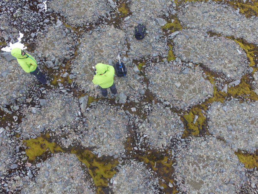
and also on Mars [3,4], easily attracting the attention due to its remarkable circular geometry (Figure 1).
These metric circular shapes, occurring in clusters of up to thousands of individuals, are constituted by an
inner fine domain of soil surrounded by stone rings ascending few centimetres above its interior. This
radial segregation of the geological material according to size (named sorting) is performed at the surface
after the upward swelling of the soil in the active layer of permafrost in seasonal freezing and thawing
cycles [1,5,6].
Their characterization and monitoring can provide useful information about the underlying processes
if circles are currently active [7,8] and also about the past climatic conditions that allowed their
formation/evolution [9–13]. In addition, besides their evident geomorphic importance and their use
as paleoclimatic indicators, the periodic burial and exhumation of geological materials may also play
an important role in the soil carbon cycle in connection to permafrost conditions [6]. Although the
processes underlying their formation and evolution are relatively well understood [14–18], their geometric
characteristics, dating, and seasonal dynamics are mainly supported by sampling and monitoring few
Remote Sens. 2020, 12, 160; doi:10.3390/rs12010160 www.mdpi.com/journal/remotesensing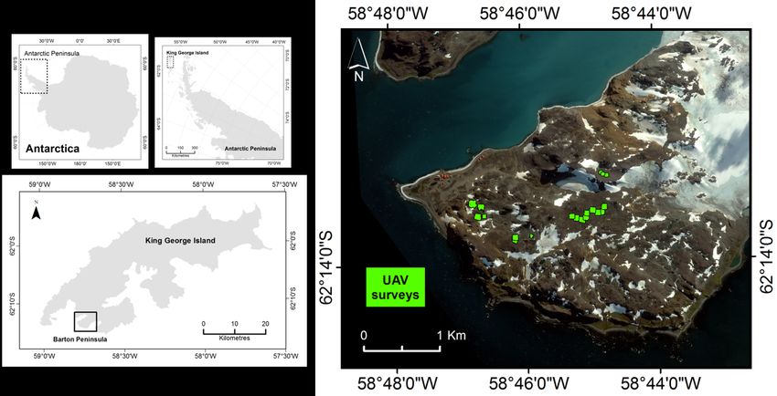
Remote Sens. 2020, 12, 160                                                                               2 of 15

circles in the field [6,11], preventing obtaining robust statistics and an extended spatial analysis of
large fields.

                                         Figure 1. Sorted stone circles.

     Ultra high-resolution imagery (mm to cm) captured by unmanned aerial vehicles (UAV) can greatly
contribute to a much more complete geomorphic description of this type of patterned ground in large
areas, which cannot be perceived in current sub-metric satellite imagery, giving also context to data built
at ground-level [11,19]. The use of UAV in polar regions, and particularly in Antarctica, is becoming a very
important tool for many studies due to the possibility of gathering data on these less accessible regions
with unprecedented detail. Although field operations can be easily constrained by weather conditions,
the diversity of applications is widening fast, encompassing for instance, glacial retreat quantification [20],
landforms mapping [21], vegetation mapping [22] and health state assessment [23], or wildlife inventorying
and monitoring [24], just to name some of the most recent ones. In what concerns their use for studying
stone circles, it is a topic we have started addressing recently [25] and which, as far as we know, has not
been studied before using remote sensing.
     In addition, the large amount of circles to detect requires the use of automated methods to make their
segmentation, characterization and also the multitemporal monitoring to account for the dynamics of
the processes involved. This paper deals now with the initial phase, that is, with the identification and
delineation of the stone circles. However, the detection of circular patterns is a classic pattern recognition
problem using, for instance, popular methods such as template matching and the Hough transform [26,27].
These approaches, requiring the pre-definition of templates to compute the associated voting scheme,
are not the most adequate to deal with the stone circles, as they are not able to take into account the
natural deformation these circular patterns can exhibit. The use of other methods that can deal with more
than slight deformations is therefore the right choice. Thus, we use a pair of such methods, based on the
sliding band filter [28] and on dynamic programming [29–31], which we compare to a traditional template
matching method.
     Thus, this paper aims at detecting sorted stone circles and delineating its boundaries in elevation data
derived from imagery acquired by a UAV in Antarctica. It extends the preliminary work presented in [25]
by considering:

•     the delineation of the stone circle contour;
•     an additional method based on dynamic programming;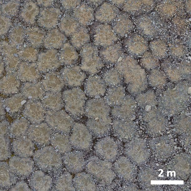
Remote Sens. 2020, 12, 160                                                                                       3 of 15

•     the evaluation of detection and delineation problems in an extended dataset.

2. Image Acquisition

2.1. Study Area
      The sites selected for developing the surveys are located in the ice-free areas of Barton Peninsula
(62◦ 14’S; 58◦ 46’W) in King George Island, the largest one of the South Shetlands in Antarctica (Figure 2 left).
This peninsula has an area of about 10 km2 that started to be exposed about 8000 years ago after glacial
retreat [32]. It shows a rugged topography, with a wide and gentle slope in the central area, ranging from
about 90 to 190 m a.s.l., where the majority of stone circles fields are found [33]. It is also one of the regions
in Antarctica where sorted stone circles are more ubiquitous and therefore an adequate location to study
such type of patterned ground.

      Figure 2. Barton Peninsula in King George Island (left) and location of the UAV survey sites in 2018 plotted
      over a WorldView 2 satellite image (right).

2.2. UAV Surveys
     The surveys were developed during February 2018 in the frame of a field campaign with logistics
support from the Portuguese Polar Program (PROPOLAR) and the Korean Polar Research Institute
(KOPRI). The aerial flights were conducted with a quadcopter DJI Phantom 3 (SZ DJI Technology Co., Ltd.,
Shenzhen, Guangdong, China) equipped with an RGB camera (12 Mpixel, lens 35 mm equivalent, f/2.8) in
the locations of Barton Peninsula where sorted stone circles have the most extended occurrence (Figure 2,
right). They were developed at a low altitude (10 m above ground) to allow perceiving stones down
to 5 mm in size. Each flight was planned in a double-grid mode with high lateral and frontal overlaps
between adjacent images (80%) to provide an increased number of views for the same point. The area
surveyed in each individual flight was conditioned by battery duration reaching up to 80 m × 80 m and
acquiring up to 500 images.

2.3. Mosaic and DEM Construction
    The set of images captured in each flight were processed with Agisoft Photoscan software (version 1.4,
Agisoft LLC, St. Petersburg, Russia) to build an orthorrectified image mosaic and a digital elevation model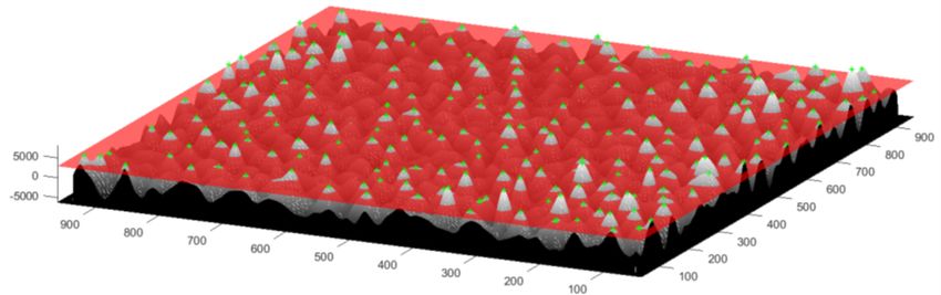
Remote Sens. 2020, 12, 160                                                                                     4 of 15

(DEM), using ground control points measured with a D-GPS to provide accurate georreferencing. The main
procedures underlying the construction of the two products are based on SIFT (Scale-Invariant Feature
Transform) to detect the same feature in adjacent images, RANSAC (Random Sample Consensus) method
to filter erroneous matches and SfM (Structure from Motion) technique to estimate the 3D geometry of the
scene [34]. An example of such product is presented in Figure 3.
      There are small variations in the spatial resolutions of the final mosaic and DEM from site to site due
to the natural fluctuations in position of the UAV along the development of the aerial surveys. The spatial
resolution for all mosaics is in the range of 2.6–3.2 mm/pixels, while, for all DEMs, is in 2.1–2.4 cm/pixel.
These variations in resolution are small and thus can be considered negligible for the generic application
of detection methods. However, only the DEM were used in this work, as the geometric information
provided is the most relevant to detect and delineate the circles. The use of RGB color information can
be more difficult to interpret since color is not directly related to geometry. However, RGB information
may be helpful to solve ambiguous situations, when the transitions between the geological materials of
the circles and background have a poor expression. On the contrary, if vegetation also occurs with the
patterned ground, namely mosses surrounding the circles or lichens on top of the their stones (which does
not happen in all field sites), some additional information (edges) can be used and therefore improve the
performances. This approach deserves being exploited in the future.
      The image mosaics will be also used to analyze other features like, for instance, the size of the stones
or the type of associated vegetation [35].

              Figure 3. Detail of an orthorrectified mosaic (left) and respective shaded relief DEM (right).

3. Methods
     This paper addresses two main problems: the detection of stone circles in elevation data and
the delineation of the contour of each circle. The first problem will be tackled by three methods:
template matching (TM), sliding band filter (SBF), and dynamic programming (DP). The second problem
(contour delineation) is discussed later (Section 3.4), but, as we will see in the following, the last two
methods (SBF and DP) implicitly solve the delineation problem as an intermediate step.

3.1. Template Matching (TM)
     The patterns to be detected mostly have a circular shape with a size approximately constant within
each site (Figure 4, left). Their dimension, which may change a bit in the field from site to site, depends on
some local features, namely the depth of the active layer of permafrost and the characteristics of the soils.
Remote Sens. 2020, 12, 160 5 of 15
We assume that the elevation image contain 3D patterns of known shape T ( x, y), which is denoted as
template. The fit between the elevation image I ( x, y) and the template T ( x, y) that slides along the whole
image can be computed through the correlation
R ( x0 , y0 ) = ∑ I ( x, y) T ( x − x0 , y − y0 ), (1)
( x,y)
which reaches a local maximum when the template and the circle are aligned with each other. The template
that better describes the stone circles is a half-torus (Figure 4, right) described by
+
(r − R )2
q
T ( x, y) = 1− , r= x 2 + y2 , (2)
(eR)2
where R is the radius, eR is the torus width (e = 0.2), and x + = max(0, x ) is the rectifier function.
Figure 4. Stone circle elevation model (left) and half-torus template (right).
The detection of the stone circles is based on the analysis of the correlation matrix R( x, y) by detecting
all the local maxima (non-maximum suppression), followed by a comparison with a threshold Th (Figure 5).
Since the elevation image normally has some natural slope, the image I is first pre-processed by a
high-pass filter to level it.
Figure 5. Threshold of the template matching score as a function of the circle centre.
3.2. Sliding Band Filter (SBF)
The gradient field of natural circles exhibits radial vector patterns (Figure 6). To detect such patterns,
we adopt a modified version of the sliding band filter (SBF) proposed in [28] for the detection of cells in
microscopy images. The problem we are addressing now is slightly different. The gradient of cell images
points inwards while the gradient of stone circles points inwards and outwards, depending on the distance
to the centre.Remote Sens. 2020, 12, 160 6 of 15
Let us assume that we know the centre of the circle c = [ x, y] T and let us define N radial directions
starting from c, with angles θi = 2πi/N, i = 0, . . . , N − 1. Along each direction, we will measure the
alignment between the gradient direction and the radial orientation θi , given by
Ai (r ) = cos(φi (r ) − θi ), (3)
where φi (r ) denotes the direction of the gradient field at a point c + r [cos(θi ), sin(θi )] T . The gradient
orientation changes when the point is located at the circle boundary. To detect the boundary, we will
perform template matching along each direction and choose the radius r0 that corresponds to the highest
peak. Therefore, the best alignment in direction θi is
( )
Ai = max
r0
∑ T (r − r0 ) A i (r ) , (4)
r
where T = u(r + ∆) − 2u(r ) + u(r − ∆) is the template (u(r ) that denotes the unit step signal). Since there
are N radial directions, the global alignment is the sum of all the directional alignments
N −1
A= ∑ Ai . (5)
i =0
These equations provide the alignment score associated with the centre hypothesis c = [ x, y] T .
However, since, in practice, we do not know c, we compute the alignment score for each image point c and
detect the circle centers through non-maximum suppression and thresholding.
The gradient vector is computed with Sobel masks and its magnitude is compared to a threshold:
gradients with small magnitude are discarded.
Figure 6. Gradient fields of natural stone circle (left) and torus (right).
3.3. Dynamic Programming (DP)
The sliding band filter finds the best alignment in each direction θi , according to Equation (4). This is a
sub-optimal approach and often leads to abrupt transitions of the radius at consecutive directions. To overcome
this difficulty, we will perform a joint estimation of the contour points at all the directions, using dynamic
programming (DP).
First, we will discretize the polar coordinates as follows:
angle: i∆θ, i = 0, . . . , N − 1,
(6)
radius: rmin + r∆r, r = 0, . . . , M − 1.Remote Sens. 2020, 12, 160 7 of 15
A contour is represented as a sequence of radius variables r0 , . . . , r N −1 . Since the contour is closed,
we will extend the sequence with an additional variable r = (r0 , . . . , r N ) and assume that r0 = r N .
In addition, two types of penalties will be considered: the alignment cost at direction i and radius r,
inspired in the SBF alignment,
Ci (r ) = − ∑ T ( p − r ) Ai ( p), (7)
p
and the transition cost (
0 β |r − r 0 |, |r − r 0 | ≤ m,
c(r, r ) = (8)
∞, otherwise,
which becomes infinite if the radius difference exceeds a threshold: |r − r 0 | > m.
Therefore, the total cost E associated with a contour starting at r0 = k and ending at r N = k is given
by the quantity
N
E(r) = ∑ Ci (ri ) + c(ri−1 , ri ), r0 = r N = k. (9)
i =1
The minimization of E(r), under the constraint r0 = r N = k can be efficiently solved by dynamic
programming [36,37]. This procedure involves two steps which are known as forward recursion and
backward recursion.
The forward recursion computes the optimal cost to go from the direction 0 and radius k to the
direction t and radius j
" #
t
Et ( j) = min
r1 ,...,rt :rt = j
∑ Ci (ri ) + c(ri−1 , ri ) , r0 = k. (10)
i =1
The optimal costs can be recursively computed in an efficient way through
Et ( j) = Ct ( j) + min [ Et−1 (r ) + c(r, j)] . (11)
r
Since we also want to retrieve the optimal path, we need to store the value of r that minimizes
[ Et−1 (r ) + c(r, j)]. This is done by defining a set of pointers
φt ( j) = arg min [ Et−1 (r ) + c(r, j)] , j = 0, . . . , M − 1. (12)
r
After computing Et ( j), φt ( j), t = 1, . . . , N, the optimal contour can be recovered by backtracking.
The backward recursion is initialized as r ∗N = k. Then, we recursively compute
rt∗−1 = φ(rt∗ ), t = N, . . . , 1 (13)
The algorithm with the constraints r0 = r N = k is summarized in Table 1. It finds the optimal path
under the constraint r0 = k. Since we do not know the best initial radius k, all the k values should be tested
and the best (the one that minimizes E) should be chosen. However, this approach is computationally
heavy, therefore we have adopted a faster algorithm based on two repetitions only, as proposed in [29].Remote Sens. 2020, 12, 160 8 of 15
Table 1. Dynamic Programming algorithm with constraints r0 = r N = k.
E0 ( j) = 0
Forward Recursion Et ( j) = Ct ( j) + minr [ Et−1 (r ) + c(r, j)] , t = 1, 2, . . . , N,
φt ( j) = arg minr [ Et−1 (r ) + c(r, j)] , t = 1, 2, . . . , N.
r ∗N = k
Backward Recursion
rt∗−1 = φ(rt∗ ), t = N, N − 1, . . . , 1
The minimum value of E is a score that measures how well the image patch considered can be fitted
by a smooth contour. It is, therefore, a score that can be used for the detection of the stone circles. In a
typical application, the patch slides along the image. Every image pixel is considered to be the centre of a
stone circle being the detection obtained by non-minimum suppression followed by thresholding.
3.4. Contour Delineation
The SBF and DP methods provide an estimate of the stone circle contour in polar coordinates.
Therefore, nothing else has to be done to delineate the object contour.
In SBF, each contour point is independently obtained by the maximization of the filtered alignment
along each radial direction Equation (4). In the DP method, the contour is the output of a joint minimization
of all the contour points performed by dynamic programming. The extraction of the contour corresponds
to the backtracking step of the DP algorithm.
4. Results
4.1. Datasets
The datasets used for detecting and delineating the stone circles were obtained by the authors in
Antarctica (Section 2.2). These images contain the natural variability found in the field related to several
circle features, namely, dimension, circularity, ring thickness, and height and degree of completeness.
The detection dataset is constituted by 20 elevation images of 1000 × 1000 pixels extracted from
the larger DEMs built in each site, whereas the delineation dataset is constituted by 24 individual circles
extracted from the previous dataset.
4.2. Performance Evaluation
The evaluation of the performances of detection and delineation algorithms is performed separately
with each of their own metrics.
For the detection algorithms, ground truth (GT) information was built by detecting visually all
the circles in each DEM image and annotating manually their centers using an image analysis software
(MATLAB, version 9.6 (2019a), MathWorks, Natick, Massachusetts, USA). The algorithms also identify a
set of centers, so we need to establish a correspondence between the detected and ground truth centers.
This was achieved through a simple matching algorithm defined as follows. First, we build a matrix
of distances from all the GT centers to all the detected centers. The minimum element of the matrix is
found (excluding the diagonal elements) and the corresponding points are matched, provided that their
minimum distance is smaller than a given threshold ∆. If two points are matched, they are considered a
true positive (TP) detection and the corresponding line and column are removed from the distance matrix.
The process is repeated until there are no more candidates for matching. The ground truth points not
matched are considered false negatives (FN), and the detected points that were not matched are considered
false positives (FP).Remote Sens. 2020, 12, 160 9 of 15
The performance of the detection algorithm is obtained through the well known measures
TP TP
Precision = , Recall = . (14)
TP + FP TP + FN
The Precision and Recall combined provide the single measure F-score
Precision.Recall
F-score = 2 . (15)
Precision + Recall
For the delineation algorithms, the evaluation is performed through the comparison of the delineated
contour with a ground-truth contour that is, a manually drawn contour. For computing the distortion
between each pair of contours, we adopt the approach used in a similar delineation problem [38], assuming
that the detected contour should be within a band of a given width ∆ around the ground-truth contour.
This way, points located outside this band are considered errors, with their percentage used as a measure
of distortion between both contours.
Let A denote the set of boundary points detected by the delineation algorithm, and let B denote
the ground-truth boundary defined by an expert. We define the distance from a point p ∈ A to the
ground-truth contour B as the distance from p to the nearest point q in B
d( p, B) = min k p − qk. (16)
q∈ B
The amount of errors is given by the following equation:
1
E∆ =
#A ∑ δ(d( p, B) ≥ ∆), (17)
p∈ A
where #A is the number of points of set A; δ( x ) = 1 if x = true, and δ( x ) = 0 if otherwise.
We have chosen for this study ∆ = 0.15R, where R is the stone circle radius. If d( p, B) = 0, the point
p is assumed to be correct, and there is no error (cp). If 0 ≤ d( p, B) ≤ ∆, the error in p is considered a small
error (se), and if d( p, B) ≥ ∆, p is considered a gross error (ge).
4.3. Detection
The detection algorithms were tested, assuming different configurations for their parameters. To be
specific, the three parameters for TM method are R (radius of template), e (template width) and
Th (threshold), which were tested with the configurations: R ∈ {25, 30, 35, 40}, e ∈ {0.1, 0.2, 0.3, 0.4}
and Th ∈ {25, 30, 35, 40, 45, 50, 55}. The SBF method encompasses two parameters concerning
N (number of directions) and Th (threshold) whose tested configurations were: R ∈
{16, 32, 64, 128}, and Th ∈ {60, 65, 70, 75, 80}. Finally, the four parameters for DP method, which are
N (number of directions), Th (threshold), β (transition cost) and m (maximum transition allowed), were
evaluated with the configurations: N ∈ {16, 32, 64, 128}, Th ∈ {60, 65, 70, 75, 80}, β ∈ {0, 0.03, 3} and
m ∈ {1, 3, 5, 10}.Remote Sens. 2020, 12, 160 10 of 15
All combinations of configurations for each method were evaluated with the metrics defined above.
Those achieving the highest F-scores, among all combinations, are the following:
• TM: R = 30 pixels, e = 0.4, Th = 35%.
• SBF: N = 128, Th = 80%.
• DP: N = 128, Th = 65%, β = 1, m = 1.
The outputs of each method with the optimal parameters are illustrated with three different images
in Figure 7.
These results show the ability of automatic methods to detect stone circles. The TM method performs
worse than SBF and DP, since it has more false positive detections. The best method is DP, but the difference
with respect to SBF is small. It can also be observed that the performance of the automatic detectors is
better in the first and third examples (left and right columns) than in the second (middle column) where
the circles have stronger deformations and exhibit a less uniform spatial distribution pattern.
Table 2 shows the detection scores (precision, recall and F-score). Not unexpectedly, DP and SBF
methods achieve the highest average F-scores with 85.2% and 82.0%, respectively, clearly outperforming
TM method with 66.7%. This difference derives from TM making a strong rigidity assumption about
the shape of the circles while SBF and DP are flexible and make appropriate trade-offs between shape
and deformation.
Table 2. Detection performances: mean and standard deviation for template matching (TM), sliding band
filter (SBF) and dynamic programming (DP) methods.
Method Parameters Precision (%) Recall (%) F Score (%) Time (min)
TM R = 30, e = 0.4, Th = 35 63.1 (11.7) 72.7 (10.1) 66.7 (8.9) 0.1 (0.1)
N = 128, Th = 80 82.2 (14.5) 84.2 (8.8) 82.0 (6.6) 14.9 (1.0)
SBF
N = 16, Th = 80 81.3 (14.4) 83.9 (4.1) 81.3 (6.9) 1.8 (0.2)
N = 128, Th = 65, β = 3, m = 1 85.2 (6.6) 85.5 (14.8) 85.2 (6.6) 23.9 (12.9)
DP
N = 16, Th = 65, β = 0.03, m = 1 87.0 (8.1) 80.7 (8.4) 84.3 (6.1) 3.6 (1.6)
Nevertheless, the much larger average computation time per image of DP and SBF methods (23.9 and
14.9 min, respectively) when compared to TM (0.1 min) requires their evaluation under less restrictive
conditions. Just decreasing the number of directions of analysis in each method from 128 to 16 turns the
computation time to be only 15% and 12% of the initial duration for DP and SB, respectively, and still
keeping the F-score performances at a high level: 84.3% for DP and 81.3% for SBF.Remote Sens. 2020, 12, 160 11 of 15
Figure 7. Detection outputs from three field sites, from top to bottom in each column: initial image, TM,
SBF, and DP. The colored markers mean: TP (green), FP (red) and FN (yellow).Remote Sens. 2020, 12, 160 12 of 15
4.4. Delineation
The delineations performed by each method are illustrated in Figure 8. Both methods find the contour
of the stone circles, but DP leads to smoother contours since it performs a global estimation of the contour
and has less gross errors.
The delineation does not always provide an accurate contour. Two examples are shown in Figure 9
in which SBF and DP fail. In the first case (SBF), there are strong elevation artefacts that produce
spurious detections in some directions. In the second case (DP), the shape of the contour can no longer be
approximated by a circle and the shape model (circle) does not fit the image.
Table 3 shows the performances achieved by each method in the whole dataset of circles.
The evaluation is based on gross errors only, since we consider small errors to be acceptable. Although both
methods perform well, DP clearly outperforms SBF, with gross errors of 7.1% and 18.3%, respectively.
On the contrary, the average computation time for each individual circle with DP (50.2 s) is almost ten
times slower than SBF (5.5 s).
This difficulty can be overcome by substantially decreasing the number of directions (from 360
to 64). This change has, similarly to the detection problem, a strong effect on the reduction of the average
computation time of DP method with almost no effect on the quality of its delineations: it is more
than 15 times faster (from 50.2 to 3.2 s), keeping gross errors practically unchanged (from 7.1% to 7.2%).
Although less significant, there is also an average computation time reduction for SBF (from 5.5 to 4.4 s)
but now with a slight decrease of gross errors (from 18.3% to 18.0%).
Figure 8. Delineation outputs in two circles, from left to right in each row: initial image, SBF and DP.
The green line corresponds to the ground-truth while the coloured circles designate cp (green), se (yellow)
and ge (red).Remote Sens. 2020, 12, 160 13 of 15
Figure 9. Delineation failures in two examples by SBF (left) and DP (right). The colors have the same
meaning as indicated in Figure 8.
Table 3. Delineation performances: mean and standard deviation for correct points (cp), gross errors (ge)
and small errors (se) for sliding band filter (SBF) and dynamic programming (DP) methods.
Method Parameters cp (%) se (%) ge (%) Time (s)
N = 360 21.4 (9.4) 60.4 (11.7) 18.3 (18.8) 5.5 (1.8)
SBF
N = 64 18.5 (8.5) 63.5 (13.0) 18.0 (18.8) 4.4 (1.3)
N = 360, β = 3 m = 1 27.6 (9.8) 65.3 (10.6) 7.1 (12.3) 50.2 (14.3)
DP
N = 64, β = 0.3 m = 1 24.6 (10.3) 68.2 (13.0) 7.2 (13.7) 3.2 (0.8)
5. Conclusions
This paper provides new advances for the study of sorted stone circles through automated methods
applied to elevation maps built from UAV surveys. Three methods were proposed for circle detection
(template matching, sliding band filter, and dynamic programming) with the last two being also used for
contour delineation.
Good results were obtained by the sliding band filter and dynamic programming methods, both in
the detection and delineation problems. However, the dynamic programming method performs better in
both problems. An F-Score of 85.2% was achieved in a database of 20 elevation maps. In the delineation
problem, a percentage of 7.1% of gross errors was obtained, being all the other points correctly estimated.
The flexibility inherent to sliding band filter and dynamic programming detection methods makes
them a good option to deal with the natural variability associated with the stone circles, since they
can encompass variations in their circularity, thickness, and height of the stone ring and also in their
percent completeness.
For future work, we intend to exploit the use of the RGB images to improve the performances and
also to apply other methods (e.g., deep leaning) to the detection and delineation of the stone circles. These
methods require the enlargement of the datasets, which will be achieved after the development of more
UAV surveys in other ice-free regions of Antarctica.
Author Contributions: All authors contributed to the development and testing of the methodologies and to writing
the manuscript. P.P. and S.H. developed the field surveys in Antarctica. All authors have read and agreed to the
published version of the manuscript.
Funding: The research presented in this paper was funded by the Portuguese Polar Program (PROPOLAR)
through research campaign projects CIRCLAR2 in 2017–2018 and the pluriannual funding projects of CERENA
(UID/ECI/04028/2019) and ISR (UID/EEA/50009/2019) funded by FCT—Fundação para a Ciência e a Tecnologia.Remote Sens. 2020, 12, 160 14 of 15
Acknowledgments: The support at King Sejong Station and field logistics in Barton Peninsula provided by the Korean
Polar Research Institute (KOPRI) and the logistical support by the Portuguese Polar Program (PROPOLAR) are
warmly thanked.
Conflicts of Interest: The authors declare no conflict of interest.
References
1. Washburn, A.L. Geocryology: A Survey of Periglacial Processes and Environments; Wiley: New York, NY, USA, 1980.
2. Hallet, B.; Prestrud, S. Dynamics of periglacial circles in Western Spitsbergen. Quat. Res. 1986, 26, 81–99.
[CrossRef]
3. Balme, M.R.; Gallagher, C.J.; Page, D.P.; Murray, J.B.; Muller, J.-P. Sorted stone circles in Elysium Planitia, Mars:
Implications for recent martian climate. Icarus 2009, 200, 30–38. [CrossRef]
4. Gallagher, C.; Balme, M.R.; Conway, S.J.; Grindrod, P.M. Sorted clastic stripes, lobes and associated gullies in
high-latitude craters on Mars: Landforms indicative of very recent, polycyclic ground-ice thaw and liquid flows.
Icarus 2011, 211, 458–471. [CrossRef]
5. Hallet, B. Stone circles: Form and soil kinematics. Philos. Trans. R. Soc. A 2013, 371, 20120357. [CrossRef]
[PubMed]
6. Kaab, A.; Girod, L.; Berthling, I. Surface kinematics of periglacial sorted circles using structure-from-motion
technology. Cryosphere 2014, 8, 1041–1056. [CrossRef]
7. Kasprzak, M. High-resolution electrical resistivity tomography applied to patterned ground, Wedel Jarlsberg
Land, south-west Spitsbergen. Polar Res. 2015, 34, 25678. [CrossRef]
8. Slee, A.; Kiernan, K.; Shulmeister, J. Contemporary sorted patterned ground in low altitude areas of Tasmania.
Geogr. Res. 2015, 53, 175–183. [CrossRef]
9. Cox, G.W.; Allen, D.W. Sorted stone nets and circles of the Columbia Plateau: A hypothesis. Northwest Sci. 1987,
16, 179–185.
10. Etzelmüller, B.; Sollid, J.L. The role of weathering and pedological processes for the development of sorted circles
on Kvadehuksletta, Svalbard—A short report. Polar Res. 1991, 9, 181–191. [CrossRef]
11. Jeong, G.Y. Radiocarbon ages of sorted circles on King George Island, South Shetland Islands, West Antarctica.
Antarct. Sci. 2006, 18, 265–270. [CrossRef]
12. Křížek, M.; Uxa, T. Morphology, sorting and microclimates of relict sorted polygons, Krkonoše Mountains, Czech
Republic. Permafr. Periglac. Process. 2013, 24, 313–321. [CrossRef]
13. Uxa, T.; Mida, P.; Křížek, M. Effect of climate on morphology and development of sorted circles and polygons.
Permafr. Periglac. Process. 2017, 28, 663–674. [CrossRef]
14. Kessler, M.A.; Murray, A.B.; Werner, B.T.; Hallet, B. A model for sorted circles as self-organized patterns.
J. Geophys. Res. Solid Earth 2001, 106, 13287–13306. [CrossRef]
15. Kessler, M.A.; Werner, B.T. Self-organization of sorted patterned ground. Science 2003, 299, 380–383. [CrossRef]
[PubMed]
16. Holness, S.D. Sorted circles in the Maritime Sub-Antarctic, Marion Island. Earth Surf. Process. Landforms 2003, 28,
337–347. [CrossRef]
17. Haugland, J.E. Formation of patterned ground and fine-scale soil development within two late Holocene glacial
chronosequences: Jotunheimen, Norway. Geomorphology 2004, 61, 287–301. [CrossRef]
18. Yamagishi, C.; Matsuoka, N. Laboratory frost sorting by needle ice: A pilot experiment on the effects of stone
size and extent of surface stone cover. Earth Surf. Process. Landforms 2015, 40, 502–511. [CrossRef]
19. Pina, P.; Vieira, G.; Bandeira, L.; Mora, C. Accurate determination of surface reference data in digital photographs
in ice-free surfaces of Maritime Antarctica. Sci. Total Environ. 2016, 573, 290–302. [CrossRef]
20. Pudełko, R.; Angiel, P.J.; Potocki, M.; J˛edrejek, A.; Kozak, M. Fluctuation of glacial retreat rates in the eastern part
of Warszawa Icefield, King George Island, Antarctica, 1979–2018. Remote. Sens. 2018, 10, 892.Remote Sens. 2020, 12, 160 15 of 15
21. Dabski, M.; Zmarz, A.; Pabjanek, P.; Korczak-Abshire, M.; Karsznia, I.; Chwedorzewska, K.J. UAV-based
detection and spatial analyses of periglacial landforms on Demay Point (King George Island, South Shetland
Islands, Antarctica). Geomorphology 2018, 290, 29–38. [CrossRef]
22. Miranda, V.; Pina, P.; Heleno, S.; Vieira, G.; Mora, C.; Schaefer, C.E.G.R. Monitoring recent changes of
vegetation in Fildes Peninsula (King George Island, Antarctica) through satellite imagery guided by UAV surveys.
Sci. Total Environ. 2020, 704, 135295. [CrossRef] [PubMed]
23. Turner, D.; Lucieer, A.; Malenovský, Z.; King, D.; Robinson, S.A. Assessment of Antarctic moss health from
multi-sensor UAS imagery with random forest modelling. Int. J. Appl. Earth Obs. Geoinf. 2018, 68, 168–179.
[CrossRef]
24. Korczak-Abshire, M.; Zmarz, A.; Rodzewicz, M.; Kycko, M.; Karsznia, I.; Chwedorzewska, K.J. Study of
fauna population changes on Penguin Island and Turret Point Oasis (King George Island, Antarctica) using an
unmanned aerial vehicle. Polar Biol. 2019, 42, 217–224. [CrossRef]
25. Pina, P.; Pereira, F.; Marques, J.S.; Heleno, S. Detection of stone circles in periglacial regions of Antarctica in UAV
datasets. In Pattern Recognition and Image Analysis; Morales, A., Fierrez, J., Sánchez, J., Ribeiro, B., Eds.; Lecture
Notes in Computer Science; Springer: Cham, Switzerland, 2019; Volume 11867, pp. 279–288.
26. Yuen, H.K.; Princen, J.; Illingworth, J.; Kittler, J. Comparative study of Hough Transform methods for
circle finding. Image Vis. Comput. 1990, 8, 71–77. [CrossRef]
27. Mukhopadhyay, P.; Chaudhuri, B.B. A survey of Hough Transform. Pattern Recognit. 2015, 48, 993–1010.
[CrossRef]
28. Quelhas, P.; Marcuzzo, M.; Mendonça, A.M.; Campilho, A. Cell nuclei and cytoplasm joint segmentation using
the sliding band filter. IEEE Trans. Med Imaging 2010, 29, 1463–1473. [CrossRef]
29. Dias, J.M.B.; Leitão, J.M.N. Wall position and thickness estimation from sequences of echocardiographic images.
IEEE Trans. Med Imaging 1996, 15, 25–38. [CrossRef]
30. Marques, J.S.; Pina, P. Crater delineation by dynamic programming. IEEE Geosci. Remote. Sens. Lett. 2015, 12,
1581–1585. [CrossRef]
31. Santiago, C.; Nascimento, J.C.; Marques, J.S. Fast segmentation of the left ventricle in cardiac MRI using dynamic
programming. Comput. Methods Programs Biomed. 2018, 154, 9–23. [CrossRef]
32. Oliva, M.; Antoniades, D.; Serrano, E.; Giralt, S.; Liu, E.J.; Granados, I.; Pla-Rabes, S.; Toro, M.; Hong, S.G.;
Vieira, G. The deglaciation of Barton Peninsula (King George Island, South Shetland Islands, Antarctica) based
on geomorphological evidence and lacustrine records. Polar Rec. 2019, 55, 177–188. [CrossRef]
33. López-Martínez, J.; Serrano, E.; Schmid, T.; Mink, S.; Linés, C. Periglacial processes and landforms in the South
Shetland Islands (northern Antarctic Peninsula region). Geomorphology 2012, 155–156, 62–79. [CrossRef]
34. Smith, M.W.; Carrivick, J.L.; Quincey, D.J. Structure from motion photogrammetry in physical geography.
Prog. Phys. Geogr. 2016, 40, 247–275. [CrossRef]
35. Calviño-Cancela, M.; Martín-Herrero, J. Spectral discrimination of vegetation classes in ice-free areas of Antarctica.
Remote. Sens. 2016, 8, 856. [CrossRef]
36. Geiger, D.; Gupta, A.; Costa, L.A.; Vlontzos, J. Dynamic Programming for detecting, tracking, and matching
deformable contours. IEEE Trans. Pattern Anal. Mach. Intell. 1995, 17, 294–302. [CrossRef]
37. Amini, A.A.; Weymouth, T.E.; Jain, R.C. Using Dynamic Programming for solving variational problems in vision.
IEEE Trans. Pattern Anal. Mach. Intell. 1990, 12, 855–867. [CrossRef]
38. Marques, J.S.; Pina, P. An algorithm for the delineation of craters in very high resolution images of Mars surface.
In Pattern Recognition and Image Analysis; Sanches, J.M., Micó, L., Cardoso, J.S., Eds.; Lecture Notes in Computer
Science; Springer: Berlin/Heidelberg, Germany, 2013; Volume 7887, pp. 213–220.
c 2020 by the authors. Licensee MDPI, Basel, Switzerland. This article is an open access
article distributed under the terms and conditions of the Creative Commons Attribution
(CC BY) license (http://creativecommons.org/licenses/by/4.0/).You can also read