Copernicus Global Land Cover Layers-Collection 2 - MDPI
←
→
Page content transcription
If your browser does not render page correctly, please read the page content below
remote sensing
Communication
Copernicus Global Land Cover Layers—Collection 2
Marcel Buchhorn 1, * , Myroslava Lesiv 2 , Nandin-Erdene Tsendbazar 3 , Martin Herold 3 ,
Luc Bertels 1 and Bruno Smets 1
 1    Remote Sensing Unit, Flemish Institute for Technological Research (VITO), B-2400 Mol, Belgium;
      luc.bertels@vito.be (L.B.); Bruno.smets@vito.be (B.S.)
 2    Ecosystems Services and Management, International Institute for Applied Systems Analysis (IIASA),
      A-2361 Laxenburg, Austria; lesiv@iiasa.ac.at
 3    Laboratory of Geo-Information Science and Remote Sensing, Wageningen University & Research,
      NL-6708 Wageningen, The Netherlands; nandin.tsendbazar@wur.nl (N.-E.T.); martin.herold@wur.nl (M.H.)
 *    Correspondence: marcel.buchhorn@vito.be

 Received: 19 February 2020; Accepted: 22 March 2020; Published: 24 March 2020

 Abstract: In May 2019, Collection 2 of the Copernicus Global Land Cover layers was released. Next to
 a global discrete land cover map at 100 m resolution, a set of cover fraction layers is provided
 depicting the percentual cover of the main land cover types in a pixel. This additional continuous
 classification scheme represents areas of heterogeneous land cover better than the standard discrete
 classification scheme. Overall, 20 layers are provided which allow customization of land cover maps
 to specific user needs or applications (e.g., forest monitoring, crop monitoring, biodiversity and
 conservation, climate modeling, etc.). However, Collection 2 was not just a global up-scaling, but also
 includes major improvements in the map quality, reaching around 80% or more overall accuracy.
 The processing system went into operational status allowing annual updates on a global scale with an
 additional implemented training and validation data collection system. In this paper, we provide an
 overview of the major changes in the production of the land cover maps, that have led to this increased
 accuracy, including aligning with the Sentinel 2 satellite system in the grid and coordinate system,
 improving the metric extraction, adding better auxiliary data, improving the biome delineations,
 as well as enhancing the expert rules. An independent validation exercise confirmed the improved
 classification results. In addition to the methodological improvements, this paper also provides an
 overview of where the different resources can be found, including access channels to the product
 layer as well as the detailed peer-review product documentation.

 Keywords: Copernicus; land use/cover classification; cover fractions;                  remote sensing;
 global land cover mapping; random forest; time series analysis

1. Introduction
     Land is an important asset for human beings. The globalization of the world’s economy and the
increase of its population, however, have large environmental consequences and put unprecedented
pressure on land management [1–3]. To understand these consequences and to act upon them,
accurate characterization of land cover and land-use change is essential. This also means records of
vegetation characteristics and land cover (LC) need to be available. While long-term consistent in
situ observations for large areas remain scarce, satellite remote sensing has become a major source of
information for the monitoring of vegetation dynamics since the 70s [4]. Satellite systems like Landsat,
National Oceanic and Atmospheric Administration’s (NOAA) AVHRR, and MODIS, among others,
provide long-term records of reflectance data on a global scale [5–7]. These datasets have been
used to generate state-of-the-art global discrete LC maps at low to medium resolution [8,9] like
the GlobCover [10], LC-CCI [11], and MODIS [12] products. Gong et al. [13] produced the first

Remote Sens. 2020, 12, 1044; doi:10.3390/rs12061044                      www.mdpi.com/journal/remotesensing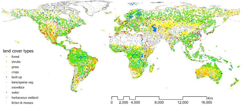
Remote Sens. 2020, 12, 1044                                                                        2 of 14

global high-resolution LC map at 30 m resolution, attaining an overall classification accuracy of 65%.
Nevertheless, all these LC maps have a major drawback—they have fixed legends and therefore rigid
characterization of LC types. Land cover maps are used by various user groups to better understand
the current landscapes and the impact we have as global citizens. But at the same time, these LC maps
are often hard to use in applications that require up-to-date information, such as forest monitoring,
sustainable development goals monitoring, and biodiversity monitoring. The variety in the needs
between all these different users makes it hard to create a one-size-fits-all LC map. More elastic LC
mapping approaches are thus needed to guarantee high-quality products for these users [14].
     As part of the European Copernicus service which aims to provide systematic global monitoring
of the Earth’s land surface, the Copernicus Global Land Service has recently released yearly global LC
maps at 100 m resolution from 2015 onwards [15]. Copernicus’ Global Land Cover product aims to
provide dynamic LC layers that allow creating custom LC maps that fit the needs of different map
users. Therefore, next to a discrete LC map, a set of cover fraction layers is delivered, depicting the
percentual cover of main LC types in a pixel. This allows the user to tailor the LC product to his
application and needs, and to harmonize it to other available LC maps.
     The first Copernicus Global Land Service Land Cover Map at 100 m (CGLS-LC100)—Collection 1—was
provided for the 2015 reference year over the African continent in July 2017. It was derived from
100 m time-series of the vegetation instrument on board of the PROBA satellite (PROBA-V) [16,17],
a database of high-quality LC reference sites and several ancillary datasets. We integrated spectral,
temporal and spatial features derived from the PROBA-V time series to improve classification accuracy
as recommended by Zhai et al. [18] and Eberenz et al. [19]. Based on the success of this demonstration
product for Africa, showing high quality with an overall accuracy of 74.3% and alignment to other
continental LC maps [20–23], Collection 2 of the CGLS-LC100 product was released in May 2019,
extending the map to a global coverage for the reference year 2015 [15]. However, Collection 2 was
not just a global up-scaling, but also includes major improvements in the map quality, reaching now
around 80% or more of overall accuracy for each continent. Further improvements include the switch
from the system World Geodetic System 1984 (WGS84) to the Universal Transverse Mercator (UTM)
coordinate system and the alignment to the Sentinel-2 tiling grid in order to improve mapping quality
in the high latitudes [24]. Moreover, this gridding system facilitates the continuation of the yearly
CGLS-LC100 product when switching from PROBA-V to Sentinel-2 as an input data source.
     The objective of this communication is to introduce potential users to the product, to give a short
overview to the methodology, accuracy assessment, and product comparisons. Moreover, the different
data access channels to the datasets as well as more detailed product documentation are provided.

2. Methodological Overview

2.1. General Overview
     In this section, a broad overview of the CGLS-LC100 production workflow is given. For a more
detailed explanation of the whole workflow, including detailed technical descriptions of algorithms,
used ancillary data, and produced intermediate products, we refer to the Algorithm Theoretical Basis
Document (ATBD) [25].
     It is important to note that the overall workflow used in the Copernicus Global Land Service Land
Cover processing workflow is not sensor-specific, and can be applied to any satellite data, irrespective
of the sensor or resolution (Figure 1). Where sensors like Sentinel-1, Sentinel-2, and Landsat were up to
now mainly used for regional/continental LC mapping applications [26,27], the CGLS-LC100 Collection
2 product uses PROBA-V sensor data, despite the workflow is already tested with Sentinel-2 and
Landsat. The CGLS-LC100 product is generated by combining high-quality external data and several
proven individual methodologies for processing Earth Observation (EO) data (Figure 1). Each of
the workflow blocks in Figure 1, EO data pre-processing, classification/regression pre-processing,
Remote Sens. 2020, 12, 1044                                                                         3 of 14

classification/regression and product generation, and validation and comparison are described in the
sections below.

      Figure 1. Workflow overview for generation of Copernicus Global Land Cover Layers. Adapted from
      the Algorithm Theoretical Basis Document (ATBD) [25].

2.2. EO Data Pre-Processing
      One main improvement in Collection 2 of the GCLS-LC100 product was the reprocessing of
the PROBA-V archive to improve the quality of the EO input data. The complete PROBA-V L1C
archive (unprojected, Top-of-Atmosphere data) was translated into the PROBA-V UTM Analysis
Ready Data (ARD) archive following the recommendations for ARD datasets by Dwyer et al. [28].
The geometric processing included the projection into the UTM coordinate system, fully aligned with
the Sentinel-2 tiling grid in naming as well as tile dimensions [29]. This reduced distortions in the High
North, and will allow continuity of the service beyond the lifetime of the PROBA-V sensor. Through
an improved atmospheric correction, the reflectance values were converted to surface reflectance
(Top-of-Canopy).
      From the PROBA-V UTM ARD, the 5-daily PROBA-V UTM multi-spectral image data with
a Ground Sampling Distance (GSD) of ~0.001 degrees (~100 m), is used as primary EO data,
while PROBA-V UTM daily multi-spectral image data with a GSD of ~0.003 degrees (~300 m)
as a secondary source. In addition to the Status Mask (SM) cleaning for each image, a temporal cloud
and outlier filter was applied to further clean the data, built on a Fourier transformation [30–32]. As a
final step, median compositing was carried out in order to archive regular 5-daily time steps in the
100 m and 300 m PROBA-V EO time series, upgrading the PROBA-V UTM ARD archive into the
PROBA-V UTM ARD+ archive. From this cleaned and outlier screened data, a Data Density Indicator
(DDI) was calculated, which was used as an input quality indicator in the supervised learning process.
      As a final step in the input EO data preparation, to improve the data density in the 5-daily
100 m time series, the 100 m and 300 m EO datasets were fused using a Kalman filtering approach,
Remote Sens. 2020, 12, 1044 4 of 14
based on Sedano et al. [33] and tested by Kempeneers et al. [34], but further adapted to heterogonous
surfaces. This upgraded the PROBA-V UTM ARD+ archive into the PROBA-V UTM ARD++ archive,
containing temporally cleaned, consistent and dense 5-daily image stacks for all global land masses at
100 m resolution.
2.3. Classification/Regression Pre-Processing
A next step is the calculation of the metrics, which are used as general descriptors to enable
distinguishing the different LC classes. The PROBA-V UTM ARD++ archive is used as input for this
metrics generation step. Instead of using the original reflectance values, more descriptive Vegetation
Indices (VI’s) are used (Figure 1). Overall ten VI’s are generated using the four reflectance bands of
PROBA-V, in detail: Normalized Difference Vegetation Index (NDVI), Enhanced Vegetation Index (EVI),
Structure Intensive Pigment Index (SIPI), Normalized Difference Moister Index (NDMI), Near-Infrared
reflectance of vegetation (NIRv), Angle at NIR, HUE, and VALUE of the Hue Saturation Value (HSV)
color system transformation, Area Under the Curve (AUC), and Normalized Area Under the Curve
(NAUC) (for detailed VI’s definition see ATBD [25]). Since the whole time series stack of the VI’s for
an epoch (three years period giving reference year +/- 1 year) would be too many proxies to be used
in supervised learning, the time dimension in the data stack was condensed. Temporal descriptors
were derived through a harmonic model, fitted through the time steps of each of the VI’s based on
a Fourier transformation [30,32]. In addition to the seven parameters of the harmonic model using
three frequencies above the zero-frequency, used as metrics for the overall level and seasonality of the
time series, 11 descriptive statistics (mean, standard deviation, minimum, maximum, sum, median,
10th percentile, 90th percentile, 10th – 90th percentile range, time step of the first minimum appearance,
and time step of the first maximum appearance) and one textural metrics (median variation of center
pixel to median of the neighbors) were generated for each VI. Additionally, four external metrics
including the height, slope, aspect, and purity derived at 100 m were derived from a Digital Elevation
Model (DEM). Overall, 270 metrics were extracted from the PROBA-V UTM ARD++ archive for the
2015 epoch which includes spectral, temporal, and spatial features as suggested by Zhai et al. [18] and
Eberenz et al. [19].
In addition to the input EO data, other data sources were needed as well. Prior to using these
external ancillary data, they were checked for consistency and if needed, re-warped to the UTM
coordinate system, resampled to 100 m, retiled into the Sentinel-2 tiling grid, and post-processed to
usable ancillary data products (Figure 1). Since water surfaces and built-up surfaces are not classified
in the CGLS-LC100 algorithm but fused in from these ancillary data sets, the most important ancillary
dataset in the CGLS-LC100 processing line is JRC’s Global Surface Water dataset [35] and DLR’s World
Settlement Footprint (WSF) [36].
Training data has been collected through the Geo-Wiki engagement platform by a group of
20 experts trained by IIASA staff [37]. Note that the training data collection is not through the use
of volunteer efforts but instead by a group of highly trained experts involved in the data collection.
Therefore, a specific branch of Geo-Wiki, which is only accessible to the experts, has been consolidated
for collecting training data at the required resolution and grid. The training data was collected via a
10x10 grid at 10 m spatial resolution through manual classification using Google Maps and Microsoft
Bing images. Consequently, the training data not only includes the land cover type, but also the cover
fractions of the main LC classes per 100 m resolution cell. Such fractions can be easily translated
into different legends. Here, we used LC definitions as suggested by the United Nations (UN) Land
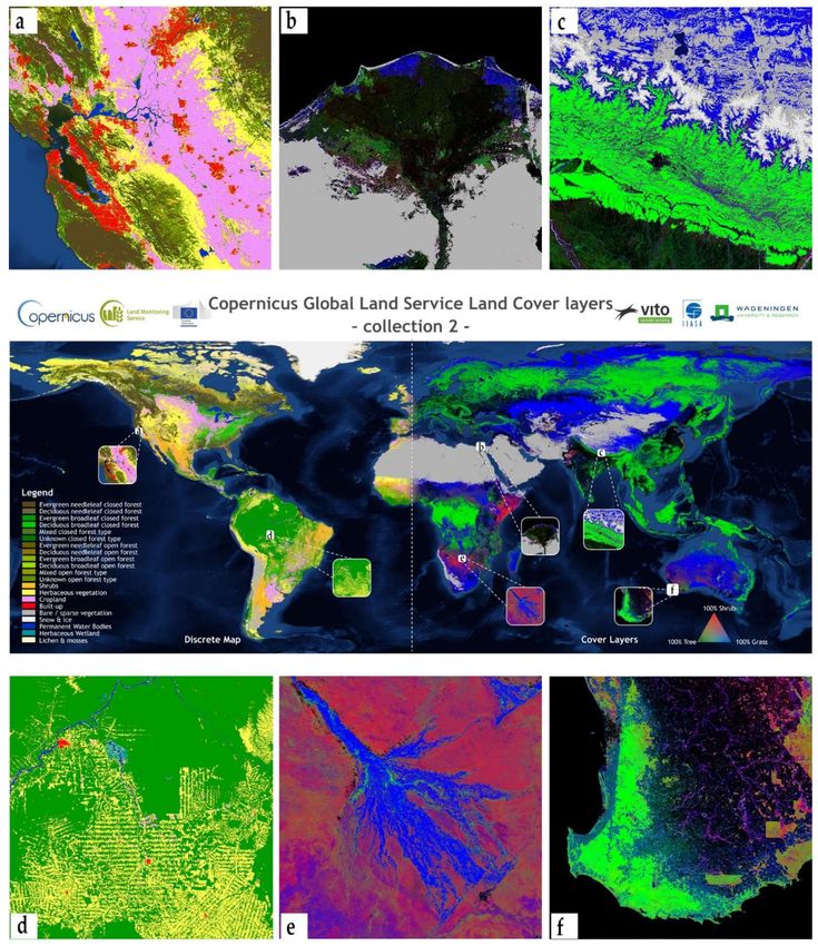
Cover Classification System (LCCS) [38]. Overall, 141,000 unique 100x100 m training locations were
used in the CGLS-LC100 Collection 2 workflow (see Figure 2 for the geographical distribution of the
training data).Remote Sens. 2020, 12, 1044 5 of 14
Figure 2. Training dataset used in the workflow showing the ~141K training locations together with
their sampled land cover class at 100 m. Inlay shows the land cover type distribution in percentage of
the training data. Adapted from [25].
In order to adapt the classification/regressor algorithm to sub-continental and continental patterns,
the classification/regression of the data was carried out per biome, with the biome clusters defined by
the combination of several global ecological layers. In the classification and regression preparation,
the metrics of the training points were analyzed for inter-specific outliers in the pure endmembers,
as well as screened via an all-relevant feature selection approach for the best metrics combinations
(best band selection) for each biome cluster in order to reduce redundant information. Therefore, in a
first step, the metrics are sorted by their separability, and in the second step, reduced via iteratively
removing metrics which are proved by a statistical test to be less relevant than random probes (see [25]
for more details).
2.4. Classification/Regression and Product Generation
The optimized training data set, together with the quality indicator of the input data (DDI
dataset, see Section 2.2) were inputs for the supervised classification algorithms. As the core classifier,
Random Forest (RF) techniques were used. All the generated models were optimized via 5-folded
cross-validation in order to estimate the optimal classifier/regressor parameters.
RF classification was used to produce a hard classification, showing the discrete class for each
pixel, as well as the predicted class probability. This class probability is provided as a quality indicator
layer in the final product. In a second step, the vegetation coverage per pixel was generated via
RF regression, based on the cover fractions collected for all training points, for each class separately.
Moreover, the standard deviation of the applied RF model for each pixel was outputted and added in
the product as additional quality layers. Note that in the final product, the cover fraction layers for
built-up (urban), permanent inland water bodies and seasonal inland water bodies were derived from
the processed ancillary data products.
As a last step, the different classification outputs (discrete map, probability maps as well as the
regression maps), were combined with ancillary data sets to produce the final CGLS-LC100 product
through a set of expert rules. For example, the classes for permanent snow, built-up, and permanent
water were added via rules on the corresponding cover fraction layers. The produced LC map uses a
hierarchical legend based on the UN LCCS. Compatibility with existing global LC products was hereby
taken into account.
2.5. Validation and Comparison
The quality of the CGLS-LC100 product was assessed quantitatively and qualitatively in an
independent validation approach (Figure 1). A detailed description of the methods can be found in theRemote Sens. 2020, 12, 1044 6 of 14
validation report [39]. In short: For the quantitative evaluation, the CGLS-LC100 discrete map was
assessed using an independent validation dataset which includes 21,752 sampling locations across
the globe (2843 to 3616 samples per continent, Table 2 and see Figure 3 for geographical distribution).
The sampling protocol followed the probability sampling scheme [20]. Similar to the training data
collection, validation data was collected on the Geo-Wiki platform, but using an independent branch
from the training data collection [37]. The validation data collection platform was only accessible to
around 30 regional experts with knowledge on satellite-based LC analysis and image interpretation,
who contributed to the validation data collection [39]. More detailed information on the validation
data collection and datasets used for collection is provided in [39,40]. Based on the collected reference
information, fractions of LC types were calculated and used to validate the CGLS-LC100 cover fraction
layers. Specifically, the mean absolute error (MAE) and root mean square error (RMSE) were calculated.
The LC fractions were further translated to a CGLS-LC100 discrete map legend based on the legend
descriptions and used to validate the discrete map. More specifically, a confusion matrix was calculated
based on the mapped and reference LC types. The error matrix was corrected by sample inclusion
probabilities [20].
Figure 3. Validation dataset used in the workflow showing the ~22K validation locations together with
their sampled land cover class at 100 m. Adapted from [39].
A detailed quantitative comparison of the CGLS-LC100 and existing global LC datasets can be
found in the validation report [39]. In summary, for quantitative comparison, Tsendbazar et al. [40]
combined six available reference datasets consisting of around 25,000 points and checked the
correspondence of the resulting dataset with the Globcover 2009, LC-CCI 2010, and MODIS2010
global LC maps and as well as the CGLS-LC100 product. Similarly, the CGLS-LC100 validation
dataset was also used to assess the Globeland30 2010 for comparison with the CGLS-LC100 2015
Collection 2 maps.
All 20 layers forming the CGLS-LC100 Collection 2 product are distributed via several channels
for viewing, on-demand analyses and direct download. See Chapter 4 for more details on the data
access channels.
3. The CGLS-LC100 Product and Accuracy Assessment
The full product specifications (file naming, file format, product content, and characteristics) for
each of the 20 layers in the CGLS-LC100 Collection 2 product [15] can be found in the Product User
Manual (PUM) [41]. This also includes a full description of the Metadata, LC classes, and definitions,
color coding at different classification levels, and found limitations of the dataset.Remote Sens. 2020, 12, 1044 7 of 14
3.1. Global Discrete Map and Cover Fraction Layers
The main product, the CGLS-LC100 discrete map layer (Figure 4), provides a primary LC
scheme at three classification levels, 12 classes at level 1 and up to 23 classes at level 3, with classes
according to the LCCS scheme [38]. Accomplished is the discrete map layer by the CGLS-LC100
forest-type-layer showing the distribution of evergreen needle-leafed and broad-leafed as well as
deciduous needle-leafed and broad-leafed forests.
Figure 4. Overview of the CGLS-LC100 Collection 2 discrete map and cover fraction layers. Center image
shows a collage with the discrete map on the left and a False Color Composite (FCC) showing the cover
fractions layers of shrubland, tree and herbaceous vegetation in the RGB channels. Inlets: (a) discrete
map of the Silicon Valley, US; (b) FCC of the Nile Delta; (c) FCC of Kathmandu; (d) discrete map of
Matogrosso, Brazil; (e) FCC of the Okavango Delta; (f) FCC of the Tierradel elFuego peninsula.
A novelty of the CGLS-LC100 product is the generation of vegetation continuous fields that
provide proportional estimates for vegetation cover for all base classes, i.e., trees, shrubland,
herbaceous vegetation, cropland, moss and lichen, bare ground/sparse vegetation, permanent snow
and ice, built-up and permanent water cover. These nine layers are complemented by a seasonal water
cover fraction layer indicating the area of seasonal water within a pixel. Note: this extra layer is notRemote Sens. 2020, 12, 1044 8 of 14
showing the water occurrence, but if a certain area of a pixel had water coverage up to 11 months in
the year. An overview of these 10 cover fraction layers is shown in Figure 4.
3.2. Quality Indicators
The CGLS-LC100 product delivers, next to the discrete map and cover fraction layers,
eight additional quality layers, which can be used to evaluate pixel-wise the quality of the input EO
data as well as the RF classification and regression quality:
• DDI: The Data Density Indicator indicates the availability of input data from the PROBA-V UTM
ARD+ MC5 archive for 100 m and 300 m resolutions. It is a score between 0 = no input data
available and 100 = best data availability. Overall, 19 single time-series statistics are calculated
and combined via a scoring approach into the DDI. For more details see the ATBD [25].
• Discrete class probability: The probability of the discrete classification indicates the quality of the
discrete classification and is provided as a number between 0 and 100, in steps of 1%. The class
probability is calculated pixel-wise using the RF model and scoring the classification trees within
the RF forest. The higher the probability, the more confident we are that the given class is correct.
• Cover fraction standard deviation: The standard deviation of the percentage cover regression indicates
the quality of the associated cover fraction layer. It is provided as a number between 0 and 100,
in steps of 1%. This indicator is given only for the six classes calculated by the CGLS-LC100
workflow (tree, shrubland, herbaceous vegetation, cropland, moss and lichen, and bare/spare
vegetation). The standard deviation is calculated pixel-wise over the single regression results of
the trees within the RF forest. The lower the standard deviation for a class in a pixel, the higher
the confidence that the result is correct.
3.3. Accuracy Assessment
A full validation report for the CGLS-LC100 Collection 2 product is available for download [39].
It includes a detailed description of the validation sampling design, sampling data collection,
and methods regarding the accuracy assessment including detailed confusion matrixes on global and
continental level for classification levels 1 and 2. We report here only a short summary of the results.
Table 1 shows the confusion matrix for the discrete layer at classification level 1 (base classes)
of the CGLS-LC100 Collection 2 product at a global scale. The overall accuracy is 80.2% +/-0.7%
(confidence intervals at 95% confidence level).
In terms of class-specific accuracies, forest, bare/sparse vegetation, snow/ice, and permanent
water are mapped with very high accuracies (>85%). The class accuracies of herbaceous vegetation,
croplands and built-up are moderate (70%–85%). Built-up class has a higher confusion error with
croplands, forest, and herbaceous vegetation. While herbaceous wetlands, lichen/moss, and shrubs
have lower-class accuracies (Remote Sens. 2020, 12, 1044 9 of 14
~5% and RMSE ~15%. Higher MAE and RMSE (MAE ~9%, RMSE ~17%) are viewable in the tree and
shrubland cover fraction layers. Herbaceous vegetation fraction product has the highest error with
MAE of 17.3% and RMSE of 28.1%. This can be due to difficulty in separating herbaceous vegetation
from other LC types.
Table 1. Confusion matrix for the discrete layer at classification level 1 of the CGLS-LC100 Collection 2
product at a global scale. Adapted from [39].
Herbaceous Vegetation
Bare/sparse Vegetation
Confidence Interval ±
Herbaceous Wetland
Permanent Water
User’s Accuracy
Sample Count
Lichen/moss
Croplands
Snow/ice
Built-up
Shrubs
Forest
Total
Forest 33.1 1.9 1.2 0.6 0.0 0.0 0.0 0.0 0.1 0.1 37.1 38.3 89.4 0.8
Shrubs 1.5 5.8 1.4 0.3 0.0 0.2 0.0 0.0 0.1 0.0 9.3 7.9 62.4 3.1
Herbaceous vegetation 1.2 2.3 13.8 0.6 0.0 0.5 0.0 0.1 0.3 1.0 20.0 19.2 69.2 1.8
Croplands 1.1 0.4 1.6 8.2 0.1 0.0 0.0 0.1 0.1 0.0 11.6 12.6 70.2 2.1
Built-up 0.1 0.0 0.0 0.0 0.5 0.0 0.0 0.0 0.0 0.0 0.6 3.9 77.3 5.7
Bare/sparse vegetation 0.0 0.3 0.8 0.0 0.0 13.5 0.0 0.0 0.0 0.0 14.7 6.5 91.5 1.8
Snow/ice 0.0 0.0 0.0 0.0 0.0 0.1 1.9 0.0 0.0 0.0 2.0 2.4 94.7 3.5
Permanent Water 0.0 0.0 0.0 0.0 0.0 0.1 0.0 2.0 0.0 0.0 2.1 4.0 94.9 2.0
Herbaceous Wetland 0.1 0.1 0.3 0.0 0.0 0.0 0.0 0.1 0.5 0.1 1.1 3.7 46.5 6.3
Lichen/moss 0.0 0.0 0.1 0.0 0.0 0.4 0.0 0.0 0.0 0.9 1.4 1.7 63.9 7.0
Total 37.3 10.9 19.2 9.7 0.7 14.7 2.0 2.3 1.2 2.2 100
Sample count 38.9 9.2 19.4 10.6 3.6 7.3 2.3 4.3 2.6 1.8 100
Producer’s accuracy 88.9 53.4 71.8 83.9 76.1 91.7 98.9 86.8 43.7 42 80.2
Confidence interval ± 0.8 2.8 1.8 2.0 7.6 1.4 0.9 3.2 6.4 5.3 0.7
Table 2. Overall classification accuracy of the discrete layer at classification level 1 of the CGLS-LC100
collection 2 product at continental scale. Adapted from [39].
Number of Samples Overall Accuracy (%) Confidence Intervals ±
Africa 3616 80.1 2.0
Asia 3071 83.3 1.5
Northern Eurasia 2976 79.8 1.6
Europe 3120 80.4 1.6
North America 2843 77.1 1.7
Oceania & Australia 2951 81.9 1.9
South America 3017 79.6 1.5
Table 3. Mean absolute error (MAE) and root mean square error (RMSE) of the fractional cover layers
of the CGLS-LC100 collection 2 product at global scale. Adapted from [39].
Bare/Sparse Vegetation
Herbaceous Vegetation
Lichen/Moss
Snow/Ice
Built-up
Shrub
Crops
Water
Trees
Mean absolute error % (MAE) 9.0 9.4 17.3 5.1 2.9 5.6 0.1 0.8 0.8
Root mean square error % (RMSE) 17.9 17.4 28.1 15.8 15.1 15.6 3.3 5.7 5.9Remote Sens. 2020, 12, 1044 10 of 14
3.4. Quantitative Comparison of CGLS-LC100 and Existing Global LC Datasets
When compared against the combined reference dataset, the CGLS-LC100 2015 Collection 2 map
shows at global scale a higher agreement (by 3%) to the combined reference dataset than the other
tested four global LC maps (Table 4) [39]. Similarly, at a continental scale, the CGLS-LC100 2015
Collection 2 map has consistently higher agreements than the other maps (Table 4) [39]. Only in
South America, MODIS 2010 map has slightly higher accuracy than the CGLS-LC100 2015 Collection
2 map. Please note, that the objective of this comparison is only to indicate the generic quality of
the CGLS-LC100 2015 Collection 2 map as compared to commonly used previous global LC maps.
One must be cautious to compare directly the overall agreement of these maps due to the differences
in the reference years and legend definitions and other differences between the combined reference
dataset and the global LC maps [40]. Anyhow, this result indicates that the CGLS-LC100 2015 Collection
2 map has a comparable, if not better, quality as previous LC maps. Additional comparison studies
verified this indication [20–23].
Table 4. Quantitative comparison of the discrete layer at classification level 1 of the CGLS-LC100
Collection 2 product with other recent global land cover products. Adapted from [39].
CGLS-LC100 2015
Number of Samples Globcover 2009 LC-CCI 2010 MODIS 2010 Globeland30 2010
Collection 2
Global scale 24593 60.0 66.7 69.4 67.3 72.3
Eurasia 10353 65.4 71.1 70.0 72.3 73.6
North America 4686 56.5 67.6 70.1 65.2 73.5
Australia & Oceania 2381 49.7 59.0 69.6 61.8 69.8
Africa 3881 50.8 55.4 62.9 57.2 68.0
South America 3292 66.2 70.0 73.9 70.6 73.1
4. Data Access Channels
To improve the accessibility, the CGLS-LC100 Collection 2 product as well as the product
documentation is distributed via several access channels:
• The LC layers are available for viewing through the Global Land Cover viewer, available at
https://land.copernicus.eu/global/lcviewer. It displays the various LC layers (discrete map,
cover fractions, false-color combinations of cover fractions) on a map, allows us to download
the data in 20x20 degree tiles in the EPSG:4326 projection and reports on LC statistics per
administrative area.
• All products are uploaded on the Zenodo platform for long-term archiving and assigned a concept
DOI as well as a version DOI. The concept DOI will resolve all the time into the newest collection
of the dataset. Moreover, the single layers of the CGLS-LC100 product can be downloaded as
single global files in the ESPG:4326 projection (Table 5).
• All products were ingested into the Google Earth Engine Data Catalog – so now the access through
the Google Earth Engine (GEE) offers on-demand analyses, visualization and data download in
Pseudo-Mercator projection for customized boundary boxes. Search for the term “Copernicus
Global Land Cover Layers: CGLS-LC100 Collection 2” in the GEE Data Catalog.
• The product is also available through the Geo-Wiki engagement platform available at https:
//www.geo-wiki.org/. The user can compare the CGLS-LC100 product with other global and
continental LC products as well as provide feedback or help to collect additional training points
for the next collection of the product.
• More information and documentation about the CGLS-LC100 product is available from the
Copernicus Global Land Service web site at https://land.copernicus.eu/global/products/lc as well
as accessible through the "Copernicus Global Land Service: product documentation" community
on the Zenodo platform at https://zenodo.org/communities/copernicus-land-product-documents/Remote Sens. 2020, 12, 1044 11 of 14
Table 5. Digital Object Identifier information for the CGLS-LC100 collection 2 product.
Attribute Value
Dataset Collection 2
Provided epochs 2015
Dataset version 2.0.2
Concept DOI 10.5281/zenodo.3243508
Version DOI 10.5281/zenodo.3243509
Marcel Buchhorn, Bruno Smets, Luc Bertels, Myroslava Lesiv, Nandin-Erdene Tsendbazar,
Citation Martin Herold, & Steffen Fritz. (2019). Copernicus Global Land Service: Land Cover 100m:
Collection 2: epoch 2015 (Version V2.0.2) [Data set]. Zenodo. DOI: 10.5281/zenodo.3243509
Direct Access http://doi.org/10.5281/zenodo.3243509
Data layers per epoch 20
File Size 63.3 GBytes
5. Conclusions and Outlook
Copernicus currently delivers a dynamic global LC product at 100 m spatial resolution for the
reference year 2015 (CGLS-LC100 Collection 2). Next to a discrete layer, the product also includes
continuous field layers or “fraction maps” for all basic LC classes that provide proportional estimates
for vegetation/ground cover for the LC types. This continuous classification scheme may depict areas
of heterogeneous LC better than the standard classification scheme and, as such, can be tailored for
application use (e.g., forest monitoring, rangeland management, crop monitoring, biodiversity and
conservation, monitoring environment and security in Africa, climate modeling, etc.). Moreover,
the cover fractions layers allow generating LC maps in different legend schemes (i.e., Common
International Classification of Ecosystem Services (CICES) or LCCS). The Minimum Mapping Unit of
100 m and consistent mapping approach allows the usage of the global product on several scales, i.e.,
from regional to global planning.
The highly adaptable CGLS-LC100 mapping approach was already used by other research groups,
e.g., the NatureMap group, a project of the United Nation World Conservation Monitoring Centre,
created a global forest management layer at 100 m with our support [42]; or the Food and Agriculture
Organization of the United Nations (FAO) funded WaPOR (Water Productivity Open-access Portal)
project which generated yearly agriculture maps for Africa starting at 2010 extending the crop class
into irrigated and rainfed agriculture [26].
Our assessments show that the overall accuracy of the discrete layer at classification level 1 of
the CGLS-LC100 Collection 2 product reaches 80.2+/-0.7% at a global and continental scale. The
targeted overall accuracy of 80% has therefore been met. Among the fractional LC layers, snow and
ice, built-up, water and lichen/moss fraction maps show the lowest errors, followed by crops and bare
and sparse vegetation fraction types. On the other hand, fractional herbaceous vegetation cover layer
has the highest error. Our independent quantitative comparisons show that the CGLS-LC100 2015
Collection 2 map has higher accuracy than other available global LC maps.
The third edition of the CGLS-LC100 layers (Collection 3) is currently under preparation covering
the 2015 reference year and annual LC changes from 2016 to 2019 over the entire globe. Firstly, the map
for 2015 will be improved with additional training data (~ 40,000 points) focusing on regions with
lower accuracies. Secondly, for users looking to map land change processes, such as desertification,
de- or re-forestation, urbanization, the impact of major infrastructure developments and so on, it is
important to compare LC maps across different years. The new and additional yearly LC layers
facilitate these processes. Continuity of the service from 2020 onwards is feasible through the use of
Sentinel-1 and Sentinel-2 EO data in the processing line, or going back prior to 2015 through the use of
Landsat EO data.Remote Sens. 2020, 12, 1044 12 of 14
Author Contributions: conceptualization, M.B.; methodology, M.B., L.B. and B.S.; software, M.B., L.B. and
B.S.; validation, N.-E.T., M.L., M.H. and M.B.; formal analysis, M.B., L.B., M.L. and N.-E.T.; investigation, M.B.;
resources, M.B., L.B., B.S. and M.L.; data curation, M.B. and B.S.; writing—original draft preparation, M.B.;
writing—review and editing, M.B., M.L., N.-E.T. and B.S.; visualization, M.B., L.B., M.L. and N.-E.T.; supervision,
B.S. and M.B.; project administration, B.S.; funding acquisition, B.S. All authors have read and agreed to the
published version of the manuscript.
Funding: The product was generated by the Global component of the Land Service of Copernicus, the Earth
Observation programme of the European Commission. The research leading to the current version of the product
has received funding from various European Commission Research and Technical Development programs.
The product is based on PROBA-V data provided by Belgian Science Policy Office (BELSPO) and distributed
by VITO.
Acknowledgments: We would also like to thank all the experts who contributed in developing the training data
set as well to those to who were involved in validation.
Conflicts of Interest: The authors declare no conflict of interest.
References
1. Lambin, E.F.; Meyfroidt, P. Global land use change, economic globalization, and the looming land scarcity.
Proc. Natl. Acad. Sci. USA 2011, 108, 3465–3472. [CrossRef] [PubMed]
2. Tesfaw, A.T.; Pfaff, A.; Kroner, R.E.G.; Qin, S.Y.; Medeiros, R.; Mascia, M.B. Land-use and land-cover change
shape the sustainability and impacts of protected areas. Proc. Natl. Acad. Sci. USA 2018, 115, 2084–2089.
[CrossRef] [PubMed]
3. Cherlet, M.; Hutchinson, C.; Reynolds, J.; Hill, J.; Sommer, S.; von Maltitz, G. World Atlas of Desertification,
3rd ed.; Publication Office of the European Union: Luxembourg, 2018. [CrossRef]
4. Fensholt, R.; Rasmussen, K.; Kaspersen, P.; Huber, S.; Horion, S.; Swinnen, E. Assessing Land
Degradation/Recovery in the African Sahel from Long-Term Earth Observation Based Primary Productivity
and Precipitation Relationships. Remote Sens. 2013, 5, 664–686. [CrossRef]
5. Pedelty, J.; Devadiga, S.; Masuoka, E.; Brown, M.; Pinzon, J.; Tucker, C.; Roy, D.; Ju, J.C.; Vermote, E.; Prince, S.;
et al. Generating a Long-term Land Data Record from the AVHRR and MODIS instruments. Int. Geosci.
Remote Sens. Symp. 2007, 1021–1024. [CrossRef]
6. Ju, J.C.; Masek, J.G. The vegetation greenness trend in Canada and US Alaska from 1984–2012 Landsat data.
Remote Sens. Environ. 2016, 176, 1–16. [CrossRef]
7. Vogelmann, J.E.; Gallant, A.L.; Shi, H.; Zhu, Z. Perspectives on monitoring gradual change across the
continuity of Landsat sensors using time-series data. Remote Sens. Environ. 2016, 185, 258–270. [CrossRef]
8. Congalton, R.G.; Gu, J.Y.; Yadav, K.; Thenkabail, P.; Ozdogan, M. Global Land Cover Mapping: A Review
and Uncertainty Analysis. Remote Sens. 2014, 6, 12070–12093. [CrossRef]
9. Grekousis, G.; Mountrakis, G.; Kavouras, M. An overview of 21 global and 43 regional land-cover mapping
products. Int. J. Remote Sens. 2015, 36, 5309–5335. [CrossRef]
10. Arino, O.; Gross, D.; Ranera, F.; Leroy, M.; Bicheron, P.; Brockman, C.; Defourny, P.; Vancutsem, C.;
Achard, F.; Durieux, L.; et al. GlobCover ESA service for Global land cover from MERIS. Int. Geosci. Remote
Sens. Symp. 2007. [CrossRef]
11. Defourny, P.; Kirches, G.; Brockmann, C.; Boettcher, M.; Peters, M.; Bontemps, S.; Lamarche, C.; Schlerf, M.;
Santoro, M. Land Cover CCI: Product User Guide Version 2. UCL-Geomatics: Ottignies-Louvain-la-Neuve,
Belgium, 2015.
12. Sulla-Menashe, D.; Gray, J.M.; Abercrombie, S.P.; Friedl, M.A. Hierarchical mapping of annual global land
cover 2001 to present: The MODIS Collection 6 Land Cover product. Remote Sens. Environ. 2019, 222, 183–194.
[CrossRef]
13. Gong, P.; Wang, J.; Yu, L.; Zhao, Y.; Zhao, Y.; Liang, L.; Niu, Z.; Huang, X.; Fu, H.; Liu, S.; et al. Finer resolution
observation and monitoring of global land cover: First mapping results with Landsat TM and ETM+ data.
Int. J. Remote Sens. 2013, 34, 2607–2654. [CrossRef]
14. Wulder, M.A.; Coops, N.C.; Roy, D.P.; White, J.C.; Hermosilla, T. Land cover 2.0. Int. J. Remote Sens. 2018,
39, 4254–4284. [CrossRef]
15. Buchhorn, M.; Smets, B.; Bertels, L.; Lesiv, M.; Tsendbazar, N.E.; Herold, M.; Fritz, S. Copernicus Global Land
Service: Land Cover 100m: Epoch 2015: Globe; (Version V2.0.2); Zenodo: Geneve, Switzerland, 2019. [CrossRef]Remote Sens. 2020, 12, 1044 13 of 14
16. Francois, M.; Santandrea, S.; Mellab, K.; Vrancken, D.; Versluys, J. The PROBA-V mission: The space segment.
Int. J. Remote Sens. 2014, 35, 2548–2564. [CrossRef]
17. Dierckx, W.; Sterckx, S.; Benhadj, I.; Livens, S.; Duhoux, G.; Van Achteren, T.; Francois, M.; Mellab, K.;
Saint, G. PROBA-V mission for global vegetation monitoring: Standard products and image quality (vol 35,
pg 2589, 2014). Int. J. Remote Sens. 2016, 37, 1973. [CrossRef]
18. Zhai, Y.G.; Qu, Z.Y.; Hao, L. Land Cover Classification Using Integrated Spectral, Temporal, and Spatial
Features Derived from Remotely Sensed Images. Remote Sens. 2018, 10. [CrossRef]
19. Eberenz, J.; Verbesselt, J.; Herold, M.; Tsendbazar, N.E.; Sabatino, G.; Rivolta, G. Evaluating the Potential of
PROBA-V Satellite Image Time Series for Improving LC Classification in Semi-Arid African Landscapes.
Remote Sens. 2016, 8. [CrossRef]
20. Tsendbazar, N.E.; Herold, M.; de Bruin, S.; Lesiv, M.; Fritz, S.; Van De Kerchove, R.; Buchhorn, M.;
Duerauer, M.; Szantoi, Z.; Pekel, J.F. Developing and applying a multi-purpose land cover validation dataset
for Africa. Remote Sens. Environ. 2018, 219, 298–309. [CrossRef]
21. Nabil, M.; Zhang, M.; Bofana, J.; Wu, B.; Stein, A.; Dong, T.; Zeng, H.; Shang, J. Assessing factors impacting
the spatial discrepancy of remote sensing based cropland products: A case study in Africa. Int. J. Appl. Earth
Obs. Geoinf. 2020, 85, 102010. [CrossRef]
22. Xu, Y.; Yu, L.; Feng, D.; Peng, D.; Li, C.; Huang, X.; Lu, H.; Gong, P. Comparisons of three recent moderate
resolution African land cover datasets: CGLS-LC100, ESA-S2-LC20, and FROM-GLC-Africa30. Int. J.
Remote Sens. 2019, 40, 6185–6202. [CrossRef]
23. Pérez-Hoyos, A.; Udías, A.; Rembold, F. Integrating multiple land cover maps through a multi-criteria
analysis to improve agricultural monitoring in Africa. Int. J. Appl. Earth Obs. Geoinf. 2020, 88, 102064.
[CrossRef]
24. Roy, D.P.; Li, J.; Zhang, H.K.; Yan, L. Best practices for the reprojection and resampling of Sentinel-2 Multi
Spectral Instrument Level 1C data. Remote Sens. Lett. 2016, 7, 1023–1032. [CrossRef]
25. Buchhorn, M.; Bertels, L.; Smets, B.; Lesiv, M.; Tsendbazar, N.E. Copernicus Global Land Service: Land
Cover 100m: Version 2 Globe 2015: Algorithm Theoretical Basis Document; Zenodo: Geneve, Switzerland,
1 January 2019. [CrossRef]
26. FAO. WaPOR, FAO’s Portal to Monitor Water Productivity through Open access of Remotely Sensed Derived
Data. Available online: https//wapor.apps.fao.org/ (accessed on 11 February 2020).
27. Souverijns, N.; Buchhorn, M.; Van De Kerchove, R.; Horion, S.; Brandt, M.; Fensholt, R. 30 years of consistent
land use and land cover changes over the Sahel for the full Landsat era. Remote Sens.. in preparation.
28. Dwyer, J.L.; Roy, D.P.; Sauer, B.; Jenkerson, C.B.; Zhang, H.K.K.; Lymburner, L. Analysis Ready Data:
Enabling Analysis of the Landsat Archive. Remote Sens. 2018, 10. [CrossRef]
29. ESA. Sentinel-2 Tiling Grid Dataset; European Space Agency; Sentinel program, Ed.; European Space Agency,
ESRIN: Rome, Italy, 2018.
30. Roerink, G.J.; Menenti, M.; Verhoef, W. Reconstructing cloudfree NDVI composites using Fourier analysis of
time series. Int. J. Remote Sens. 2000, 21, 1911–1917. [CrossRef]
31. Walker, H.M. Studies in the History of Statistical Method: With Special Reference to Certain Educational
Problems. Williams & Wilkins Co: Baltimore, MD, USA, 1929; p. 24.
32. Verhoef, W. Application of Harmonic Analysis of NDVI Time Series (HANTS). In Fourier Analysis of Temporal
NDVI in the Southern African and American Continents; Azzali, S.M., Ed.; DLO Winand Staring Centre:
Wageningen, The Netherlands, 1996; Volume 108, pp. 19–24.
33. Sedano, F.; Kempeneers, P.; Hurtt, G. A Kalman filter-based method to generate continuous time series of
medium-resolution NDVI images. Remote Sens. 2014, 6, 12381–12408. [CrossRef]
34. Kempeneers, P.; Sedano, F.; Piccard, I.; Eerens, H. Data Assimilation of PROBA-V 100 and 300 m. IEEE J. Sel.
Top. Appl. Earth Obs. Remote Sens. 2016, 9, 3314–3325. [CrossRef]
35. Pekel, J.-F.; Cottam, A.; Gorelick, N.; Belward, A.S. High-resolution mapping of global surface water and its
long-term changes. Nature 2016, 540, 418–422. [CrossRef]
36. Marconcini, M.; Metz-Marconcini, A.; Üreyen, S.; Palacios-Lopez, D.; Hanke, W.; Bachofer, F.; Zeidler, J.;
Esch, T.; Gorelick, N.; Kakarla, A.; et al. Outlining where humans live—The World Settlement Footprint 2015.
arXiv 2019, arXiv:1910.12707.Remote Sens. 2020, 12, 1044 14 of 14
37. Fritz, S.; McCallum, I.; Schill, C.; Perger, C.; See, L.; Schepaschenko, D.; van der Velde, M.; Kraxner, F.;
Obersteiner, M. Geo-Wiki: An online platform for improving global land cover. Environ. Modell. Softw. 2012,
31, 110–123. [CrossRef]
38. Di Gregorio, A.; Food and Agriculture Organization of the United Nations; United Nations Environment
Programme. Land Cover Classification System: Classification Concepts and User Manual: LCCS, Software, 2nd ed.;
Food and Agriculture Organization of the United Nations : Rome, Italy, 2005; 190p.
39. Tsendbazar, N.E.; Herold, M.; Lesiv, M.; Fritz, S. Copernicus Global Land Service: Land Cover 100m: Version 2
Globe 2015: Validation Report; Zenodo: Geneve, Switzerland, 2019. [CrossRef]
40. Tsendbazar, N.E.; de Bruin, S.; Mora, B.; Schouten, L.; Herold, M. Comparative assessment of thematic
accuracy of GLC maps for specific applications using existing reference data. Int. J. Appl. Earth Obs. Geoinf.
2016, 44, 124–135. [CrossRef]
41. Buchhorn, M.; Smets, B.; Bertels, L.; Lesiv, M.; Tsendbazar, N.E.; li, L. Copernicus Global Land Service: Land
Cover 100m: Version 2 Globe 2015: Product User Manual; Zenodo: Geneve, Switzerland, 01 January 2019.
[CrossRef]
42. Nature Map Earth. Nature Map Earth. Available online: https://naturemap.earth/ (accessed on
11 February 2020).
© 2020 by the authors. Licensee MDPI, Basel, Switzerland. This article is an open access
article distributed under the terms and conditions of the Creative Commons Attribution
(CC BY) license (http://creativecommons.org/licenses/by/4.0/).You can also read