Training a convolutional neural network to conserve mass in data assimilation
←
→
Page content transcription
If your browser does not render page correctly, please read the page content below
Nonlin. Processes Geophys., 28, 111–119, 2021
https://doi.org/10.5194/npg-28-111-2021
© Author(s) 2021. This work is distributed under
the Creative Commons Attribution 4.0 License.

Training a convolutional neural network to conserve
mass in data assimilation
Yvonne Ruckstuhl1 , Tijana Janjić1 , and Stephan Rasp2
1 Meteorological   Institute Munich, Ludwig-Maximilians-Universität München, Munich, Germany
2 ClimateAi,   San Francisco, CA, USA

Correspondence: Yvonne Ruckstuhl (yvonne.ruckstuhl@lmu.de)

Received: 2 September 2020 – Discussion started: 25 September 2020
Revised: 15 December 2020 – Accepted: 17 December 2020 – Published: 9 February 2021

Abstract. In previous work, it was shown that the preserva-           and Janjić (2018) that failing to conserve certain quantities
tion of physical properties in the data assimilation framework        like mass, energy and enstrophy can be highly detrimental
can significantly reduce forecast errors. Proposed data assim-        to the estimation of the state. Janjić et al. (2014) proposed a
ilation methods, such as the quadratic programming ensem-             new data assimilation algorithm, the quadratic programming
ble (QPEns) that can impose such constraints on the calcu-            ensemble (QPEns), which replaces the analysis equations of
lation of the analysis, are computationally more expensive,           the EnKF with an ensemble of minimisation problems sub-
severely limiting their application to high-dimensional pre-          ject to physical constraints. Zeng et al. (2017) showed, in an
diction systems as found in Earth sciences. We, therefore,            idealised set-up with a 2 week forecast generated by a 2D
propose using a convolutional neural network (CNN) trained            shallow water model, that error growth is significantly re-
on the difference between the analysis produced by a stan-            duced if the enstrophy is constrained. Similarly, Ruckstuhl
dard ensemble Kalman filter (EnKF) and the QPEns to cor-              and Janjić (2018) illustrated the benefit of constraining the
rect any violations of imposed constraints. In this paper, we         total mass and positivity of precipitation in a simple test case
focus on the conservation of mass and show that, in an ide-           for convective-scale data assimilation. The obstacle that re-
alised set-up, the hybrid of a CNN and the EnKF is capable            mains in applying the QPEns on large systems is the com-
of reducing analysis and background errors to the same level          putational demand of solving the constrained minimisation
as the QPEns.                                                         problems that appear for each ensemble member at each as-
                                                                      similation cycle. For a detailed discussion on the computa-
                                                                      tional costs of the QPEns, we refer to Janjic et al. (2021).
                                                                      In this work, we propose using an artificial neural network
1   Introduction                                                      (NN) to correct the unconstrained solution instead of solving
                                                                      the constrained minimisation problems.
The ensemble Kalman filter (EnKF; Evensen, 1994; Burgers                 NNs are powerful tools to approximate arbitrary nonlinear
et al., 1998; Evensen, 2009) and versions thereof are power-          functions (Nielsen, 2015). A NN learns to recognise patterns
ful data assimilation algorithms that can be applied to prob-         based on examples, rather than being explicitly programmed.
lems that need an estimate of a high-dimensional model state,         An important advantage is that no direct knowledge of the
as in weather forecasting. An important condition for the suc-        function is needed. Instead, a data set consisting of input–
cessful application of the EnKF to a large system is the use of       output pairs is used to train the NN to predict the output cor-
localisation. Any localisation method aims to diminish sam-           responding to a given input. Especially in the fields of image
pling errors caused by the computational limitation of the            recognition and natural language processing, NNs are state of
ensemble size. By doing so, mass conservation, as guaran-             the art and have become a standard tool (LeCun Yann et al.,
teed by a numerical model, is violated during data assimila-          2015). In numerical weather prediction, NNs are not yet fully
tion (Janjić et al., 2014). It was shown in Janjić et al. (2014),   integrated, though interest is rising quickly (Reichstein et al.,
Zeng and Janjić (2016), Zeng et al. (2017) and Ruckstuhl

Published by Copernicus Publications on behalf of the European Geosciences Union & the American Geophysical Union.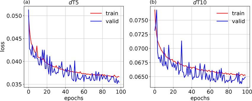
112                                                                         Y. Ruckstuhl et al.: CNN to conserve mass in DA

2019). A recent review of the use of NNs in meteorology can       2     Experiment set-up
be found in McGovern et al. (2019). Explored applications
include (but are not limited to) post-processing of raw model     2.1    Model
output based on observations (McGovern et al., 2017; Rasp
and Lerch, 2021), representing subgrid processes in weather       The modified shallow water model (Würsch and Craig, 2014)
and climate models using high-resolution model simulations        consists of the following equations for the velocity u, rain r
(Krasnopolsky et al., 2013; Rasp et al., 2018; Brenowitz and      and water height level of the fluid h, respectively:
Bretherton, 2019; Yuval and O’Gorman, 2020), combining
                                                                          ∂u ∂ φ + γ 2 r

                                                                  ∂u                                      ∂ 2u
a NN with a knowledge-based model as a hybrid forecast-              +u       +              = βu + Du 2 ,                   (1)
ing approach (Pathak et al., 2018b; Watson, 2019) and re-         ∂t      ∂x          ∂x                  ∂x
placing the numerical weather prediction model altogether         with the following:
(Dueben and Bauer, 2018; Pathak et al., 2018a; Weyn et al.,           (
2020; Scher and Messori, 2019; Rasp et al., 2020; Rasp and              φc if h > hc
                                                                  φ=                                                         (2)
Thuerey, 2020). A general challenge when applying NNs in                gh else,
numerical weather prediction is that the training data often
consist of sparse and noisy data, which NNs are ill equipped      ∂r    ∂r        ∂ 2r
                                                                     +u     = Dr 2 − αr
to handle. Brajard et al. (2020a) and Bocquet et al. (2020)       ∂t    ∂x       ∂x
                                                                      (
proposed using data assimilation in the training process of              ∂u                      ∂u
                                                                        δ , h > hr and                 hc ), rain is produced,
low the extraction of the most information from sparse and        leading to a decrease in the water level and buoyancy. The
noisy observations, as argued in, for example, Brajard et al.     model conserves mass, so the spatial integral over h is con-
(2020a). We aim to produce better results than standard data      stant in time.
assimilation algorithms at minimal additional computational          The 1D model domain, representing 125 km, is discre-
costs by training on data produced by the QPEns.                  tised with n = 250 points, yielding the state vector x =
   We generate our training data by performing twin exper-        [uT hT r T ]T ∈ R750 . The time step is chosen to be 5 s. The
iments with the 1D modified shallow water model (Würsch           forcing βu has a Gaussian shape, with a half-width of four
and Craig, 2014), which was designed to mimic important           grid points and an amplitude of 0.002 m s−1 . This model
properties of convection. These aspects include an acute          was used for testing data assimilation methods in convective-
regime switch when convection is triggered (conditional in-       scale applications in Haslehner et al. (2016) and Ruckstuhl
stability) and a significant time lag between the onset of con-   and Janjić (2018).
vection and its observation. The model is briefly introduced
in Sect. 2.1, followed by the settings of the twin experiments    2.2    Twin experiments
in Sect. 2.2. Section 2.3 provides a report on the generation
of the training data. Since both our input and output are full    The nature run which mimics the true state of the atmosphere
model states, the obvious choice is to train a convolutional      is a model simulation starting from an arbitrary initial state.
neural network (CNN), as the convolution with kernels nat-        The ensemble is chosen to be of a small size with Nens = 10,
urally acts as a form of localisation. The CNN architecture       and, like the nature run, each member starts from an arbitrary
we use for this application is described in Sect. 2.4. The re-    initial state. Observations are assimilated at every dT model
sults are presented in Sect. 3, followed by the conclusion in     time step and are obtained by adding a Gaussian error to the
Sect. 4.                                                          wind u and height h field of the nature run at the correspond-
                                                                  ing time, with a standard deviation of σu = 0.001 m s−1 and

Nonlin. Processes Geophys., 28, 111–119, 2021                                       https://doi.org/10.5194/npg-28-111-2021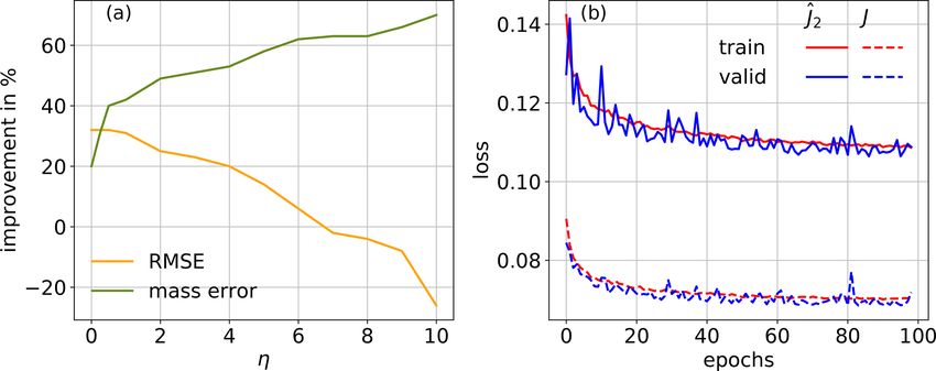
Y. Ruckstuhl et al.: CNN to conserve mass in DA                                                                                         113

σh = 0.01 m, and a log-normal error is added to the rain r
field with the parameters of the underlying normal distri-
bution µ = −8 and σ = 1.5. For all variables, the observa-
tion error is roughly 10 % of the maximum deviation from
the variable mean. To mimic radar data, observations for all
variables are available only on grid points where rain above
a threshold of 0.005 dBZ is measured. A random selection,               Figure 1. Schematic of the generation of the data sets Qbt , Qat and
amounting to 10 % of the remaining grid points of additional            Xat , where MSW stands for modified shallow water model.
wind observations, are assimilated, which represents addi-
tional available data (for example, obtained from aircraft).
   To deal with undersampling, covariance localisation us-
ing the fifth piecewise rational function (Gaspari and Cohn,
1999) is applied with a localisation radius of four grid points.
This corresponds to the localisation radius for which the
EnKF yields minimum analysis root mean squared error
(RMSE) values of the rain variable for an ensemble size of
10. An interior point method is used to solve the quadratic
minimisation problems of the QPEns. The constraints that
are applied are mass conservation, i.e. eT (ha −hb ) = eT δh =          Figure 2. Value of the loss function J averaged over samples for the
0, and positivity of precipitation, i.e. r a = δr + r b ≥ 0. Here,      training (red) and validation (blue) data set as a function of epochs
the superscript b denotes the background and a the analysis,            for dT5 (a) and dT10 (b).
and e is a vector of size n containing only values of one. For
the EnKF, negative values for rain are set to zero if they oc-
cur.                                                                    cles. Both data sets contain the entire ensemble of Nens = 10
                                                                                                     (∗)
   When the assimilation window dT is large enough, the ac-             members, such that (∗)t ∈ RNens ×n×3 , where the last di-
cumulation of mass leads to divergence for the EnKF; that is,           mension represents the three variables (u, h and r), and n
the analysis error is larger than the climatological standard           is the number of grid points.
deviation of the model state. The QPEns converges for all dT,              The output of our training set Ytr ∈ RNens T ×n×3 is sim-
due to its ability to conserve mass. We, therefore, distinguish         ply a reshaped and normalised version of the data set {Qat :
between two cases, namely one where the EnKF converges                  t = 1, 2, . . ., T }. For the input of our training set Xtr , we
(dT = 60; equivalent to 5 min real time) and one where the              choose to use an index vector indicating the position of
EnKF diverges (dT = 120; equivalent to 10 min real time).               the radar observations {It : t = 1, 2, . . ., T }, in addition to the
We refer to Ruckstuhl and Janjić (2018) for a comparison of            unconstrained solutions {Xat : t = 1, 2, . . ., T }, yielding Xtr ∈
the performance of the EnKF and the QPEns as a function                 RNens T ×n×4 , where the index vector It is copied Nens times to
of ensemble size for different localisation radii, assimilation         obtain I∗t ∈ RNens ×n×1 . We include this information because
windows and observation coverage.                                       we know from Ruckstuhl and Janjić (2018) that the strength
                                                                        of the QPEns lies in suppressing spurious convection. Since
2.3   Training data                                                     the radar observations cover only rainy regions, the data set
                                                                        It can help the CNN to distinguish between dry and rainy re-
We aim to produce initial conditions of the same quality as             gions and possibly develop a different regime for each situ-
the ones produced by the QPEns by upgrading the initial con-            ation. We verified that the CNN yields significantly different
ditions produced by the EnKF using a CNN. To that end,                  output when setting all values of It to zero, indicating that
we generate QPEns cycling data {(Qbt , Qat ) : t = 1, 2, . . ., T },    the CNN indeed uses this information. For u and h, the input
where Q stands for QPEns and the superscripts b denote the              and output data set is normalised by subtracting the climato-
background and a the analysis, respectively. In parallel, we            logical mean before dividing by the climatological standard
create the data set {Xat : t = 1, 2, . . ., T }, where Xat is the un-   deviation. For r, we do not subtract the climatological mean
constrained solution calculated from Qbt . See Fig. 1 for a             to maintain positivity.
schematic of the generation process of the data sets. Note                 A validation data set Xvalid and Yvalid is exactly the same
that, by using the background generated from the QPEns                  as the training data set, but a different random seed number is
(Qbt ) in the calculation of both Xat and Qat , we train the CNN        created to monitor the training process. For both the training
only to focus on differences in the minimisation process and            and validation data set, we set T = 4800, which amounts to
not on the possible differences in the background error co-             a total of Nens T = 48 000 training and validation samples,
variances that could have accumulated during cycling. In                respectively.
Sect. 3, we validate this approach by applying the CNN to
the EnKF analysis for 180 subsequent data assimilation cy-

https://doi.org/10.5194/npg-28-111-2021                                             Nonlin. Processes Geophys., 28, 111–119, 2021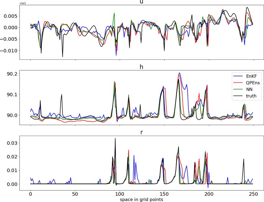
114 Y. Ruckstuhl et al.: CNN to conserve mass in DA
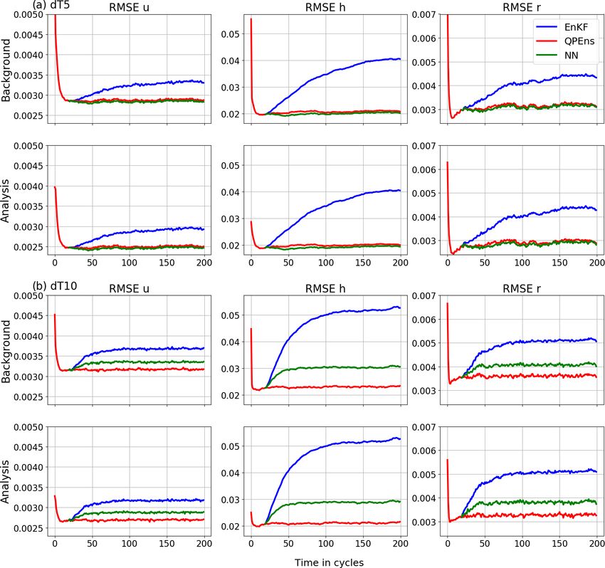
Figure 3. Root mean squared error (RMSE) of the ensemble averaged over 500 experiments of the variables (columns) for the background
(top rows) and analysis (bottom rows) as functions of the assimilation cycles for the EnKF (blue), the QPEns (red) and the CNN (green). The
panels in (a) correspond to dT5 and the panels in (b) to dT10.
2.4 Convolutional neural network (CNN) architecture kernel size is 3. We use a linear activation function for u
and h and the “relu” activation function for r to ensure non-
We choose to use a CNN with four convolutional hidden lay- negativity of rain. We set the batch size to 96 and run 100
ers, consisting of 32 filters each with kernels of size 3, and epochs. Unless stated otherwise, the loss function is defined
the “selu” activation function as follows: as the RMSE over the grid points, averaged over the variables
as follows:
(
x, for x ≥ 0
g(x) = λ1 x
(5) v
λ2 (e − 1) , for x < 0, 1X 3 u
u1 X n 2
p p
J yj (w) = t yj,i,v − yj,i,v ,
where λ1 = 1.05070098 and λ2 = 1.67326324. These values 3 v=1 n i=1
are chosen such that the mean and variance of the inputs
are preserved between two consecutive layers (Klambauer j = 1, . . ., Nens T , (6)
et al., 2017). The output layer is a convolutional layer as p
well, where the number of filters is determined by the de- where yj,i,v and yj,i,v are the prediction and output for
sired shape of the output of the CNN, which is a model state the vth variable of the j th sample at the ith grid point,
(u, h, r) ∈ Rn×3 . The output layer has, therefore, three fil- respectively. The
Adam algorithm is used to minimise
1 PNens T p
ters and the kernel size is again 3. Note that the maximum Nens T j =1 J yj (w) over the weights w of the CNN. The
influence radius of a variable as assumed by the CNN is training is done in the Python library with Keras (Chollet,
(3 − 1)/2 × 5 = 5, where 5 is the number of layers and the 2017).
Nonlin. Processes Geophys., 28, 111–119, 2021 https://doi.org/10.5194/npg-28-111-2021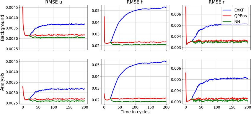
Y. Ruckstuhl et al.: CNN to conserve mass in DA                                                                                       115

                                                                     Figure 5. (a) Relative improvement in the percent of RMSE (or-
                                                                     ange) and mass error (green) towards the output with respect to the
                                                                     input as a function η. (b) Value of the loss function Jˆ (solid) and J
                                                                     (dashed) averaged over samples for the training (red) and validation
                                                                     (blue) data set as function of epochs for dT10η=2 .

Figure 4. Absolute mass error averaged over 500 experiments of          With respect to RMSEs, for dT5 the CNN performs as well
h (a, c) and r (b, d) for the analysis ensemble mean for the EnKF    as the QPEns, despite having learnt during training only 27 %
(blue), QPEns (red) and CNN (green). Panels (a) and (b) correspond   of the difference between the EnKF and QPEns analysis in
to dT5 and panels (c) and (d) to dT10.
                                                                     terms of the loss function. For dT10 the CNN does perform
                                                                     significantly better than the EnKF but clearly remains infe-
                                                                     rior to the QPEns. Given that, in terms of the RMSE over the
3   Results
                                                                     grid points, the CNN for dT10 is slightly better than the one
We assign the name dT5 to the experiment corresponding to            for dT5, we hypothesise that the key to the good performance
a cycling period of 5 min and dT10 to the experiment corre-          of the CNN applied within the data assimilation cycling lies
sponding to a cycling period of 10 min. Figure 2 shows the           in preventing the accumulation of mass in h. When mass ac-
evolution of the loss function averaged over the samples for         cumulates in clear regions, i.e. regions where the nature run
the training and validation data set for dT5 and dT10, respec-       holds h < hc , it has a snowball effect not only on h itself
tively. Table 1 summarises what the CNN has learnt for each          but also on r (see Fig. 4). After all, clouds, and later rain,
variable separately in the two cases. As the training data is        are produced whenever h > hc . For dT5, the CNN does not
normalised, we can conclude from the RMSE of the input               score much better than for dT10 in terms of absolute mass
data with respect to the output data (first row in Table 1) that     error. However, it was able to effectively remove all bias in
the mass constraint on h and the positivity constraints on r         h (with a residual of O(10−5 )), in contrast to the CNN for
impact the solution of the minimisation problem for all vari-        dT10.
ables with the same order of magnitude. Given our choice of             To support this claim, we trained an additional CNN with
loss function, it is not surprising that the relative reduction      the training set corresponding to dT = 10, with a penalty
of the gap between the input and output by the CNN is pro-           term for the mass of h in the loss function as follows:
portional to the size of the gap. By aiming to minimise the                             η X n            n
mean RMSE of all variables, the CNN reduced the violation                 p          p              p
                                                                                                            X
                                                                     Jˆη yj (w) = J yj (w) +       yj,i,2 −     yj,i,2 ,               (7)
of the mass constraint by about 20 % for both experiments.                                   n i=1          i=1
However, for dT5 the reduction in the bias of the height field
is 100 %, while for dT10 it is a mere 30 %.                          where the parameter η is tunable. The larger η, the better
   Next, we are interested in how the CNNs perform when              the mass of h is conserved at the expense of the RMSE (see
applied within the data assimilation cycling. In Fig. 3, we          Fig. 5). We found a good trade-off for η = 2. We refer to this
compare the performance of the EnKF, QPEns and the hybrid            experiment as dT10η=2 . The training process is illustrated in
of CNN and EnKF, where CNN is applied as a correction to             Fig. 5. The mass conservation term comprises about 40 %
the initial conditions computed by the EnKF. To avoid having         of the total loss function Jˆ. Both terms of the loss function
to train a CNN for the spin-up phase where the increments            are decreasing at approximately the same rate throughout the
are larger, we start the data assimilation for the EnKF and          entire training process. Comparing Table 1 with Table 2, we
the CNN from the initial conditions produced by the QPEns            conclude that by adding the penalty term for the mass viola-
at the 20th cycle. The RMSEs shown in Fig. 3 are calculated          tion in the loss function, 7 % of the improvement was lost in
through time against the nature run for both the background          terms of loss function J , but 29 % was gained in the conser-
and the analysis.                                                    vation of mass. Table 3 suggests that the CNN is especially
                                                                     active in clear regions or at the edge of clear regions. Indeed,
                                                                                                                                  dh
                                                                     by far the most significant correlations are with h, r and dx   ,

https://doi.org/10.5194/npg-28-111-2021                                           Nonlin. Processes Geophys., 28, 111–119, 2021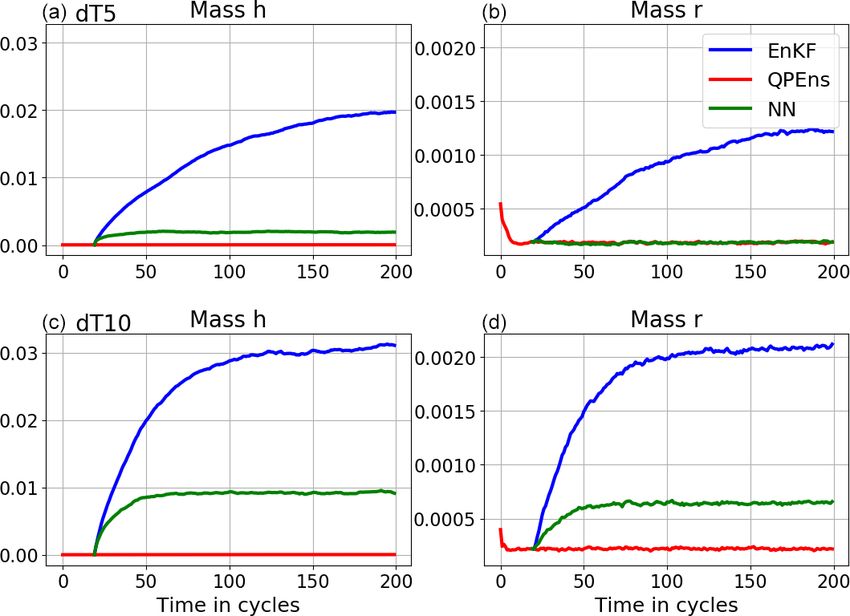
116                                                                                Y. Ruckstuhl et al.: CNN to conserve mass in DA

Table 1. The loss function, the mean RMSE of the variables u, h and r, the absolute mass error divided by the number of grid points n
for h and r, and the bias of h (columns) calculated for the input Xvalid (top row) and the CNN prediction (middle row) with respect to the
output Yvalid for the validation data sets. The last row shows the improvement in the prediction towards the output compared to the input in
percentage. The two sections in the table correspond to dT5 and dT10, respectively.

                Validation               Loss              u               h              r       Mass h        Mass r         Bias h
                Input              4.9 × 10⁻²     4.2 × 10⁻²    4.6 × 10⁻²      5.9 × 10⁻²    1.8 × 10⁻²    4.0 × 10⁻³     1.4 × 10⁻²
      dT5       Prediction         3.6 × 10⁻²     4.1 × 10⁻²    3.9 × 10⁻²      2.7 × 10⁻²    1.4 × 10⁻²    2.9 × 10⁻³             0.0
                Improvement (%)            27             2.8           15              55            22            28            100
                Input              9.6 × 10⁻²     7.9 × 10⁻²    9.0 × 10⁻²      1.2 × 10⁻¹    3.6 × 10⁻²    8.0 × 10⁻³     3.3 × 10⁻²
      dT10      Prediction         6.5 × 10⁻²     7.3 × 10⁻²    6.9 × 10⁻²      5.4 × 10⁻²    2.9 × 10⁻²    7.1 × 10⁻³     2.3 × 10⁻²
                Improvement (%)            32             7.8           24              55            20            11             30

Table 2. The same as Table 1 but for dT10η=2 .

            Validation               Loss              u              h              r        Mass h        Mass r         Bias h
            Input              9.6 × 10⁻²    7.9 × 10⁻²     8.9 × 10⁻²      1.2 × 10⁻¹    3.6 × 10⁻²    7.8 × 10⁻³    3.3 × 10⁻²
            Prediction         7.2 × 10⁻²    7.9 × 10⁻²     8.2 × 10⁻²      5.5 × 10⁻²    1.8 × 10⁻²    7.9 × 10⁻³    8.9 × 10⁻⁴
            Improvement (%)            25            0.7            8.1             53            49            −1           103

Figure 6. The same as Fig. 3 but for dT10η=2 .

                                                                             Figures 6, 7 and 8 show the data assimilation results for
                                                                          dT10η=2 . It is striking that the CNN performs slightly better
                                                                          than the QPEns. Since the CNN only has an influence ra-
                                                                          dius of five grid points and the localisation cut-off radius of
                                                                          the data assimilation is eight grid points, it is possible that
                                                                          the better results of the CNN stem from this shorter influ-
                                                                          ence radius. However, a CNN trained on the same data but
                                                                          with kernel sizes of 5 instead of 3 (leading to an influence
                                                                          radius of 10 grid points) yields similar results as in Figs. 6
Figure 7. The same as Fig. 4 but for dT10η=2 .                            and 7 (not shown). When comparing the input X, output Y
                                                                          and the CNN prediction Yp to the nature run, we found that,
                                                                          for the clear regions, Yp is slightly closer to the nature run in
where the negative sign indicates that the CNN corrects more              terms of RMSE than the QPEns and significantly closer than
in clear regions than in cloudy regions.

Nonlin. Processes Geophys., 28, 111–119, 2021                                                 https://doi.org/10.5194/npg-28-111-2021
Y. Ruckstuhl et al.: CNN to conserve mass in DA 117
Table 3. Correlation coefficient for increments of the output (left column) and the prediction for dT10 (middle column) and dT10η=2 (right
column) with the input (top row) and the gradient of the input (bottom row).
Y−X dT10: Yp − X dT10η=2 : Yp − X
u h r u h r u h r
u −0.1 0.0 0.0 −0.2 0.0 0.0 −0.1 0.1 0.0
X h 0.0 −0.1 −0.1 0.1 −0.2 −0.2 0.2 −0.5 −0.2
r 0.0 −0.1 −0.3 0.1 −0.2 −0.4 0.1 −0.4 −0.4
u −0.1 0.0 0.0 −0.2 0.1 0.0 −0.2 0.1 0.0
dX h −0.2 −0.1 −0.2 −0.4 −0.2 −0.2 −0.4 −0.2 −0.2
dx
r −0.1 −0.1 −0.3 −0.2 −0.2 −0.3 −0.2 −0.1 −0.3
Figure 8. Truth (black) and ensemble mean snapshot for EnKF (blue), QPEns (red) and NN with dT10η=2 (green) before negative rain
values are set to zero for the EnKF.
the EnKF (not shown). We speculate that this is because the the positive influence of the CNN is slightly reduced, but it
QPEns generally lacks mass in regions where there are no still matches the performance of the QPEns. We, therefore,
clouds in both the nature run and the QPEns estimate. The conclude that the success of this approach lies in the abil-
EnKF, on the other hand, overestimates the mass in these re- ity of the CNN to correct for errors of h, especially in clear
gions. This is clearly visible in the snapshot of Fig. 8. As regions.
a result, the true value of h lies between the QPEns and
EnKF estimates. In these regions, it is therefore favourable
that the CNN cannot completely close the gap between the 4 Conclusion
input and output data, as it leads to a better fit to the nature
Geoscience phenomena have several aspects that are differ-
run. We also performed an experiment where h is updated by
ent from standard data science applications, for example,
the CNN, and the other variables remain equal to the EnKF
governing physical laws, noisy observations that are non-
solution, and similar results were obtained as in Figs. 6 and
uniform in space and time from many different sources and
7. When only the clear regions of h are updated by the CNN,
rare, interesting events. This makes the use of NNs particu-
https://doi.org/10.5194/npg-28-111-2021 Nonlin. Processes Geophys., 28, 111–119, 2021118 Y. Ruckstuhl et al.: CNN to conserve mass in DA
larly challenging for convective-scale applications, although References
attempts have been made for predicting rain, hail or torna-
does (McGovern et al., 2019). The approach taken in this Bishop, C. H., Etherton, B. J., and Majumdar, S.: Adaptive sampling
study combines noisy and sparse observations with a dynam- with the ensemble transform Kalman filter. Part I: Theoretical
aspects., Mon. Weather Rev., 129, 420–436, 2001.
ical model using a data assimilation algorithm and, in addi-
Bocquet, M., Brajard, J., Carrassi, A., and Bertino, L.: Bayesian in-
tion, uses a CNN to improve on the conservation of physical ference of chaotic dynamics by merging data assimilation, ma-
laws. In previous work it was shown that, in idealised set-ups, chine learning and expectation-maximization, Foundations of
conserving physical quantities like mass in the data assimi- Data Science, 2, 55–80, https://doi.org/10.3934/fods.2020004,
lation framework using the QPEns can significantly improve 2020.
the estimate of the nature run. Here we show that it is pos- Brajard, J., Carrassi, A., Bocquet, M., and Bertino, L.: Combin-
sible to obtain similar positive results by training a CNN to ing data assimilation and machine learning to emulate a dynam-
conserve mass in a weak sense. By training on the uncon- ical model from sparse and noisy observations: A case study
strained (EnKF)/constrained (QPEns) input/output pair, the with the Lorenz 96 model, J. Comput. Sci.-Neth, 44, 101171,
CNN is able to reduce the mass violation significantly. More- https://doi.org/10.1016/j.jocs.2020.101171, 2020a.
over, we found that adding a penalty term for mass violation Brajard, J., Carrassi, A., Bocquet, M., and Bertino, L.: Combining
data assimilation and machine learning to infer unresolved scale
in the loss function is necessary in one of the two test cases
parametrisation, arXiv [preprint], arXiv:2009.04318, 9 Septem-
to produce data assimilation results that are as good as those ber 2020b.
corresponding to the QPEns. Brenowitz, N. D. and Bretherton, C. S.: Spatially Extended
These encouraging results prompt the question of the fea- Tests of a Neural Network Parametrization Trained by
sibility of this approach being applied to fully complex nu- Coarse-Graining, J. Adv. Model. Earth Sy., 11, 2728–2744,
merical weather prediction systems. The challenge here lies https://doi.org/10.1029/2019MS001711, 2019.
in the generation of the training data. First, the effectiveness Burgers, G., van Leeuwen, P. J., and Evensen, G.: Analysis Scheme
of conserving different quantities has to be verified in a non- in the Ensemble Kalman Filter., Mon. Weather Rev., 126, 1719–
idealised numerical weather prediction framework, where the 1724, 1998.
quantities to be conserved may not be known and may not Chollet, F.: Deep Learning with Python, Manning Publications
be exactly conserved within the numerical weather predic- Company, Greenwich, CT, USA, 2017.
Cintra, R. S. C. and de Campos Velho, H. F.: Data Assimilation by
tion model (Dubinkina, 2018). A second consideration is the
Artificial Neural Networks for an Atmospheric General Circu-
computational cost. Advances are made in this regard (Jan-
lation Model: Conventional Observation, CoRR, abs/1407.4360,
jic et al., 2021) but effort and collaboration with optimisation arXiv [preprint], arXiv:1407.4360, 16 July 2014.
experts are still required to allow the generation of a reason- Dubinkina, S.: Relevance of conservative numerical schemes for an
ably large training data set. Ensemble Kalman Filter, Q. J. Roy. Meteor. Soc., 144, 468–477,
https://doi.org/10.1002/qj.3219, 2018.
Dueben, P. D. and Bauer, P.: Challenges and design choices
Code and data availability. The provided source code for global weather and climate models based on ma-
(https://doi.org/10.5281/zenodo.4354602, Ruckstuhl et al., chine learning, Geosci. Model Dev., 11, 3999–4009,
2020) includes the necessary scripts to produce the data. https://doi.org/10.5194/gmd-11-3999-2018, 2018.
Evensen, G.: Sequential data assimilation with a nonliear quasi-
gepstrophic model using Monte Carlo methods to forecast error
Author contributions. YR set up and performed the experiments statistics., J. Geophys. Res., 99, 10143–10162, 1994.
and prepared the paper with contributions from all coauthors. SR Evensen, G.: Data Assimilation: The Ensemble Kalman Filter,
set up the code for the CNN. TJ contributed to the scientific design Springer-Verlag Berlin Heidelberg, Germany, 2009.
of the study and the analysis of the numerical results. Farchi, A., Laloyaux, P., Bonavita, M., and Bocquet, M.: Using ma-
chine learning to correct model error in data assimilation and
forecast applications, arXiv [preprint], arXiv:2010.12605, 23 Oc-
Competing interests. The authors declare that they have no conflict tober 2020.
of interest. Gaspari, G. and Cohn, S. E.: Construction of correlation functions
in two and three dimensions, Q. J. Roy. Meteor. Soc., 125, 723–
757, 1999.
Haslehner, M., Janjic, T., and Craig, G. C.: Testing particle fil-
Financial support. This research has been supported by the Ger-
ters on simple convective-scale models. Part 2: A modified
man Research Foundation (DFG; subproject B6 of the Transre-
shallow-water model, Q. J. Roy. Meteor. Soc., 142, 1628–1646,
gional Collaborative Research Project SFB/TRR 165, “Waves to
https://doi.org/10.1002/qj.2757, 2016.
Weather” and grant no. JA 1077/4-1).
Hunt, B. R., Kostelich, E. J., and Szunyogh, I.: Efficient Data As-
similation for Spatiotemporal Chaos: A local Ensemble Trans-
form Kalman filter., Physica, 230, 112–126, 2007.
Review statement. This paper was edited by Alberto Carrassi and Janjić, T., McLaughlin, D., Cohn, S. E., and Verlaan, M.: Conserva-
reviewed by Marc Bocquet and Svetlana Dubinkina. tion of mass and preservation of positivity with ensemble-type
Nonlin. Processes Geophys., 28, 111–119, 2021 https://doi.org/10.5194/npg-28-111-2021Y. Ruckstuhl et al.: CNN to conserve mass in DA 119 Kalman filter algorithms, Mon. Weather Rev., 142, 755–773, Rasp, S. and Thuerey, N.: Data-driven medium-range weather pre- 2014. diction with a Resnet pretrained on climate simulations: A new Janjic, T., Ruckstuhl, Y., and Toint, P. L.: A data assimilation algo- model for WeatherBench, arXiv [preprint], arXiv:2008.08626, rithm for predicting rain, Q. J. Roy. Meteor. Soc., accepted with 19 August 2020. minor revisions, 2021. Rasp, S., Pritchard, M. S., and Gentine, P.: Deep learning to repre- Jin, J., Lin, H. X., Segers, A., Xie, Y., and Heemink, A.: Machine sent subgrid processes in climate models, P. Natl. Acad. Sci., 115, learning for observation bias correction with application to dust 9684–9689, https://doi.org/10.1073/pnas.1810286115, 2018. storm data assimilation, Atmos. Chem. Phys., 19, 10009–10026, Rasp, S., Dueben, P. D., Scher, S., Weyn, J. A., Mouatadid, https://doi.org/10.5194/acp-19-10009-2019, 2019. S., and Thuerey, N.: WeatherBench: A benchmark dataset for Klambauer, G., Unterthiner, T., Mayr, A., and Hochreiter, data-driven weather forecasting, J. Adv. Model. Earth Syst., S.: Self-Normalizing Neural Networks, arXiv [preprint], 12, e2020MS002203, https://doi.org/10.1029/2020MS002203, arXiv:1706.02515, 8 June 2017. 2020. Krasnopolsky, V. M., Fox-Rabinovitz, M. S., and Belochitski, Reichstein, M., Camps-Valls, G., and Stevens, B.: Deep learn- A. A.: Using ensemble of neural networks to learn stochas- ing and process understanding for data-driven Earth system tic convection parameterizations for climate and numerical science, Nature, 566, 195–204, https://doi.org/10.1038/s41586- weather prediction models from data simulated by a cloud 019-0912-1, 2019. resolving model, Adv. Artif. Neural Syst., 2013, 485913, Ruckstuhl, Y. and Janjić, T.: Parameter and state estimation https://doi.org/10.1155/2013/485913, 2013. with ensemble Kalman filter based algorithms for convective- LeCun Yann, Bengio Yoshua, and Hinton Geoffrey: Deep learn- scale applications, Q. J. Roy. Meteor. Soc, 144, 826–841, ing, Nature, 521, 436–444, https://doi.org/10.1038/nature14539, https://doi.org/10.1002/qj.3257, 2018. 2015. Ruckstuhl, Y., Rasp, S., Würsch, M., and Janjic, T.: McGovern, A., Elmore, K. L., Gagne, David John, I., Haupt, S. E., CNN to conserve mass in data assimilation, Zeonodo, Karstens, C. D., Lagerquist, R., Smith, T., and Williams, J. K.: https://doi.org/10.5281/zenodo.4354602, 2020. Using Artificial Intelligence to Improve Real-Time Decision- Scher, S. and Messori, G.: Weather and climate forecasting with Making for High-Impact Weather, B. Am. Meteor. Soc., 98, neural networks: using general circulation models (GCMs) with 2073–2090, https://doi.org/10.1175/BAMS-D-16-0123.1, 2017. different complexity as a study ground, Geosci. Model Dev., 12, McGovern, A., Lagerquist, R., John Gagne, David, I., Jergensen, 2797–2809, https://doi.org/10.5194/gmd-12-2797-2019, 2019. G. E., Elmore, K. L., Homeyer, C. R., and Smith, T.: Making the Watson, P. A. G.: Applying Machine Learning to Improve Sim- Black Box More Transparent: Understanding the Physical Impli- ulations of a Chaotic Dynamical System Using Empirical Er- cations of Machine Learning, B. Am. Meteor. Soc., 100, 2175– ror Correction, J. Adv. Model. Earth Sy., 11, 1402–1417, 2199, https://doi.org/10.1175/BAMS-D-18-0195.1, 2019. https://doi.org/10.1029/2018MS001597, 2019. Moosavi, A., Attia, A., and Sandu, A.: Tuning Covariance Localiza- Weyn, J. A., Durran, D. R., and Caruana, R.: Improving data- tion Using Machine Learning, in: Computational Science, ICCS driven global weather prediction using deep convolutional neu- 2019. Lecture Notes in Computer Science, vol. 11539, Springer, ral networks on a cubed sphere, J. Adv. Model. Earth Syst., Cham., https://doi.org/10.1007/978-3-030-22747-0_16, 2019. 12, e2020MS002109, https://doi.org/10.1029/2020MS002109, Nielsen, M. A.: Neural networks and deep learning, Determi- 2020. nation press, available at: https://books.google.ch/books?id= Würsch, M. and Craig, G. C.: A simple dynamical model of cumu- STDBswEACAAJ (last access: 2 February 2021), 2015. lus convection for data assimilation research, Meteorol. Z., 23, Pathak, J., Hunt, B., Girvan, M., Lu, Z., and Ott, E.: Model- 483–490, 2014. Free Prediction of Large Spatiotemporally Chaotic Systems Yuval, J. and O’Gorman, P. A.: Stable machine-learning parameter- from Data: A Reservoir Computing Approach, Phys. Rev. Lett., ization of subgrid processes for climate modeling at a range of 120, 024102, https://doi.org/10.1103/PhysRevLett.120.024102, resolutions, Nat. Commun., 11, 1–10, 2020. 2018a. Zeng, Y. and Janjić, T.: Study of conservation laws with the Local Pathak, J., Wikner, A., Fussell, R., Chandra, S., Hunt, B. R., Girvan, Ensemble Transform Kalman Filter, Q. J. Roy. Meteor. Soc., 142, M., and Ott, E.: Hybrid forecasting of chaotic processes: Using 2359–2372, https://doi.org/10.1002/qj.2829, 2016. machine learning in conjunction with a knowledge-based model, Zeng, Y., Janjić, T., Ruckstuhl, Y., and Verlaan, M.: Ensemble- Chaos: An Interdisciplinary J. Nonlinear Sci., 28, 041101, type Kalman filter algorithm conserving mass, total energy https://doi.org/10.1063/1.5028373, 2018b. and enstrophy, Q. J. Roy. Meteor. Soc., 143, 2902–2914, Rasp, S. and Lerch, S.: Neural networks for post-processing en- https://doi.org/10.1002/qj.3142, 2017. semble weather forecasts, Mon. Weather Rev., 146, 3885–3900, https://doi.org/10.1175/MWR-D-18-0187.1, 2021. https://doi.org/10.5194/npg-28-111-2021 Nonlin. Processes Geophys., 28, 111–119, 2021
You can also read