MOFA: MODULAR FACTORIAL DESIGN FOR HYPER-PARAMETER OPTIMIZATION
←
→
Page content transcription
If your browser does not render page correctly, please read the page content below
Under review as a conference paper at ICLR 2021

MOFA: M ODULAR FACTORIAL D ESIGN                                             FOR      H YPER -
PARAMETER O PTIMIZATION

 Anonymous authors
 Paper under double-blind review

                                           A BSTRACT
         Automated hyperparameter optimization (HPO) has shown great power in many
         machine learning applications. While existing methods suffer from model selec-
         tion, parallelism, or sample efficiency, this paper presents a new HPO method,
         MOdular FActorial Design (MOFA), to address these issues simultaneously. The
         major idea is to use techniques from Experimental Designs to improve sample
         efficiency of model-free methods. Particularly, MOFA runs with four modules
         in each iteration: (1) an Orthogonal Latin Hypercube (OLH)-based sampler pre-
         serving both univariate projection uniformity and orthogonality; (2) a highly par-
         allelized evaluator; (3) a transformer to collapse the OLH performance table into
         a specified Fractional Factorial Design–Orthogonal Array (OA); (4) an analyzer
         including Factorial Performance Analysis and Factorial Importance Analysis to
         narrow down the search space. We theoretically and empirically show that MOFA
         has great advantages over existing model-based and model-free methods.

1   I NTRODUCTION
Modern machine learning techniques, especially deep learning, have achieved excellent perfor-
mances in computer vision (Szegedy et al., 2016; Redmon et al., 2016; He et al., 2017), natural
language processing (Vaswani et al., 2017; Devlin et al., 2018) and speech recognition (Zhang
et al., 2017; Lee et al., 2020). However, the performances of these models highly depend on the
configurations of their hyperparameters (Feurer & Hutter, 2019). For example, the performance of
the deep neural networks may fluctuate dramatically under different neural architectures (Liu et al.,
2018b) (Liu et al., 2018a). Different data augmentation policies can lead to different experimental
results for an image recognition task (Cubuk et al., 2019). Heuristic tuning by using prior knowledge
of an expert is a possible solution but only works in simple settings with few hyperparameters.
To save the resource of expert’s experience, automated hyperparameter optimization (HPO) (Yao
et al., 2018; Feurer et al., 2015) is proposed to search for optimum hyperparameters such as learning
rate, batch size and layers (Yu & Zhu, 2020). Currently, there are two lines of works focusing
on HPO (see Appendix A for a more detailed review). (1) Model-based methods: model-based
HPO methods such as Bayesian Optimization (Mockus et al., 1978) optimizing hyperparameters
by learning a surrogate model (e.g. Gaussian process). Although there are many more advantaged
approaches such as TPE (Bergstra et al., 2011), SMAC (Hutter et al., 2011), Hyperband (Li et al.,
2017), BOHB (Falkner et al., 2018) and Reinforcement Learning (RL) (Zoph & Le, 2016), these
methods are highly depending on the parametric model and suffer from parallelism issue due to
their sequential learning-based nature. (2) Model-free methods: model-free methods (e.g. Random
Search) have no dependency on any parametric model, and they can run in a fully parallel fashion
since different configurations run individually without the influence of time sequence (Yu & Zhu,
2020). Nevertheless, Random Search’s sample-efficiency is not enough and time-consuming to get
a global optimal result. For improving sample-efficiency, the field of Experimental Design (Wu &
Hamada, 2011) has made much progress. In an experiment, we deliberately change one or more
factors to observe the change of performance. Experimental Design is a procedure for planning
efficient experiments so that the data obtained can be analyzed with proper methods to yield valid
and objective conclusions. Usually, it can reduce many runs of an experiment to achieve the same
accuracy. There are some HPO applications of Experimental Design, such as Latin Hypercubes
(Brockhoff et al., 2015; Konen et al., 2011; Jones et al., 1998) and Orthogonal Arrays (OAs) (Zhang
et al., 2019). However, they just used these designs directly without matched analysis inference.

                                                 1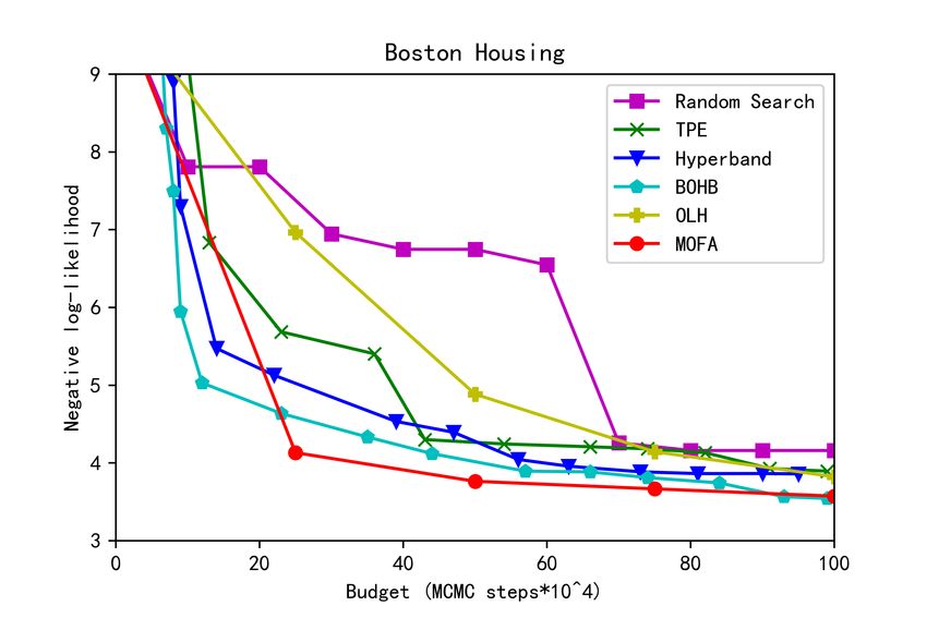
Under review as a conference paper at ICLR 2021

Different from previous model-based and model-free HPO methods, this paper presents a new
model-free HPO method, MOdular FActorial Design (MOFA), which is a multi-module process with
factorial analysis for combinations of multiple factors at multiple levels. MOFA runs iteratively with
four modules in each iteration: Firstly, we propose an Orthogonal Latin Hypercube (OLH)-based
sampler that preserves both univariate (one-dimensional) projection uniformity and orthogonality
to sample hyperparameter configurations; Secondly, a highly-parallelized evaluator is adopted for
configurations evaluation; Thirdly, a transformer is used to collapse the OLH performance table into
a specified Fractional Factorial Design–OA; Finally, an analyzer, including Factorial Performance
Analysis and Factorial Importance Analysis is conducted to narrow down the search space and select
significant hyperparameters for iterative optimization. The intuition is that: (1) the univariate pro-
jection uniformity of OLH makes it explores the search space more sufficient; (2) the orthogonality
of OLH eliminates the interaction between factors to evaluate their main effects, thus is suitable
for factorial analysis, and (3) OLH supports continuous, discrete and mixed search space while OA
only works on discrete space. Theoretical analysis together with empirical results shows that MOFA
outperforms existing model-based and model-free HPO methods.
To summarize, the main contributions in this paper are threefold: (1) We propose a new HPO
method-MOFA, which has the advantages of model-free, parallelizable and sample efficient simul-
taneously. (2) We propose Factorial Performance Analysis and Factorial Importance Analysis to
narrow down the search space and select influential hyperparameters for iterative optimization. (3)
We present a theoretical analysis of the advantages of OLH towards accuracy and robustness. Em-
pirical results further demonstrate that our method outperforms baseline work.

2   P RELIMINARIES
Latin Hypercubes. A Latin Hypercube (McKay et al., 1979) is an N × d table for an N -run
experiment with d factors, which is based on the Latin Square, where there is only one point in
each row and column from a gridded space. A Latin Hypercube is the generalization of the Latin
Square to an arbitrary number of dimensions, whereby each sample is the only one in each axis-
aligned hyper-plane containing it. Fig. 1c (left) shows an example of a Latin Hypercube of nine runs
and three factors. A Latin Hypercube has the property of univariate or one-dimensional projection
uniformity that by projecting an N -point design on to any factor, we will get N different levels for
that factor (Tang, 1993). This property makes Latin Hypercubes drastically reduces the number of
experimental runs necessary to achieve a reasonably accurate result (Bergstra & Bengio, 2012).
Orthogonal Arrays. A Full Factorial Design for HPO tries all possible hyperparameter
configurations–which is generally not acceptable due to combinatorial explosion. To reduce the
number of experimental runs, Fractional Factorial Design carefully selects a subset (a fraction) of
all experimental runs (Mukerjee & Wu, 2007). OA design is a type of general Fractional Factorial
Design. An OA is an N × d table, and each factor has l levels. For any t columns, the different level
combinations appear with equal frequency (t-dimensional orthogonality). The number t is called
the strength of the OA. Based on the definition of OA, a Latin Hypercube is a special OA of strength
one. Moreover, an example of OA of strength two, nine runs, three factors and three levels is shown
in Fig. 1c (right). The orthogonality in OA ensures that each factor’s main effect can be evaluated
without the influence of interaction with other factors.
Orthogonal Latin Hypercubes. A randomly generated Latin Hypercube may be quite structured:
the design may not have good univariate projection uniformity or the different factors are highly
correlated (Joseph & Hung, 2008). To address these issues, several optimal criteria such as mini-
mum correlation Tang (1998) and maximin distance (Franco, 2008) are proposed. Considering the
property of OA, we use OA to construct Latin Hypercubes (OLH) (Tang, 1993) (see Appendix B.3).
Compared with non-orthogonal Latin Hypercubes, OLH preserves both univariate projection unifor-
mity and t-dimensional orthogonality, making it more suitable for factorial analysis. Besides, OLH
supports both continual and discrete search space while OA only supports discrete space.

3   M ODULAR FACTORIAL D ESIGN FOR H YPERPARAMETER O PTIMIZATION
Fig. 1 shows an overview of MOFA. Firstly, an initial search space (continual, discrete, or mixed)
is designed by humans with prior knowledge. Then, MOFA runs iteratively with four modules in

                                                  2
Under review as a conference paper at ICLR 2021

Figure 1: The overview of MOFA. MOFA consists of four individual modules. (a) an OLH-based
sampler for hyperparameter sampling; (b) a paralleled evaluator; (c) a transformer collapsing OLH
performance table into OA. (d) an analyzer to narrow down the search space.

each iteration. In the sampler (Fig. 1a), we construct an OLH preserving both univariate projec-
tion uniformity and orthogonality to sample the hyperparameter configurations. In the evaluator
(Fig. 1b), the sampled hyperparameter configurations are evaluated in parallel. In the transformer
(Fig. 1c), an OLH performance table is built based on the evaluated results and collapsed into a Frac-
tional Factorial Design–OA. In the analyzer (Fig. 1d), Factorial Performance Analysis and Factorial
Importance Analysis are conducted to narrow down the search space and select influential hyperpa-
rameters. Subsequently, a new hyperparameter search space (ROI) is generated and reshaped for a
subsequent search. The termination conditions and the strategies for final hyperparameter selection
are described in Sec. 3.5. The complete pseudocode of this algorithm is presented in Appendix B.1.

3.1   S AMPLER : H YPERPARAMETER S AMPLING WITH OLH

In the sampler (Fig. 1a), we first normalize the search space for each (discrete or continuous) hyper-
parameter into [0, 1] so that each hyperparameter is located in the same sampling space. Secondly,
we build an OLH that preserves both one-dimensional projection uniformity and orthogonality to
sample hyperparameter configurations. The OLH-based sampler has three advantages: (1) OLH
guarantees the one-dimensional projection uniformity, making it explores the search space more

                                                  3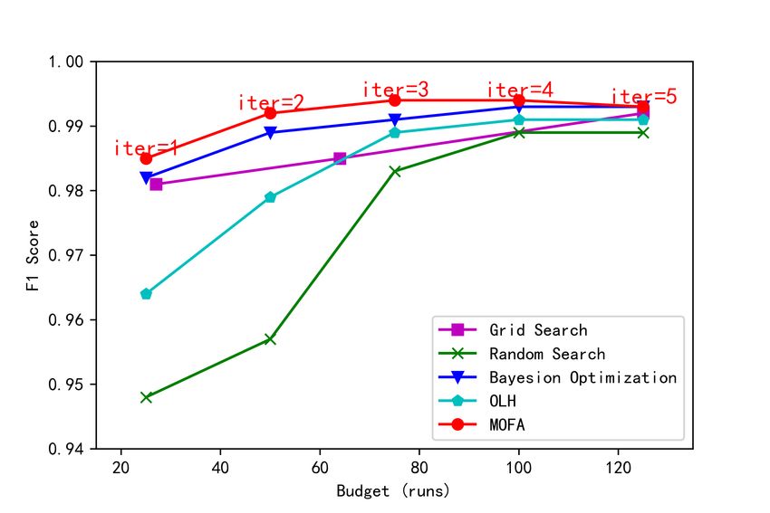
Under review as a conference paper at ICLR 2021

sufficient; (2) the orthogonality of OLH eliminates the interaction between factors to evaluate their
main effects, thus is suitable for factorial analysis (see Sec. 3.4); (3) OLH supports continual, dis-
crete and mixed search space while OA only works on discrete space. For OLH construction, we use
a standard method proposed by Tang (1993) and an open-source R implementation 1 . The details of
OLH construction are beyond the scope of our method, so we describe it in Appendix B.3.

3.2      E VALUATOR : PARALLEL H YPERPARAMETERS E VALUATION

Different from model-based methods that learn a parametric model and update it based on previous
experiences, the hyperparameter configurations sampled by OLH are completely independent with-
out the influence of the time sequence, so they can be evaluated fully in parallel. We do not do extra
experiments in a specific parallel platform, but theoretically analysis the parallelization in Sec. 4.4.

3.3      T RANSFORMER : T RANSFORMING OLH INTO OA

After evaluating all of the sampled hyperparameter configurations, we build an OLH performance
table to store all the hyperparameter settings and evaluation results as Fig. 1c (left) showing. To
facilitate Factorial Analysis that requires discrete levels as input, we transform the continual levels
in the OLH performance table into discrete levels with range collapsing. The method is straightfor-
ward: we group the continual levels in each column of OLH into R ordered ranges based on their
values (highlighted with colors). As the OLH is orthogonal, the collapsed OLH will be an OA of N
runs and N/R levels, where N is the total runs of OLH and R is the range size designed by humans.

3.4      A NALYZER : FACTORIAL A NALYSIS

In the analyzer (Fig. 1d), we aim at narrowing down the search space for subsequent optimization
by analyzing the evaluated experiments in the current iteration. Appendix B.2 shows the full pseu-
docode of the analyzer, where there are following two basic sub-modules.
Factorial Performance Analysis: Based on the collapsed OA, we calculate the marginal mean
performance of each range for each factor and then pick the range with the best mean performance
as the range to be searched. For example, in Fig. 1c, the best mean performance of factor LR is
ranged 0.819, therefore the corresponding range 1 is selected as the best range of LR. Similarly,
range 1 and range 2 are selected as the best range of factor LAM and Units respectively. Since OA
satisfies orthogonality, the marginal mean performance can be seen as an approximate of the overall
performance of each range for each factor, even when some factors are highly correlated.
Factorial Importance Analysis: To further reduce the search space, we analyze the importance
of each factor and freeze the unimportant factors. We use the marginal variance-ratio to measure
the importance of each factor, as the marginal variance can reflect the stability of the factors. For
example, if a factor is not stable, it indicates that the factor needs to be explored more. Conversely,
for a stable or unimportant factor (the importance is less than a specified threshold of β), we directly
freeze it to the current best level (here, we use the median of the current search range as the best
level). For example, the importance (marginal variance ratio) of factor LR, LAM and Units in the
current best range are 0.55, 0.37 and 0.08 respectively, and the importance of Units is less than the
specified threshold 0.1, so we freeze the Units as 0.5 (median of current best range).

3.5      F INAL H YPERPARAMETER S ELECTION

The termination condition can be designed case-by-case, here we stop iterating when the accuracy
of our model reaches a specified threshold or the budget is exhausted, or all factors are frozen. When
the iteration end, two strategies are used to select the final hyperparameter configuration. (1) Greedy
Strategy: we choose the hyperparameter configuration with the best performance among all of the
evaluated experiments as the final hyperparameter selection. The final configuration selected by this
strategy may not be in the last iteration, so it possesses some robustness to over-fitting. (2) Mean
Strategy: we do a Factorial Performance Analysis for the hyperparameters that have not yet been
determined and use the median level of the search range with the largest marginal mean performance
   1
       https://github.com/bertcarnell/lhs

                                                   4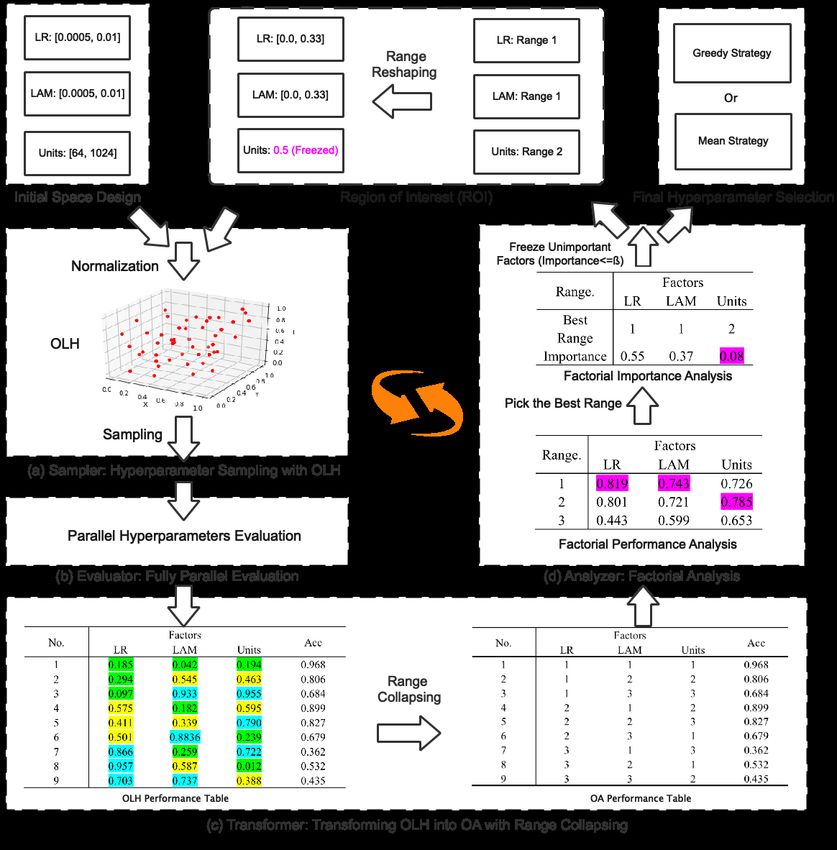
Under review as a conference paper at ICLR 2021

as the final configuration. The hyperparameters selected by this strategy may be better than Greedy
Strategy but may also suffer from over-fitting. To take advantage of both strategies, we combine
these two strategies and pick the best hyperparameter configuration among these strategies.

3.6   H YPER -H YPERPARAMETERS S ETTINGS

One potential disadvantage of MOFA is that there are still some hyperparameters that must be
tuned by humans such as range size R and the importance threshold β, which are called hyper-
hyperparameters. We observed that most of the hyper-hyperparameters in MOFA can be seen as a
trade-off between budgets and accuracy, so it can be determined by users and analyzed case-by-case.
Here we present some experience on how to set good hyper-hyperparameters.
Range Size. One important hyper-hyperparameter
                                      √             is the range size R. R should be carefully de-
signed and must not be larger than b N c, where N is the sampling size (the number of rows of
OLH). Otherwise, the uniformity of sample distribution between range groups will not be satis-
fied when conducting the analysis. To ensure that there are enough samples in each range group
after grouping, the number of samples in each group should not less than the number of groups.
           p bN/Rc >= R. Therefore, the best trade-off between these two restrictions is to
In other word,
set R = b N/Qc, where Q is a small integer. We observed that the best Q was 1 and simply
increasing Q did not significantly change the performance but increased the sample sizes.
Importance Threshold. Importance threshold β is used to evaluate the necessity for subsequent
search of hyperparameters. One most conservative and straightforward method is to set β = 0, in
which case all hyperparameters will be searched with the maximum number of iterations. We do not
do that since different hyperparameters have different effects on the performance, a well designed
β can be used to reduce the risk of over-fitting since searching for unimportant hyperparameters
will lead to a sub-optimal solution. To relieve their influence on HPO tasks, we add a constraint
0 < β < 1/F ∗ P , where F is the number of factors, P is a small integer, we empirically set P = 3.

3.7   T HEORETICAL A NALYSIS

In this section, we analyze the theoretical properties of MOFA in two aspects, improving the accu-
racy by reducing the error bound of the estimator and the robustness by variance reduction.
Accuracy. For factorial analysis, if we use Random Search to draw X1 , . . . , XN independently from
                                          PN
a uniform distribution and use Ȳ = N −1 i=1 f (Xi ) as an estimate of its effect, this estimator will
approach the expectation Ef (X). In this case, one can use the Koksma-Hlawka inequality (Koksma,
1942; Hlawka, 1971; Aistleitner et al., 2015), |Ef (X)− Ȳ | ≤ V (f )·D∗ (X1 , . . . , XN ), where V (f )
is the variation in the sense of Hardy and Krause and D∗ is the star discrepancy (Drmota & Tichy,
2006). Hence, reducing the star discrepancy is the goal.
The following upper bound of the star discrepancy of Latin Hypercubes was introduced in Doerr
et al. (2018). Furthermore, this work also proved its sharpness from a probabilistic point of view.

Property 1 Let Xi s (i = 1, . . . , N ) be d-dimensional vectors of Latin Hypercubes. For every c > 0,
we have

                                         p
           P D∗ (X1 , . . . , XN ) ≤ c d/N ≥ 1 − exp(−(1.6741c2 − 11.7042)d).

The similar sharp result of Random Search was presented in Aistleitner & Hofer (2014).

Property 2 Let Xi s (i = 1, . . . , N ) be d-dimensional vectors of Random Search. For every q ∈
(0, 1), we have

                                               p                    p
                P D∗ (X1 , . . . , XN ) ≤ 5.7 4.9 + log 1/(1 − q) d/N ≥ q.

With the same confidence level, the upper bound of Latin Hypercubes is much smaller than Ran-
dom Search. For example, the probability that XLH = {X1 , . . . , XN } from Latin Hypercubes

                                                   5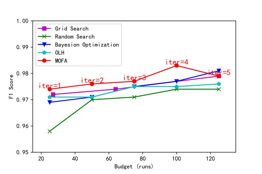
Under review as a conference paper at ICLR 2021

                       p                     p
satisfies D∗ (XLH ) p
                    ≤ 3 d/N and D∗ (XLH ) ≤ 4p d/N is at least 0.965358 and 0.999999 while
D∗ (XRS ) ≤ 16.38 d/N and D∗ (XRS ) ≤ 23.09 d/N with the same probability, respectively.
Robustness. When Ȳ is used as an estimate, the other advantage of Latin Hypercubes is that its
variance will be smaller than the variance of Random Search (Stein, 1987).

Property 3 The variance of Random Search and Latin Hypercubes can be calculated as follows,
            Var(ȲRS ) = N −1 Var[f (X)],      Var(ȲLH ) = N −1 Var[f (X)] − c/n + o(N −1 ),
where c is a non-negative constant. Thus, Latin Hypercubes does asymptotically better than Random
Search.

One advantage of orthogonality is that it makes the estimation of any factor’s main effect unaffected
by their interaction. This can be proved in linear regression by calculating the variance directly.
Besides, orthogonality reduces the order of variance from o(N −1 ) to O(N −3/2 ) (Owen et al., 1994).
Especially for OLH, we have the following result (Owen, 1995).

Property 4 The variance of OLH with strength t = 2 can be calculated as
                       Var(ȲOLH ) = N −1 Var[f (X)] − c/N − c0 /N + O(N −3/2 ),
where c and c0 are non-negative constants. Thus, OLH does asymptotically better than Latin Hyper-
cubes.

In our case, we fix one factor at one level and average other factors to estimate the effect of this factor
at this level. The structure of OLH brings a more accurate estimation of the effect. Consequently, it
is more reliable to make a comparison and make an inference based on the comparison.

4       E MPIRICAL E VALUATION

In this section, we evaluate MOFA in three different settings that involve one two-layer Bayesian
neural network (BNN) and two deep neural networks: Convolutional Neural Networks (CNN) and
Recurrent Neural Networks (RNN). Each model is evaluated on two datasets.

4.1       E XPERIMENT S ETTINGS

Bayesian Neural Networks. We optimize five hyperparameters of a two-layer BNN: the number
of units in layer 1 and layer 2, the step length, the length of the burn-in period, and the momentum
decay. The initial search space for these hyperparameters are set to [24 , 29 ], [24 , 29 ], [10−6 , 10−1 ],
[0, 0.8] and [0, 1] respectively. To ensure the uniformity of hyperparameter search space, we perform
log transformation as the same with Falkner et al. (2018) on the first three hyperparameters. An
open-source code from 2 is used to implement the BNN and the baseline methods. Apart from the
four baselines methods (Random Search, TPE, Hyperband and BOHB) implemented in the code,
we also compare our method with OLH based sampling but without the analyzer for ablation study.
Two different UCI datasets, Boston housing and protein structure described in Hernández-Lobato
& Adams (2015) are used to evaluate the performance. The BNN is trained with Markov Chain
Monte-Carlo (MCMC) sampling and the number of steps for the MCMC sampling is used as the
budgets, we report the negative log-likelihood of the validation data as the final performance.
Deep Neural Networks. We evaluate MOFA for deep neural networks (CNN and RNN) in two prac-
tical tasks: EEG-based intention recognition and IMU-based activity recognition (see Appendix C.1
for details). In this paper, both datasets are divided into a training set (80%) and testing set (20%),
and both tasks are trained with two deep neural network structures: CNN and RNN. The details of
the architecture of the CNN and RNN models are described in Zhang et al. (2019). We optimize
three hyperparameters of these two models: the learning rate lr, the regularization coefficient λ, and
the number of units in each hidden layer. The initial search space we set for the three hyperparameter
is [0.0005, 0.01], [0.0005, 0.01] and [64, 1024] respectively.
    2
        https://github.com/automl/HpBandSter/tree/icml 2018

                                                      6
Under review as a conference paper at ICLR 2021
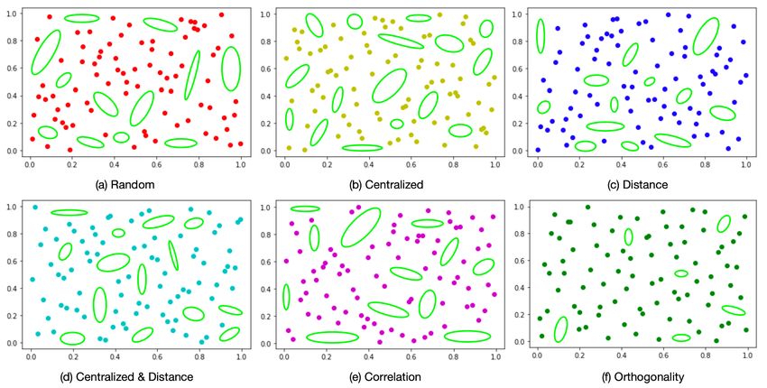
(a) Boston Housing (b) Protein Structure
Figure 2: The negative log-likelihood of BNN on two different UCI datasets.
4.2 H YPERPARAMETER O PTIMIZATION R ESULTS
Overall Results. Fig. 2 shows the HPO results for BNN within two different UCI datasets. We
firstly find that MOFA is significantly better (12%+) than Random Search. For the Boston hous-
ing dataset, the performance of MOFA is even 40% better than that of Random Search when the
budget is limited (Under review as a conference paper at ICLR 2021
(a) CNN (b) RNN
Figure 3: The F1 score of EEG based intention recognition with CNN and RNN.
Method CNN (EEG) CNN (IMU) RNN (EEG) RNN (IMU)
Random 0.851 0.970 0.893 0.957
Centralized 0.841 0.970 0.891 0.953
Distance (Tang, 1998) 0.893 0.972 0.893 0.973
Centralized & Distance 0.882 0.970 0.889 0.969
Correlation (Franco, 2008) 0.913 0.972 0.933 0.977
Orthogonality (Tang, 1993) 0.927 0.976 0.952 0.992
Table 1: The Pick-the-Best performance of different Latin Hypercube sampling methods.
4.4 A NALYSIS AND L IMITATIONS
Model-Free. Apparently, MOFA does not depend on any parametric learning models.
Parallelization. It is easy to calculate the maximum total time that MOFA will take to evaluate in
a parallel way. Assume that the maximum evaluation time for a single configuration is te , where
e is the eth iteration, the number of processes working in parallel is n, the number of iterations is
E, and the number of rows in OLH is N . Then, the maximum total time spent in parallel mode is
PE
T = e=1 te × N/n. Since we assume that all samples spent the maximum time of te , the actual
time spent is much less than T .
Sample Efficiency. Theoretically, the discrepancy of data points can directly affect efficiency.
MOFA uses an OLH-based sampler that preserves better discrepancy than other sampling methods.
Table 1 shows that the HPO performance of OLH outperforms other methods in a single iteration
without factorial analysis. Appendix. C.3 visualize the uniformity of different criteria for Latin
Hypercube construction.
Limitations. MOFA supports both continual and discrete hyperparameters, but it does not apply to
HPO tasks with categorical hyperparameters (e.g. optimizer) since it requires numerical computa-
tion in the transformer. Another issue is that building a proper OLH with hundreds of factors requires
huge computation memory, the space complexity is O(d2 ), where d is the number of factors.
5 C ONCLUSION AND F UTURE W ORK
This paper presents a novel HPO method, MOFA, which enjoys the combined advantages of existing
model-based and model-free HPO methods. It is model-free, parallelizable and sample efficient. To
the best of our knowledge, MOFA is a very first step to exploit factorial design and analysis on HPO,
and more advantaged techniques in these areas can be explored in the future. For example, extending
the method to support tasks with categorical hyperparameters (e.g. optimizer) or tasks with mixed
range size. Another novel direction is to combine model-free sampling with multi-fidelity HPO
methods such as BOHB (Falkner et al., 2018).
8Under review as a conference paper at ICLR 2021
ACKNOWLEDGMENTS
R EFERENCES
Christoph Aistleitner and Markus Hofer. Probabilistic discrepancy bound for monte carlo point sets.
Mathematics of computation, 83(287):1373–1381, 2014.
Christoph Aistleitner, Florian Pausinger, Anne Marie Svane, and Robert F Tichy. On functions of
bounded variation. arXiv preprint arXiv:1510.04522, 2015.
James Bergstra and Yoshua Bengio. Random search for hyper-parameter optimization. The Journal
of Machine Learning Research, 13(1):281–305, 2012.
James S Bergstra, Rémi Bardenet, Yoshua Bengio, and Balázs Kégl. Algorithms for hyper-parameter
optimization. In Advances in neural information processing systems, pp. 2546–2554, 2011.
Dimo Brockhoff, Bernd Bischl, and Tobias Wagner. The impact of initial designs on the perfor-
mance of matsumoto on the noiseless bbob-2015 testbed: A preliminary study. In Proceedings of
the Companion Publication of the 2015 Annual Conference on Genetic and Evolutionary Com-
putation, pp. 1159–1166, 2015.
Ekin D Cubuk, Barret Zoph, Dandelion Mane, Vijay Vasudevan, and Quoc V Le. Autoaugment:
Learning augmentation strategies from data. In Proceedings of the IEEE conference on computer
vision and pattern recognition, pp. 113–123, 2019.
Jacob Devlin, Ming-Wei Chang, Kenton Lee, and Kristina Toutanova. Bert: Pre-training of deep
bidirectional transformers for language understanding. arXiv preprint arXiv:1810.04805, 2018.
Benjamin Doerr, Carola Doerr, and Michael Gnewuch. Probabilistic lower bounds for the discrep-
ancy of latin hypercube samples. In Contemporary Computational Mathematics-A Celebration of
the 80th Birthday of Ian Sloan, pp. 339–350. Springer, 2018.
Michael Drmota and Robert F Tichy. Sequences, discrepancies and applications. Springer, 2006.
Stefan Falkner, Aaron Klein, and Frank Hutter. Bohb: Robust and efficient hyperparameter opti-
mization at scale. arXiv preprint arXiv:1807.01774, 2018.
Matthias Feurer and Frank Hutter. Hyperparameter optimization. In Automated Machine Learning,
pp. 3–33. Springer, Cham, 2019.
Matthias Feurer, Aaron Klein, Katharina Eggensperger, Jost Springenberg, Manuel Blum, and Frank
Hutter. Efficient and robust automated machine learning. In Advances in neural information
processing systems, pp. 2962–2970, 2015.
Jessica Franco. Exploratory designs for computer experiments of complex physical systems simu-
lation. Theses, Ecole Nationale Supérieure des Mines de Saint-Etienne, 2008.
Kaiming He, Georgia Gkioxari, Piotr Dollár, and Ross Girshick. Mask r-cnn. In Proceedings of the
IEEE international conference on computer vision, pp. 2961–2969, 2017.
José Miguel Hernández-Lobato and Ryan Adams. Probabilistic backpropagation for scalable learn-
ing of bayesian neural networks. In International Conference on Machine Learning, pp. 1861–
1869, 2015.
Edmund Hlawka. Discrepancy and riemann integration. Studies in Pure Mathematics, 3, 1971.
Frank Hutter, Holger H Hoos, and Kevin Leyton-Brown. Sequential model-based optimization for
general algorithm configuration. In International conference on learning and intelligent optimiza-
tion, pp. 507–523. Springer, 2011.
Donald R Jones, Matthias Schonlau, and William J Welch. Efficient global optimization of expensive
black-box functions. Journal of Global optimization, 13(4):455–492, 1998.
V Roshan Joseph and Ying Hung. Orthogonal-maximin latin hypercube designs. Statistica Sinica,
pp. 171–186, 2008.
9Under review as a conference paper at ICLR 2021
JF Koksma. Een algemeene stelling uit de theorie der gelijkmatige verdeeling modulo 1. Mathe-
matica B (Zutphen), 11(7-11):43, 1942.
Wolfgang Konen, Patrick Koch, Oliver Flasch, Thomas Bartz-Beielstein, Martina Friese, and Boris
Naujoks. Tuned data mining: a benchmark study on different tuners. In Proceedings of the 13th
annual conference on Genetic and evolutionary computation, pp. 1995–2002, 2011.
Manoj Kumar, George E Dahl, Vijay Vasudevan, and Mohammad Norouzi. Parallel archi-
tecture and hyperparameter search via successive halving and classification. arXiv preprint
arXiv:1805.10255, 2018.
Shindong Lee, BongGu Ko, Keonnyeong Lee, In-Chul Yoo, and Dongsuk Yook. Many-to-many
voice conversion using conditional cycle-consistent adversarial networks. In ICASSP 2020-2020
IEEE International Conference on Acoustics, Speech and Signal Processing (ICASSP), pp. 6279–
6283. IEEE, 2020.
Lisha Li, Kevin Jamieson, Giulia DeSalvo, Afshin Rostamizadeh, and Ameet Talwalkar. Hyperband:
A novel bandit-based approach to hyperparameter optimization. The Journal of Machine Learning
Research, 18(1):6765–6816, 2017.
Chenxi Liu, Barret Zoph, Maxim Neumann, Jonathon Shlens, Wei Hua, Li-Jia Li, Li Fei-Fei, Alan
Yuille, Jonathan Huang, and Kevin Murphy. Progressive neural architecture search. In Proceed-
ings of the European Conference on Computer Vision (ECCV), pp. 19–34, 2018a.
Hanxiao Liu, Karen Simonyan, and Yiming Yang. Darts: Differentiable architecture search. arXiv
preprint arXiv:1806.09055, 2018b.
MD McKay, RJ Beckman, and WJ Conover. Comparison of three methods for selecting values of
input variables in the analysis of output from a computer code. Technometrics, 21(2):239–245,
1979.
Jonas Mockus, Vytautas Tiesis, and Antanas Zilinskas. The application of bayesian methods for
seeking the extremum. Towards global optimization, 2(117-129):2, 1978.
Rahul Mukerjee and CF Jeff Wu. A modern theory of factorial design. Springer Science & Business
Media, 2007.
Art Owen et al. Lattice sampling revisited: Monte carlo variance of means over randomized orthog-
onal arrays. The Annals of Statistics, 22(2):930–945, 1994.
Art B Owen. Randomly permuted (t, m, s)-nets and (t, s)-sequences. In Monte Carlo and quasi-
Monte Carlo methods in scientific computing, pp. 299–317. Springer, 1995.
Joseph Redmon, Santosh Divvala, Ross Girshick, and Ali Farhadi. You only look once: Unified,
real-time object detection. In Proceedings of the IEEE conference on computer vision and pattern
recognition, pp. 779–788, 2016.
Attila Reiss and Didier Stricker. Introducing a new benchmarked dataset for activity monitoring. In
2012 16th International Symposium on Wearable Computers, pp. 108–109. IEEE, 2012.
Michael Stein. Large sample properties of simulations using latin hypercube sampling. Technomet-
rics, 29(2):143–151, 1987.
Christian Szegedy, Vincent Vanhoucke, Sergey Ioffe, Jon Shlens, and Zbigniew Wojna. Rethink-
ing the inception architecture for computer vision. In Proceedings of the IEEE conference on
computer vision and pattern recognition, pp. 2818–2826, 2016.
Boxin Tang. Orthogonal array-based latin hypercubes. Journal of the American statistical associa-
tion, 88(424):1392–1397, 1993.
Boxin Tang. Selecting latin hypercubes using correlation criteria. Statistica Sinica, pp. 965–977,
1998.
10Under review as a conference paper at ICLR 2021
Ashish Vaswani, Noam Shazeer, Niki Parmar, Jakob Uszkoreit, Llion Jones, Aidan N Gomez,
Łukasz Kaiser, and Illia Polosukhin. Attention is all you need. In Advances in neural information
processing systems, pp. 5998–6008, 2017.
CF Jeff Wu and Michael S Hamada. Experiments: planning, analysis, and optimization, volume
552. John Wiley & Sons, 2011.
Quanming Yao, Mengshuo Wang, Yuqiang Chen, Wenyuan Dai, Hu Yi-Qi, Li Yu-Feng, Tu Wei-Wei,
Yang Qiang, and Yu Yang. Taking human out of learning applications: A survey on automated
machine learning. arXiv preprint arXiv:1810.13306, 2018.
Tong Yu and Hong Zhu. Hyper-parameter optimization: A review of algorithms and applications.
arXiv preprint arXiv:2003.05689, 2020.
Xiang Zhang, Xiaocong Chen, Lina Yao, Chang Ge, and Manqing Dong. Deep neural network
hyperparameter optimization with orthogonal array tuning. In International Conference on Neural
Information Processing, pp. 287–295. Springer, 2019.
Yu Zhang, William Chan, and Navdeep Jaitly. Very deep convolutional networks for end-to-end
speech recognition. In 2017 IEEE International Conference on Acoustics, Speech and Signal
Processing (ICASSP), pp. 4845–4849. IEEE, 2017.
Barret Zoph and Quoc V Le. Neural architecture search with reinforcement learning. arXiv preprint
arXiv:1611.01578, 2016.
11Under review as a conference paper at ICLR 2021
A R ELATED W ORK
Model-Based Hyperparameter Optimization. Model-based HPO learns a parametric model such
as a surrogate model or reinforcement learning agent to search optimal hyperparameters guided by
previous experiences. For example, Bayesian Optimization (Mockus et al., 1978) is a sequential
model-based method that tries to find the global optimum with the minimum number of runs, which
balances the exploration and exploitation. Bayesian Optimization is efficient but it highly depends on
the surrogate model that models the objective function. Also, Bayesian Optimization does not allow
for parallelization, since it is a sequential learning-based process. Based on Bayesian Optimization,
optimization with an early-stopping policy such as Successive Halving (SH) (Kumar et al., 2018),
HyperBand (Li et al., 2017), BOHB (Falkner et al., 2018) and ASHA (Bergstra et al., 2011) were
proposed and achieved significant improvements. Different from Bayesian Optimization that uses
Gaussian Process as a surrogate model, TPE (Bergstra et al., 2011) learns a surrogate model with
a graphic structure, which is more suitable in dealing with conditional variables based on its tree-
structure. Reinforcement learning based HPO methods (Zoph & Le, 2016) model with an agent
to learn the policy. It has been used to address NAS (Liu et al., 2018b;a) and data augmentation
problems (Cubuk et al., 2019) in automated machine learning areas. One problem of reinforcement
learning is that it also suffers from exploration and exploitation as well as limits parallelism.
Model-Free Hyperparameter Optimization. Model-free HPO tries to tune hyperparameters with-
out any external learning model. Grid Search is a popularly used model-free HPO method, which
conducts an exhaustive search on all candidate hyperparameter combinations designed by the human
knowledge, it is the most straightforward method to find the optimal combination of hyperparame-
ters. However, the consumption of computational resources of Grid Search increases exponentially
with the increase of the number of hyperparameters and the range of search space. Random Search
(Bergstra et al., 2011) is an improved method of Grid Search, which randomly samples hyperpa-
rameter configurations and can assign a different budget to different samples. Although Random
Search is effective in many machine learning applications, the randomly selected hyperparameters
cannot guarantee to find the global optimum. One advantage of these methods is that hyperparam-
eter configurations can be evaluated in parallel since they run independently of each other (Yu &
Zhu, 2020). More recent literature enhanced random search by using techniques from Experimen-
tal Designs such as space-filling designs (Brockhoff et al., 2015; Konen et al., 2011; Jones et al.,
1998) and OA (Zhang et al., 2019). However, they just used these designs directly without matched
analysis inference. Different from these works, we aim at enhancing hyperparameter optimization
with an orthogonal space-filling technique: OLH (Tang, 1993) and conducting a matched factorial
analysis on it.
B A LGORITHMS
B.1 MOFA: M ODULAR FACTORIAL D ESIGN
In Algorithm 1, we provide the pseudocode for MOFA.
B.2 FACTORIAL A NALYSIS
In Algorithm 2, we provide the pseudocode for factorial analysis.
B.3 OLH C ONSTRUCTION
For a specific HPO task, an OLH with a proper number of factors and levels should be built in
advance. There are many standard construction methods, we use the method proposed by Tang
(1993) to construct OLH, which is described in Algorithm 3. An open-source implementation in R
is provided4 . One basic problem is how to set the proper size for OLH. Here we assume that the
number of rows is at least the square of the number of the range size. For example, in Fig. 1a, there
are three factors and the range size for each hyperparameter is 3, so we construct an OLH with at
least nine rows and three factors. However, it is worth noting that not all the OLH with the square of
the number of range size exists. In that case, we build an OLH with a number of rows that is closest
4
https://github.com/bertcarnell/lhs
12Under review as a conference paper at ICLR 2021
Algorithm 1 Pseudocode of MOFA.
Input: The maximum iteration, E; The importance threshold, β; The range size for each factor, R;
The number of rows (runs) N and columns (factors) F of OLH; The termination condition, C;
The policy for final hyperparameter selection, P ;
Output: The best hyperparameter configuration, θ∗ ; The final performance for the HPO task, π;
1: Initial search space design, S0 ;
2: for each i ∈ [1, E] do
3: Normalizing the initial search space S0 ;
4: Constructing an OLH with Algorithm 3;
5: Hyperparameter sampling with the constructed OLH;
6: Evaluating the sampled configurations in parallel;
7: Building an OLH performance table;
8: Transforming the OLH performance table into an OA;
9: Conducting factorial analysis Algorithm 2 on OA;
10: Reshaping the search space (ROI) into a new space Si ;
11: Updating θ∗ and π;
12: if C is met then
13: Selecting final hyperparameter with P ;
14: Break;
15: end if
16: end forreturn θ∗ , π;
Algorithm 2 Pseudocode for Factorial Analysis.
Input: The input OA, OA(n, p); The threshold, β
Output: New ROI, ROI;
1: Conducting Factorial Performance Analysis;
2: For each factor, pick the range with best mean performance as the best range;
3: Constructing a Factorial Performance Analysis table;
4: Conducting Factorial Importance Analysis based on the selected best range;
5: Constructing a Factorial Importance Analysis table;
6: for each factor f do
7: if importancef < β then
8: Freeze the f with best mean level;
9: end if
10: end forreturn ROI;
Algorithm 3 The construction of OLH.
Input: Let B = (bij ) be a Latin Hypercube of n runs for p factors, with each column being a
permutation of −(n−1)/2, −(n−3)/2, ... , (n−3)/2, (n−1)/2; Let A be an OA(n2 , 2f, n, 2).
Output: The constructed OLH, OLH2 (N, F );
1: For each j, obtain Aj from A by replacing 1, 2, ... , n by b1j , b2j , ... ,bnj respectively, and then
partition Aj as Aj = [Aj1 , ..., Ajf ], where each of Ajk has
two columns;
1 −n
2: For each j, obtain Mj = [Aj1 V, ..., Ajf V ], where V = ;
n 1
3: Obtaining M = [M1 , ..., Mp ], of order N × q, where N = n2 and q = 2pf ;
4: return OLH2 (N, q);
to the square of range size. We also discuss how to set the range size and the number of rows of
OLH in Sec. 3.6.
13Under review as a conference paper at ICLR 2021
(a) CNN (b) RNN
Figure 4: The F1 score of IMU based activity recognition with CNN and RNN.
C S UPPLEMENTARY E XPERIMENTS
C.1 D ETAILS OF DATASET
We use two datasets to evaluate the HPO performance for deep neural networks.
EEG-based Intention Recognition: we use the EEG dataset from PhysioNet eegmmidb database5 ,
where there are 5 different categories. Like in (Zhang et al., 2019), a subset of the dataset (28000
samples) is used in the experiment. The dimension of each sample is 64, which corresponds to 64
channels.
IMU-based Activity Recognition. We use the PAMAP2 dataset6 to conduct the activity recognition
tasks. This dataset is recorded from 18 activities performed by 9 subjects, wearing 3 IMUs and an
HR-monitor. A detailed description of this dataset can be found in (Reiss & Stricker, 2012). To
simplify the training process, we select 8 ADLs as a subset, which is the same with OATM (Zhang
et al., 2019).
C.2 E XPERIMENTAL R ESULTS ON IMU BASED ACTIVITY R ECOGNITION
Fig. 4 shows the HPO results for IMU-based activity recognition. In most cases, MOFA consis-
tently achieves better performance than Random Search, Grid Search and Bayesian Optimization,
although the gap between them decreases as the budgets increase. Since the level of Grid Search is
discrete, its performance is not always better than Random Search, this is one advantage of continual
hyperparameter search than search from a gridded search space. As it shows, overfitting occurred on
CNN when the iteration goes to five. On average, MOFA outperforms Random Search, Grid Search
and Bayesian Optimization with 10%, 8% and 5% improvements respectively.
C.3 U NIFORMITY E VALUATION FOR L ATIN H YPERCUBES
We use the following six criteria of Latin Hypercubes construction for comparison. (1) Random:
Randomly sampling the points within the interval.
(2) Centralized: Sampling points at the center of each interval.
(3) Distance: Maximizing the minimum distance between points.
(4) Centralized & Distance: Maximizing the minimum distance between points, but placing points
at the center of each interval.
(5) Correlation: Minimizing the correlation coefficient between columns.
(6) Orthogonality: OLH based sampling, which is used in our paper.
5
https://www.physionet.org/pn4/EEGmmidb/
6
http://www.pamap.org/demo.html
14Under review as a conference paper at ICLR 2021
Figure 5: The two-dimensional visualization of the samples distribution of Latin Hypercubes sam-
pled with different criteria. For each criterion, the the same number of points were sampled; all of
the dimensions are scaled to range between zero to one. The unfilled areas are marked with green
circles.
For each criterion, we sample the same number of points in a two-dimensional space, all of the
sampled points are scaled to range from zero to one. Fig. 5 shows a visualization of the sample
distribution of Latin Hypercube with different criteria. To show the difference or space-filling prop-
erty more clearly, the unfilled areas are marked with green circles. As it shows, orthogonality has
the best space-filling feature since these circles are smaller than those created by sampling methods
based on other criteria, which means that the sample distribution is more uniform for orthogonality
than for other criteria. We even found that the methods based on the (c) distance and (e) correlation
performed seemed not to perform better than random sampling.
15You can also read