Technical note: Assessment of observation quality for data assimilation in flood models - HESS
←
→
Page content transcription
If your browser does not render page correctly, please read the page content below
Hydrol. Earth Syst. Sci., 22, 3983–3992, 2018
https://doi.org/10.5194/hess-22-3983-2018
© Author(s) 2018. This work is distributed under
the Creative Commons Attribution 4.0 License.

Technical note: Assessment of observation quality
for data assimilation in flood models
Joanne A. Waller1 , Javier García-Pintado1,2 , David C. Mason3 , Sarah L. Dance1 , and Nancy K. Nichols1
1 School of Mathematical, Physical and Computational Sciences, University of Reading, Reading, UK
2 MARUM     – Center for Marine Environmental Sciences and Department of Geosciences, University of Bremen,
Bremen, Germany
3 School of Archaeology, Geography and Environmental Science, University of Reading, Reading, UK

Correspondence: Joanne A. Waller (j.a.waller@reading.ac.uk)

Received: 30 January 2018 – Discussion started: 1 February 2018
Revised: 17 May 2018 – Accepted: 22 May 2018 – Published: 23 July 2018

Abstract. The assimilation of satellite-based water level ob-      1   Introduction
servations (WLOs) into 2-D hydrodynamic models can keep
flood forecasts on track or be used for reanalysis to obtain
improved assessments of previous flood footprints. In either       In data assimilation (DA), observations are combined with
case, satellites provide spatially dense observation fields, but   numerical model output, known as the background, to pro-
with spatially correlated errors. To date, assimilation meth-      vide an accurate description of the current state, known as
ods in flood forecasting either incorrectly neglect the spa-       the analysis. In DA the contributions from the background
tial correlation in the observation errors or, in the best of      and observations are weighted according to their relative un-
cases, deal with it by thinning methods. These thinning meth-      certainty. The observation error statistics are the sum of the
ods result in a sparse set of observations whose error cor-        instrument error and representation error (Janjić et al., 2017).
relations are assumed to be negligible. Here, with a case          The error of representation arises due to the mismatch in the
study, we show that the assimilation diagnostics that make         observation and its model equivalent, and it is often corre-
use of statistical averages of observation-minus-background        lated and state dependent (Waller et al., 2014; Hodyss and
and observation-minus-analysis residuals are useful to es-         Nichols, 2015). In DA, observation error statistics are typ-
timate error correlations in WLOs. The average estimated           ically assumed to be uncorrelated. The data density is re-
correlation length scale of 7 km is longer than the expected       duced in order to satisfy this assumption (Lorenc, 1981). Yet
value of 250 m. Furthermore, the correlations do not decrease      having adequate estimates of these uncertainties is crucial in
monotonically; this unexpected behaviour is shown to be the        order to obtain an accurate analysis. Since the true state of
result of assimilating some anomalous observations. Accu-          the system is not known, the exact observation errors and
rate estimates of the observation error statistics can be used     their statistics can not be calculated. Instead observation un-
to support quality control protocols and provide insight into      certainties must be estimated statistically (e.g. Hollingsworth
which observations it is most beneficial to assimilate. There-     and Lönnberg, 1986; Ueno and Nakamura, 2016). Desroziers
fore, the understanding gained in this paper will contribute       et al. (2005) provide a diagnostic to estimate observation un-
towards the correct assimilation of denser datasets.               certainties using the statistical average of observation-minus-
                                                                   background and observation-minus-analysis residuals. The
                                                                   diagnostic has been applied to operational numerical weather
                                                                   prediction (NWP) settings to estimate observation uncertain-
                                                                   ties (Stewart et al., 2014; Waller et al., 2016a, c; Cordoba
                                                                   et al., 2017). The use of these estimated statistics in NWP re-
                                                                   sults in a more accurate analysis and improvements in objec-

Published by Copernicus Publications on behalf of the European Geosciences Union.
3984 J. A. Waller et al.: Analysis of observation uncertainty for flood assimilation and forecasting
tively measured forecast skill (Weston et al., 2014; Bormann tion of the flood event. It will be seen later that these glob-
et al., 2016; Campbell et al., 2017). ally estimated error statistics show an anomalous pattern. To
The development of DA systems has largely been driven determine the cause of these anomalous results we consider
by its use in NWP, but the methodologies are applicable if observations in different sub-domains have different error
to any system that can be modelled and observed. There characteristics. We also consider if the error statistics differ
have been recent advances in real-time 2-D hydrodynamic for different phases of the flood event. From the results we
modelling and the acquisition and processing of relevant re- infer that the anomalous pattern is not related to the distri-
mote sensing observations (earth observations, EOs) (Raclot, bution of observations over the domain but to observations
2006; Andreadis et al., 2007; Schumann et al., 2007, 2011; during the later stages of the flood. To the best of our knowl-
Mason et al., 2010a, 2012a, 2014). Consequently, several edge this is the first time that the diagnostics have been ap-
studies have shown the benefit of applying DA to operational plied to estimate error statistics for hydrological data assimi-
flood forecasting (Durand et al., 2008, 2014; Montanari et al., lation. Importantly, we show that the diagnostic of Desroziers
2009; Roux and Dartus, 2008; Neal et al., 2009; Matgen et al. (2005) can be used to identify anomalous observation
et al., 2010; Mason et al., 2010b; Giustarini et al., 2011; datasets that are not suitable for assimilation.
García-Pintado et al., 2013, 2015). Grimaldi et al. (2016) re-
view the potential of EOs for inundation mapping and water
level estimation and their use for calibration, validation and 2 The diagnostic of Desroziers et al. (2005)
constraint of real-time hydraulic flood forecasting models.
Data assimilation is a technique used to provide the best es-
A predominant EO technique to obtain water level ob-
timate, the analysis, of the current state of a dynamical sys-
servations (WLOs) is synthetic-aperture radar (SAR). SAR m
tem. The analysis is denoted x a ∈ RN . The analysis is de-
provides high-resolution observations of radar backscatter m
termined by combining the background x b ∈ RN , a model
which, after processing, serve to delineate the flood ex- p
prediction, with observations, y ∈ RN , weighted by their re-
tent. Then, the intersection of the flood extent with a high-
spective error statistics. Here the dimensions of the obser-
resolution lidar digital terrain model is used to obtain the
vation and model state vectors are denoted by N p and N m ,
WLOs. The resulting WLOs are discontinuous but locally
respectively. To compare observations and background it is
dense in space; consequently, the errors in the observations
necessary to project the background into observation space
may be highly correlated. However, the current practice when m p
using the observation operator, H : RN → RN , which may
assimilating WLOs is to neglect the error correlations. To
be non-linear. The analysis can be used to initialize a forecast
make the assumption of uncorrelated errors valid the cur-
which in turn provides a background for the next assimila-
rent approach is to thin the data. Hence, in hydrology, one
tion.
scenario that would benefit from improved understanding
In Desroziers et al. (2005) the analysis is calculated using
of the observation uncertainties is the assimilation of the
−1
satellite-derived water level observations (WLOs) for either
x a = x b + BHT HBHT + R y − H xb ,
operational flood forecast or hindcast analyses (Mason et al.,
2010a; García-Pintado et al., 2013). A more detailed under- = x b + Kd ob , (1)
standing of the observation uncertainties would be highly
where R ∈ R N p ×N p
and B ∈ R N m ×N m
are the observation
useful as understanding the error statistics may permit more
observations to be included in the assimilation, which should and background error covariance matrices, K is the Kalman
allow the information from dense observation sets to be gain matrix and H is defined as the observation operator lin-
fully exploited. Additionally, accurate estimates of observa- earized about the background state. The observation-minus-
tion uncertainties can inform the thinning strategy and sug- background residuals d ob = y − H(x b ), also known as the
gest which observations may benefit the assimilation most innovations, are assumed to be unbiased. Hence any bias
(Fowler et al., 2018). There is a clear potential to improve should be removed before assimilation (Dee, 2005).
the flood forecast if all the SAR WLOs could be assimilated The observation error covariance matrix can be estimated
in an appropriate way. using the observation-minus-background, d ob = y − H(x b ),
In this article we use the diagnostic of Desroziers et al. and observation-minus-analysis, d oa = y − H(x a ), residuals
(2005), described in Sect. 2, to estimate the observation er- (Desroziers et al., 2005). Assuming that the observation and
ror statistics for SAR WLOs that are assimilated using a background errors are mutually uncorrelated, the statistical
local ensemble transform Kalman filter (LETKF) into the expectation of the product of the analysis and background
LISFLOOD-FP 2-D hydrodynamic model. For this study, we residuals is
h T
i
use a sequence of real SAR overpasses in a flood event that E d oa d ob ≈ R. (2)
occurred in November 2012 in SW England. A description of
the SAR WLOs and experimental design are given in Sect. 3. As the resulting matrix is estimated statistically it will not be
Results are discussed in Sect. 4. First, we estimate average symmetric. Therefore, it must be symmetrized before it can
WLO error statistics across the entire domain for the dura- be used in a data assimilation scheme.
Hydrol. Earth Syst. Sci., 22, 3983–3992, 2018 www.hydrol-earth-syst-sci.net/22/3983/2018/J. A. Waller et al.: Analysis of observation uncertainty for flood assimilation and forecasting 3985
The form of the diagnostic in Eq. (2) is not suitable to 3 Methodology
calculate observation error statistics when each assimila-
tion cycle uses different observations. Instead components In this article we estimate the observation error statistics for
of the background and analysis residuals must be paired and SAR WLOs that are assimilated using a LETKF into the
binned, with the binning dependent on the type of correla- LISFLOOD-FP 2-D hydrodynamic model. This study makes
tion being estimated. For example, when calculating spatial use of the observation, model and assimilation system de-
correlations the bins may depend on the distance between ob- scribed in García-Pintado et al. (2015). We direct the reader
servations, whereas for temporal correlations the bins would to this reference, and references therein (particularly Mason
depend on the time between observations. For each bin, β, et al., 2012a, b), for a thorough description of the derivation
the covariance, cov(β), is then computed individually using of WLOs and the assimilation design. Here we summarize
the methodology and provide a description of the data used
Nβ Nβ specifically in this study.
1 X oa ob
1 X
d oa
cov(β) = β di dj − β i k
N k=1 k N k=1
3.1 Derivation of WLOs
Nβ
1 X ob
d , (3) The original observations used in the deviation of WLOs are
N β k=1 j k
obtained using SAR which observes the surface backscatter.
In a SAR image flood water appears dark so long as the sur-
where (d oa ob o
i d j )k is the kth pair of elements of d a and d b
o
face water turbulence is insignificant. Therefore, to obtain
in bin β, and N β is the number of residual pairs in bin β. flood extent, the pixels in a SAR image are grouped into ho-
It is assumed that the observation-minus-background and mogeneous regions. A mean backscatter value is calculated
observation-minus-analysis residuals are unbiased, but this for each region and if this value is below a given threshold,
is not guaranteed. Hence the second term of Eq. (3) ensures the region is classified as flooded. The threshold is deter-
that the computation of the observation error statistics is not mined by using training data from “flood” and “non-flood”
affected by bias (Waller et al., 2016a). To calculate the spa- regions. This initial estimate of flood extent is then refined
tial correlation, the covariance in each bin, cov(β), is divided by, for example, (1) correcting for any high backscatter that
by the estimated variance (the covariance at zero distance, is a result of vegetation either within the flooded region or
cov(0)). at the flood edge; (2) correcting for high backscatter near
The diagnostic in Eqs. (2) and (3) only gives a correct esti- flooded areas that is a result of water with a rough surface;
mate of the observation error uncertainties if the error statis- (3) performing a “nearest neighbour” check, where any local
tics used in the assimilation are exact. Even if the assumed flood height that is significantly larger than those nearby is
statistics are not exact the diagnostic can still provide useful reclassified as non-flooded.
information about the true observation error statistics (Waller To provide the WLOs the refined flood extent is intersected
et al., 2016b; Ménard, 2016). Further limitations include the with high-resolution digital elevation model (DEM). In order
use of an ergodic assumption in order to obtain sufficient to improve the accuracy of the WLOs, they are only calcu-
samples (Todling, 2015) and the assumption that the obser- lated if the slope in the DEM is sufficiently shallow. A fur-
vation operator is linear (Terasaki and Miyoshi, 2014). ther refinement takes into account, for example, the emergent
One further issue is that the standard diagnostic is derived vegetation at the flood edge.
assuming that the analysis is calculated using minimum vari- The WLO derivation process results in a large number of
ance linear statistical estimation. If local ensemble DA is WLOs that exist in clusters. It is expected that many of the
used to determine the analysis, the diagnostic does not result observations in a cluster will be highly correlated and hence
in a correct estimate of the observation uncertainties. How- not contribute independent information. At this stage in the
ever, by using a modified version of the diagnostic some of processing, Mason et al. (2012a) thin the WLOs to reduce
the observation error statistics may be estimated. It is possi- spatial correlation. However, we postpone this step until after
ble to estimate the error correlations between two observa- the quality control procedures for the data assimilation have
tions if the observation operator that determines the model been performed.
equivalent of observation y i acts only on states that have
been updated using the observation y j (Waller et al., 2017). 3.2 Model and data assimilation
Since we use a LETKF assimilation scheme in this study, we
must take this into account when estimating observation er- The observations are assimilated into a 75 m resolution
ror statistics for the WLOs. LISFLOOD-FP flood simulation model (Bates and Roo,
2000) using a LETKF (Hunt et al., 2007). Due to the formula-
tion with the diagnostic described in Sect. 2, the localization
in the LETKF is set in standard 2-D Euclidean space rather
than the physically based distance along the river channel
www.hydrol-earth-syst-sci.net/22/3983/2018/ Hydrol. Earth Syst. Sci., 22, 3983–3992, 20183986 J. A. Waller et al.: Analysis of observation uncertainty for flood assimilation and forecasting
described in García-Pintado et al. (2015), which would re- 3.4 Potential observation error sources
quire a further adaptation of the diagnostic calculation. The
localization radius is set using a compactly supported fifth- In data assimilation the observation uncertainty has contri-
order piecewise rational function (Gaspari and Cohn, 1999, butions from both measurement errors and representation er-
Eq. 4.10) with length scale 20 km. rors. The representation error arises due to the difference be-
To compare the modelled field with the observed quantity tween an actual observation and the modelled representation
it is necessary to define an observation operator that maps of an observation; this difference can be a result of the fol-
from model to observation space. In this study we use the lowing:
“nearest wet pixel” approach described in García-Pintado
– Pre-processing/QC errors are errors introduced during
et al. (2013). The mapping in the nearest wet pixel approach
the observation pre-processing or quality control proce-
is dependent on the inundation status at the model location.
dures.
If at an observation location the model is flooded, the model
equivalent of the observation is simply the water level pre- – Observation operator errors are errors that arise due to
dicted by the model. However, if the model is dry at the ob- approximations in the mapping between model and ob-
servation location the model equivalent of the observation is servation space.
taken to be the model water level at the wet pixel nearest to
the observation location. – Errors due to unresolved scales and processes are er-
rors that result from the mismatch between the scales
3.3 Quality control and data thinning represented in the model field and the observations.
Data assimilation techniques can lose accuracy if presented For the WLOs it is clear that a pre-processing error will
with an observation that is grossly inconsistent with the exist as there is potential for errors to be introduced in the
model state (Vanden-Eijnden and Weare, 2013). Thus, before derivation of the WLOs. For example if the water surface is
being assimilated, the WLOs are subjected to several quality rough it may be assumed that the pixel is dry; as a result the
control (QC) protocols according to the physical characteris- flood extent would be incorrect and hence an error would be
tics of the terrain and land cover. An additional background introduced in the WLO. For nearby pixels it is possible that
check is performed where observations that result in anoma- there will be similar errors in the derivation process, thereby
lous observation-minus-background residuals are discarded. introducing correlated observation errors. The procedures in
The QC procedures result in dense cluster of discontinuous Mason et al. (2012a) provide an estimated standard deviation
observations in which both the observations and their errors for the WLO pre-processing error and thin the data to ensure
may be highly correlated. A direct assimilation of this dense that the pre-processing error is uncorrelated. However, we
dataset would lead to an analysis biased towards the obser- note that in this study we use a denser dataset than is typically
vations and, for covariance-evolving methods (e.g. ensemble produced. Therefore, there is potential for some correlated
Kalman filters), an over-reduced posterior covariance and un- pre-processing error to remain.
stable long-term forecast/assimilation cycles. Thus, to reduce A potential source of correlated error for WLOs is the ob-
the number of correlated observations and to avoid dealing servation operator error. As described in Sect. 3.2 the obser-
with the spatial correlation in the assimilation, the current vation operator uses the “nearest wet pixel” approach. For
approach is to further thin the data (as is standard in other observations in locations where the model is flooded it is ex-
assimilation applications such as NWP and oceanography; pected that there is minimal error in the observation operator
Dando et al., 2007; Li et al., 2010). The applied thinning, as (since the corresponding water level is predicated directly by
described in Mason et al. (2012a), uses a top down cluster- the model). However, if the observation location does not co-
ing approach in which principal component analysis is used incide with a flooded model pixel it is necessary to find the
to select observations that have the highest information con- nearest wet pixel in the model. It is possible that in locating
tent. The spatial autocorrelation of the resulting observations the nearest wet pixel and extrapolating information we intro-
is calculated, and if any significant correlation exists the thin- duce correlated error.
ning procedure is applied iteratively until no significant cor- The error due to unresolved scales and processes is also
relation remains. Typically the thinned dataset contains ap- a possible source of observation error correlations. Although
proximately 1 % of the pre-thinned observations. The mea- in this case the model is of relatively high resolution com-
sured standard deviation for the thinned dataset can be cal- pared to the observation resolution, there are still scales that
culated by fitting a plane by linear regression to the WLOs. are unresolved. Previous studies that have considered these
The variance of the difference between the WLO and planar scale mismatch errors have found that they are typically cor-
surface can be used as an estimate of the observation error related (Janjić and Cohn, 2006; Waller et al., 2014; Hodyss
variance. This approach is considered adequate for this case and Nichols, 2015).
study as the floodplain in the downstream observed areas is
reasonably flat.
Hydrol. Earth Syst. Sci., 22, 3983–3992, 2018 www.hydrol-earth-syst-sci.net/22/3983/2018/J. A. Waller et al.: Analysis of observation uncertainty for flood assimilation and forecasting 3987
3.5 Calculation of WLO error statistics – an underestimated standard deviation
We estimate observation uncertainties for observations from – an underestimated correlation length scale.
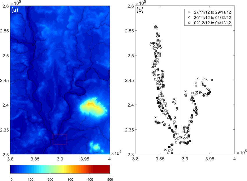
a real flood event that occurred in West England on an area Therefore, we would expect the true standard deviations and
of the lower Severn and Avon rivers in November 2012 length scales to be larger than those we estimate using the
(Fig. 1a). The WLOs were extracted from a sequence of diagnostic.
seven satellite SAR observations (acquired by the COSMO-
SkyMed constellation) using the method described in Mason
et al. (2012a). During the flood event the WLOs are available 4 Results
daily for the period 27 November to 4 December 2012 (with
the exception of 3 December). Observations on the first day 4.1 Average observation error statistics
illustrate the flood levels just before the flood peak in the Sev-
We first estimate average horizontal error covariances across
ern. On 30 November the river went back in bank; however, a
the entire domain for the duration of the flood event. We plot
substantial amount of water remained on the floodplain (see
in Fig. 2 the estimated correlation, along with the number of
Fig. 2 in García-Pintado et al., 2015).
samples used, for the WLOs.
Before being assimilated, the WLOs are subject to the QC
The estimated statistics give a standard deviation of 54 cm.
and thinning procedures described in Sect. 3.3. When used
This is slightly lower that the assumed error standard devia-
in previous studies such as García-Pintado et al. (2015) the
tion of 59 cm. Following the theory of Waller et al. (2016b)
dataset has been thinned to a separation distance of 250 m,
we expect the estimated standard deviation to be an under-
at which the observation errors are assumed uncorrelated.
estimate of the true observation error standard deviation, and
However, in this article a denser observation set (although
hence the results suggest that the assumed standard deviation
still sparse) with thinning distance of 125 m is used, in which
is likely set at the correct level.
some spatial correlation should remain. The location of the
Our results show that the correlations become insignificant
observations is plotted in Fig. 1b.
(< 0.2) at approximately 8 km, but there is some unexpected
We apply the diagnostic of Desroziers et al. (2005) to
behaviour before 8 km. The correlations drop smoothly be-
the observation-minus-background and observation-minus-
tween 0 and 4 km then increase again up to 6 km before
analysis residuals resulting from the flood assimilation. We
dropping off. This behaviour is seen for a variety of different
first use all available data to calculate the average horizon-
binning widths (not shown). We investigate the cause of this
tal error variance and correlations. We then consider if the
“local maximum” in the estimated correlations in Sects. 4.2
observations of the flood on the Severn are similar to the er-
and 4.3. In general we find that the correlation distance is
ror statistics for the Avon. Finally we consider if the error
much longer than the thinning distance of 125 m, which was
statistics vary for different periods of the flood. For all cases
chosen to try to ensure that the observation errors are un-
the observation error correlations are calculated at a 1 km bin
correlated. Furthermore, theoretical results of Waller et al.
spacing. As we use an LETKF we must use a modified form
(2016b) suggest that, with this design of assimilation experi-
of the diagnostic (see Sect. 2). As a result we are not able to
ment, the correlation length scales will be underestimated.
calculate observation error correlations for observation pairs
with a separation distance greater than 19 km. When evaluat- 4.2 Correlations in different parts of the domain
ing the correlations we assume that they become insignificant
when they drop below 0.2 (Liu and Rabier, 2002). It is possible that the local maximum in the correlations is a
For this assimilation system we assume that the ensemble result of observations on different tributaries of the river. To
background error covariance matrix gives a reasonable es- test this hypothesis we split the domain in two (as shown in
timate of the true background error statistics. The assumed Fig. 1): the western domain covering the river Severn and
standard deviation for the WLOs is 59 cm; this is calculated eastern domain covering the river Avon. We plot the esti-
as described in Sect. 3.3. The value accounts only for the pre- mated correlations, along with the number of samples used
processing error, and not for any error introduced by the ap- for the SAR WLOs, for the western part of the domain in
proximations in the observation operator or scale mismatch Fig. 3 and for the eastern part of the domain in Fig. 4. We
errors and, therefore, may be an underestimate of the true note that there are fewer observations in the eastern domain.
error standard deviation. This results in fewer available samples for the calculation in
As is typical for most DA systems, the observation errors Eq. (3) and hence the results are subject to greater sampling
are assumed uncorrelated. With these assumed error statistics error.
the theoretical work of Waller et al. (2016b) suggests that From Figs. 3 and 4 we see that the “local maximum” in
the observation error statistics estimated using the diagnostic the correlations is still present in both parts of the domain. In
will have the following: the eastern domain it is very pronounced. This suggests that
the cause of the increase in correlations between 4 and 6 km
is not observations on different tributaries of the river.
www.hydrol-earth-syst-sci.net/22/3983/2018/ Hydrol. Earth Syst. Sci., 22, 3983–3992, 20183988 J. A. Waller et al.: Analysis of observation uncertainty for flood assimilation and forecasting
Figure 1. (a) Flood model domain where the colour bar denotes the height in metres and (b) position of SAR WLOs on OSGB 1936
British National Grid projection; coordinates in metres. For (b) the line denotes the west/east domain split discussed in Sect. 4.2, crosses:
27–29 November, circles: 30 November and 1 December, squares: 2 and 4 December.
1 5000 1 2500
Number of obs pairs
Number of obs pairs
0.8 4000 0.8 2000
Correlation
Correlation
0.6 3000 0.6 1500
0.4 2000 0.4 1000
0.2 1000 0.2 500
0 0 0 0
0 2 4 6 8 10 12 14 16 18 20 0 2 4 6 8 10 12 14 16 18 20
Separation distance (km) Separation distance (km)
Figure 2. Estimated SAR WLO error correlations (black line) and Figure 3. Estimated SAR WLO error correlations (black line) and
number of samples (bars) used for the calculation. Estimated error number of samples (bars) used (bin width = 1 km), west domain.
standard deviation is 54 cm. Estimated error standard deviation is 58 cm.
4.3 Correlations at different times bank; for this period the standard deviation is largest, as is the
correlation length scale, which is approximately 8 km. It is
We next consider if the correlation structure changes over also in this final period where the “local maximum” appears
time. We plot in Figs. 5, 6 and 7 the correlations calculated in the correlations.
for the first three days, the second two days and the final Figure 7 shows the estimated error statistics for the reces-
two days respectively. At the beginning of the flood period, sion stages for the flood. During this period a high proportion
the observations have similar standard deviations to those es- of the observations were in areas which remained flooded but
timated for the entire flood event; however, the correlation were disconnected from the main river flow. For this same
length scale is short, approximately 2 km. sequence of SAR overpasses García-Pintado et al. (2015)
During the middle of the flood event the observation error showed that the assimilation of the last three overpasses was
standard deviation decreases and the correlation length scale still able to exploit the background ensemble covariances to
increases slightly. For the final two days the river is back in pass some of the information from these WLOs to the main
Hydrol. Earth Syst. Sci., 22, 3983–3992, 2018 www.hydrol-earth-syst-sci.net/22/3983/2018/J. A. Waller et al.: Analysis of observation uncertainty for flood assimilation and forecasting 3989
1 2500 1 2500
Number of obs pairs
Number of obs pairs
0.8 2000 0.8 2000
Correlation
Correlation
0.6 1500 0.6 1500
0.4 1000 0.4 1000
0.2 500 0.2 500
0 0 0 0
0 2 4 6 8 10 12 14 16 18 20 0 2 4 6 8 10 12 14 16 18 20
Separation distance (km) Separation distance (km)
Figure 4. Estimated SAR WLO error correlations (black line) and Figure 6. Estimated SAR WLO error correlations (black line) and
number of samples (bars) used (bin width = 1 km), east domain. Es- number of samples (bars) used (bin width = 1 km), 30 November
timated error standard deviation is 43 cm. and 1 December. Estimated error standard deviation is 43 cm.
1 2500 1 2500
Number of obs pairs
Number of obs pairs
0.8 2000 0.8 2000
Correlation
Correlation
0.6 1500 0.6 1500
0.4 1000 0.4 1000
0.2 500 0.2 500
0 0 0 0
0 2 4 6 8 10 12 14 16 18 20 0 2 4 6 8 10 12 14 16 18 20
Separation distance (km) Separation distance (km)
Figure 5. Estimated SAR WLO error correlations (black line) and Figure 7. Estimated SAR WLO error correlations (black line) and
number of samples (bars) used (bin width = 1 km), 27–29 Novem- number of samples (bars) used (bin width = 1 km), 2 and 4 Decem-
ber. Estimated error standard deviation is 53 cm. ber. Estimated error standard deviation is 57 cm.
flow. However, two effects became evident: (a) the assimi- 5 Conclusions
lation increments were of a smaller magnitude in these last
stages, and (b) the corrections to the flow in these last stages We have shown that the Desroziers et al. (2005) diagnostic is
were gradually more short-lived. This was a result of the re- a useful tool to identify the error covariance in WLOs from
duced information content in these WLOs regarding the in- satellite SAR. Further, the diagnostic has been able, in the
flow errors upstream, which in the end control the flood and case study, to isolate an unexpected anomaly in the correla-
flow evolution. Here the Desroziers et al. (2005) diagnostic tion structure, pointing to the applicability limits of the satel-
has been able to identify a corresponding anomalous struc- lite WLOs in the flood plain in the recession stages of the
ture in the WLO errors at these last stages. The correlation flood. The diagnostic has been useful in this study for high-
structure shown in Fig. 7 indicates that apart from the longer lighting anomalous data. Given its low-cost calculation, we
correlation errors, which can be expected from the smoother propose it be customarily calculated in flood forecasts and
flood dynamics at the end of the flood, an increase in the cor- hindcast analyses to support the understanding of the obser-
relation appears at ∼ 6 km. The increasing disconnection of vation errors and to support QC protocols for selection of
the WLOs in the flood plain from the main flow appears to adequate observations. However, due to the dependence of
be the cause for the local maximum in the estimated corre- the observation error on the choice of observation operator
lation structure. However, further work is required to deter- and model resolution, results will differ for each individual
mine why the “local maximum” in the estimated correlation user. Therefore, further study may be required to understand
function appears at 6 km. how the diagnostic results can best support QC protocols.
Data availability. The data used in this study are available in
García-Pintado (2018).
www.hydrol-earth-syst-sci.net/22/3983/2018/ Hydrol. Earth Syst. Sci., 22, 3983–3992, 20183990 J. A. Waller et al.: Analysis of observation uncertainty for flood assimilation and forecasting
Author contributions. JW, JG-P and DM prepared the data and ran Durand, M., Andreadis, K. M., Alsdorf, D. E., Lettenmaier, D.
the experiments. JW and JG-P analysed the results and drafted the P., Moller, D., and Wilson, M.: Estimation of bathymetric
manuscript. DM, SD and NN contributed to the discussion and depth and slope from data assimilation of swath altimetry
manuscript editing. into a hydrodynamic model, Geophys. Res. Lett., 35, L20401,
https://doi.org/10.1029/2008GL034150, 2008.
Durand, M., Neal, J., Rodríguez, E., Andreadis, K. M., Smith,
Competing interests. The authors declare that they have no conflict L. C., and Yoon, Y.: Estimating reach-averaged discharge
of interest. for the River Severn from measurements of river wa-
ter surface elevation and slope, J. Hydrol., 511, 92–104,
https://doi.org/10.1016/j.jhydrol.2013.12.050, 2014.
Acknowledgements. Joanne A. Waller, Nancy K. Nichols García-Pintado, J.: DEMON: Simulation output from en-
and Sarah L. Dance were supported in part by UK NERC semble assimilation of Synthetic Aperture Radar (SAR)
grants NE/K008900/1 (FRANC), NE/N006682/1 (OSCA). water level observations into the Lisflood-FP flood fore-
Joanne A. Waller and Sarah L. Dance received additional support cast model, Centre for Environmental Data Analysis,
from UK EPSRC grant EP/P002331/1 (DARE). Nancy K. Nichols https://doi.org/10.5285/b43ce022c8f94f79b5c3b3ede7aad975,
was also supported by the UK NERC National Centre for Earth 2018.
Observation (NCEO). Javier García-Pintado, David C. Mason and Fowler, A., Dance, S., and Waller, J.: On the interaction of observa-
Sarah L. Dance were supported by UK NERC grants NE/1005242/1 tion and prior error correlations in data assimilation, Q. J. Roy.
(DEMON) and NE/K00896X/1 (SINATRA). The data used in this Meteorol. Soc., 144, 48–62, https://doi.org/10.1002/qj.3183,
study may be obtained on request, subject to licensing conditions, 2018.
by contacting the corresponding author. García-Pintado, J., Neal, J. C., Mason, D. C., Dance, S.
L., and Bates, P. D.: Scheduling satellite-based SAR ac-
Edited by: Florian Pappenberger quisition for sequential assimilation of water level obser-
Reviewed by: two anonymous referees vations into flood modelling, J. Hydrol., 495, 252–266,
https://doi.org/10.1016/j.jhydrol.2013.03.050, 2013.
García-Pintado, J., Mason, D., Dance, S., Cloke, H., Neal, J.,
Freer, J., and Bates, P.: Satellite-supported flood forecasting in
References river networks: A real case study, J. Hydrol., 523, 706–724,
https://doi.org/10.1016/j.jhydrol.2015.01.084, 2015.
Andreadis, K. M., Clark, E. A., Lettenmaier, D. P., and Als- Gaspari, G. and Cohn, S. E.: Construction of correlation functions
dorf, D. E.: Prospects for river discharge and depth esti- in two and three dimensions, Q. J. Roy. Meteorol. Soc., 125, 723–
mation through assimilation of swath-altimetry into a raster- 757, 1999.
based hydrodynamics model, Geophys. Res. Lett., 34, L10403, Giustarini, L., Matgen, P., Hostache, R., Montanari, M., Plaza, D.,
https://doi.org/10.1029/2007GL029721, 2007. Pauwels, V. R. N., De Lannoy, G. J. M., De Keyser, R., Pfister, L.,
Bates, P. and Roo, A. D.: A simple raster-based model Hoffmann, L., and Savenije, H. H. G.: Assimilating SAR-derived
for flood inundation simulation, J. Hydrol., 236, 54–77, water level data into a hydraulic model: a case study, Hydrol.
https://doi.org/10.1016/S0022-1694(00)00278-X, 2000. Earth Syst. Sci., 15, 2349–2365, https://doi.org/10.5194/hess-15-
Bormann, N., Bonavita, M., Dragani, R., Eresmaa, R., Ma- 2349-2011, 2011.
tricardi, M., and McNally, A.: Enhancing the impact of Grimaldi, S., Li, Y., Pauwels, V. R. N., and Walker, J. P.: Remote
IASI observations through an updated observation-error co- Sensing-Derived Water Extent and Level to Constrain Hydraulic
variance matrix, Q. J. Roy. Meteorol. Soc., 142, 1767–1780, Flood Forecasting Models: Opportunities and Challenges, Surv.
https://doi.org/10.1002/qj.2774, 2016. Geophys., 37, 977–1034, https://doi.org/10.1007/s10712-016-
Campbell, W. F., Satterfield, E. A., Ruston, B., and Baker, N. 9378-y, 2016.
L.: Accounting for Correlated Observation Error in a Dual- Hodyss, D. and Nichols, N. K.: The error of repre-
Formulation 4D Variational Data Assimilation System, Mon. sentation: basic understanding, Tellus A, 67, 24822,
Weather Rev., 145, 1019–1032, https://doi.org/10.1175/MWR- https://doi.org/10.3402/tellusa.v67.24822, 2015.
D-16-0240.1, 2017. Hollingsworth, A. and Lönnberg, P.: The statistical struc-
Cordoba, M., Dance, S., Kelly, G., Nichols, N., and Waller, J.: Di- ture of short-range forecast errors as determined from ra-
agnosing Atmospheric Motion Vector observation errors for an diosonde data. Part I: The wind field, Tellus A, 38, 111–136,
operational high resolution data assimilation system, Q. J. Roy. https://doi.org/10.1111/j.1600-0870.1986.tb00460.x, 1986.
Meteorol. Soc., 143, 333–341, https://doi.org/10.1002/qj.2925, Hunt, B. R., Kostelich, E. J., and Szunyogh, I.: Efficient
2017. data assimilation for spatiotemporal chaos: A local en-
Dando, M., Thorpe, A., and Eyre, J.: The optimal density of atmo- semble transform Kalman filter, Physica D, 230, 112–126,
spheric sounder observations in the Met Office NWP system, Q. https://doi.org/10.1016/j.physd.2006.11.008, 2007.
J. Roy. Meteorol. Soc., 133, 1933–1943, 2007. Janjić, T. and Cohn, S. E.: Treatment of Observation Error due
Dee, D. P.: Bias and data assimilation, Q. J. Roy. Meteorol. Soc., to Unresolved Scales in Atmospheric Data Assimilation, Mon.
131, 3323–3343, https://doi.org/10.1256/qj.05.137, 2005. Weather Rev., 134, 2900–2915, 2006.
Desroziers, G., Berre, L., Chapnik, B., and Poli, P.: Diagnosis of ob- Janjić, T., Bormann, N., Bocquet, M., Carton, J. A., Cohn, S. E.,
servation, background and analysis-error statistics in observation Dance, S. L., Losa, S. N., Nichols, N. K., Potthast, R., Waller, J.
space, Q. J. Roy. Meteorol. Soc., 131, 3385–3396, 2005.
Hydrol. Earth Syst. Sci., 22, 3983–3992, 2018 www.hydrol-earth-syst-sci.net/22/3983/2018/J. A. Waller et al.: Analysis of observation uncertainty for flood assimilation and forecasting 3991 A., and Weston, P.: On the representation error in data assimila- 27, 2553–2574, https://doi.org/10.1080/01431160600554397, tion, Q. J. Roy. Meteorol. Soc., https://doi.org/10.1002/qj.3130, 2006. in press, 2017. Roux, H. and Dartus, D.: Sensitivity Analysis and Predic- Li, X., Zhu, J., Xiao, Y., and Wang, R.: A Model-Based tive Uncertainty Using Inundation Observations for Param- Observation-Thinning Scheme for the Assimilation of eter Estimation in Open-Channel Inverse Problem, J. Hy- High-Resolution SST in the Shelf and Coastal Seas draul. Eng., 134, 541–549, https://doi.org/10.1061/(ASCE)0733- around China, J. Atmos. Ocean. Tech., 27, 1044–1058, 9429(2008)134:5(541), 2008. https://doi.org/10.1175/2010JTECHO709.1, 2010. Schumann, G. J.-P., Hostache, R., Puech, C., Hoffmann, L., Mat- Liu, Z.-Q. and Rabier, F.: The interaction between model resolution gen, P., Pappenberger, F., and Pfister, L.: High-Resolution 3-D observation resolution and observation density in data assimila- Flood Information From Radar Imagery for Flood Hazard Man- tion: A one dimensional study, Q. J. Roy. Meteorol. Soc., 128, agement, IEEE T. Geosci. Remote, 45, 1715–1725, 2007. 1367–1386, 2002. Schumann, G. J.-P., Neal, J. C., Mason, D. C., and Bates, P. Lorenc, A. C.: A global three-dimensional multivariate statistical D.: The accuracy of sequential aerial photography and SAR interpolation scheme, Mon. Weather Rev., 109, 701–721, 1981. data for observing urban flood dynamics, a case study of the Mason, D. C., Speck, R., Deveraux, B., Schumann, G., Neal, J., UK summer 2007 floods, Remote Sens. Environ., 115, 2536– and Bates, P.: Flood detection in urban areas using TerraSAR-X, 2546, https://doi.org/10.1016/j.rse.2011.04.039, 2011. IEEE T. Geosci. Remote, 48, 882–894, 2010a. Stewart, L. M., Dance, S. L., Nichols, N. K., Eyre, J. Mason, D. C., Schumann, G., and Bates, P. D.: Data Uti- R., and Cameron, J.: Estimating interchannel observation- lization in Flood Inundation Modelling, in: Flood Risk error correlations for IASI radiance data in the Met Of- Science and Management, edited by: Pender, G. and fice system, Q. J. Roy. Meteorol. Soc., 140, 1236–1244, Faulkner, H., Wiley-Blackwell, Chichester, 209–233, https://doi.org/10.1002/qj.2211, 2014. https://doi.org/10.1002/9781444324846.ch11, 2010b. Terasaki, K. and Miyoshi, T.: Data Assimilation with Error- Mason, D. C., Schumann, G. J.-P., Neal, J., Garcia-Pintado, J., and Correlated and Non-Orthogonal Observations: Experi- Bates, P.: Automatic near real-time selection of flood water levels ments with the Lorenz-96 Model, SOLA, 10, 210–213, from high resolution Synthetic Aperture Radar images for assim- https://doi.org/10.2151/sola.2014-044, 2014. ilation into hydraulic models: A case study, Remote Sens. En- Todling, R.: A complementary note to ‘A lag-1 smoother approach viron., 124, 705–716, https://doi.org/10.1016/j.rse.2012.06.017, to system-error estimation’: the intrinsic limitations of resid- 2012a. ual diagnostics, Q. J. Roy. Meteorol. Soc., 141, 2917–2922, Mason, D. C., Davenport, I. J., Neal, J. C., Schumann, G. J. https://doi.org/10.1002/qj.2546, 2015. P., and Bates, P. D.: Near Real-Time Flood Detection in Ur- Ueno, G. and Nakamura, N.: Bayesian estimation of the ban and Rural Areas Using High-Resolution Synthetic Aper- observation-error covariance matrix in ensemble-based ture Radar Images, IEEE T. Geosci. Remote, 50, 3041–3052, filters, Q. J. Roy. Meteorol. Soc., 142, 2055–2080, https://doi.org/10.1109/TGRS.2011.2178030, 2012b. https://doi.org/10.1002/qj.2803, 2016. Mason, D. C., Giustarini, L., Garcia-Pintado, J., and Cloke, Vanden-Eijnden, E. and Weare, J.: Data Assimilation in the H.: Detection of flooded urban areas in high resolu- Low Noise Regime with Application to the Kuroshio, Mon. tion Synthetic Aperture Radar images using double scat- Weather Rev., 141, 1822–1841, https://doi.org/10.1175/MWR- tering, Int. J. Appl. Earth Obs. Geoinf., 28, 150–159, D-12-00060.1, 2013. https://doi.org/10.1016/j.jag.2013.12.002, 2014. Waller, J. A., Dance, S. L., Lawless, A. S., Nichols, N. K., and Eyre, Matgen, P., Montanari, M., Hostache, R., Pfister, L., Hoffmann, L., J. R.: Representativity error for temperature and humidity using Plaza, D., Pauwels, V. R. N., De Lannoy, G. J. M., De Keyser, the Met Office high-resolution model, Q. J. Roy. Meteorol. Soc., R., and Savenije, H. H. G.: Towards the sequential assimilation 140, 1189–1197, https://doi.org/10.1002/qj.2207, 2014. of SAR-derived water stages into hydraulic models using the Par- Waller, J. A., Ballard, S. P., Dance, S. L., Kelly, G., ticle Filter: proof of concept, Hydrol. Earth Syst. Sci., 14, 1773– Nichols, N. K., and Simonin, D.: Diagnosing Horizontal 1785, https://doi.org/10.5194/hess-14-1773-2010, 2010. and Inter-Channel Observation Error Correlations for SE- Ménard, R.: Error covariance estimation methods based on analysis VIRI Observations Using Observation-Minus-Background and residuals: theoretical foundation and convergence properties de- Observation-Minus-Analysis Statistics, Remote Sensing, 8, 581, rived from simplified observation networks, Q. J. Roy. Meteorol. https://doi.org/10.3390/rs8070581, 2016a. Soc., 142, 257–273, https://doi.org/10.1002/qj.2650, 2016. Waller, J. A., Dance, S. L., and Nichols, N. K.: Theoret- Montanari, M., Hostache, R., Matgen, P., Schumann, G., Pfister, ical insight into diagnosing observation error correlations L., and Hoffmann, L.: Calibration and sequential updating of using observation-minus-background and observation-minus- a coupled hydrologic-hydraulic model using remote sensing- analysis statistics, Q. J. Roy. Meteorol. Soc., 142, 418–431, derived water stages, Hydrol. Earth Syst. Sci., 13, 367–380, https://doi.org/10.1002/qj.2661, 2016b. https://doi.org/10.5194/hess-13-367-2009, 2009. Waller, J. A., Simonin, D., Dance, S. L., Nichols, N. K., Neal, J., Schumann, G., Bates, P., Buytaert, W., Matgen, P., and and Ballard, S. P.: Diagnosing observation error correlations Pappenberger, F.: A data assimilation approach to discharge esti- for Doppler radar radial winds in the Met Office UKV mation from space, Hydrol. Process., 23, 3641–3649, 2009. model using observation-minus-background and observation- Raclot, D.: Remote sensing of water levels on floodplains: a spatial minus-analysis statistics, Mon. Weather Rev., 144, 3533–3551, approach guided by hydraulic functioning, Int. J. Remote Sens., https://doi.org/10.1175/MWR-D-15-0340.1, 2016c. www.hydrol-earth-syst-sci.net/22/3983/2018/ Hydrol. Earth Syst. Sci., 22, 3983–3992, 2018
3992                         J. A. Waller et al.: Analysis of observation uncertainty for flood assimilation and forecasting

Waller, J. A., Dance, S. L., and Nichols, N. K.: On diag-          Weston, P. P., Bell, W., and Eyre, J. R.: Accounting for
  nosing observation error statistics in localized ensemble data     correlated error in the assimilation of high-resolution
  assimilation, Q. J. Roy. Meteorol. Soc., 143, 2677–2686,           sounder data, Q. J. Roy. Meteorol. Soc., 140, 2420–2429,
  https://doi.org/10.1002/qj.3117, 2017.                             https://doi.org/10.1002/qj.2306, 2014.

Hydrol. Earth Syst. Sci., 22, 3983–3992, 2018                                  www.hydrol-earth-syst-sci.net/22/3983/2018/
You can also read