Empirical path and station corrections for surface-wave magnitude, Ms, using a global network
←
→
Page content transcription
If your browser does not render page correctly, please read the page content below
Geophys. J. Int. (2003) 155, 379–390

Empirical path and station corrections for surface-wave magnitude,
M s , using a global network

Neil D. Selby, David Bowers, Peter D. Marshall and Alan Douglas
AWE Blacknest, Brimpton, Reading RG7 4RS. E-mail: neil@blacknest.gov.uk

Accepted 2003 April 30. Received 2003 April 28; in original form 2001 November 19

                                       SUMMARY
                                       One of the most commonly used methods of estimating the size of shallow earthquakes is the
                                       surface-wave magnitude scale, M s . It has been known since the inception of the scale that the
                                       M s of a seismic disturbance recorded at different stations can vary due to path propagation and
                                       station terms, but it has been difficult to quantify these variations on a global basis because,
                                       until recently, there has been no attempt to record M s in a uniform way on a worldwide network.

                                                                                                                                                       Downloaded from http://gji.oxfordjournals.org/ by guest on May 9, 2015
                                          Here we use M s measurements within the Reviewed Event Bulletin (REB) of the International
                                       Data Centre (IDC) which is produced to help monitor compliance with the Comprehensive
                                       Nuclear Test Ban Treaty (CTBT). The IDC collects waveforms from the as yet incomplete
                                       seismological network of the International Monitoring System (IMS) and M s is then measured
                                       using an automatic algorithm, providing a unique set of surface-wave observations.
                                          In this paper we show that the M s values reported in the REB show distinct geographic
                                       variations. We present preliminary attempts to model these observations in terms of a set of
                                       station corrections and a 2-D model which can be used to predict path corrections for M s . The
                                       model shows a striking correlation with the known tectonic regions of the Earth, suggesting
                                       that this type of data set may provide a valuable tool for investigating shallow Earth structure.
                                          After modelling, the residuals show some systematic patterns which cannot be explained
                                       using the model basis we have used. These residuals are presumably due either to source
                                       radiation patterns or to complicated propagation effects not allowed for in the model, such as
                                       refraction at ocean-continent boundaries.
                                          From the CTBT monitoring viewpoint, M s station and path corrections are valuable because
                                       they should improve the effectiveness of event screening using m b : M s . However, we recom-
                                       mend that implementation of such corrections should wait until the full seismological network
                                       of the IMS is in place, and until a fuller understanding of path effects on M s is available.
                                       In particular, it is vital that path propagation effects do not distort station corrections, and
                                       that earthquake radiation patterns should not influence corrections which may be applied to
                                       surface-waves from suspected explosions.
                                       Key words: earthquake magnitude, Rayleigh waves, surface waves.

                                                                             M s , is one of the most robust methods used in ‘event-screening’, that
1 I N T RO D U C T I O N
                                                                             is, the identification of definite earthquakes in a population of seis-
Surface-wave magnitude, M s , is one of several magnitude scales             mic disturbances of unknown origin. Hence the accurate measure-
commonly used in seismology. M s is of particular interest for two           ment of M s is vital for monitoring compliance with Comprehensive
reasons. First, it is perhaps the most useful scale for determining          Nuclear Test Ban Treaty (CTBT).1
the size of shallow earthquakes. It is believed that the correlation            The use of the M s magnitude scale makes the implicit assumption
between the M s and the logarithm of the seismic moment, log10 M 0 ,         that the amplitude of a surface-wave at a particular recording sta-
of a seismic disturbance is higher than for any other magnitude scale        tion is related directly to the size of the seismic disturbance which
(Kanamori 1977; Ekström & Dziewonski 1988). Since M 0 can only              generated the wave. When several stations record an M s for the
be measured directly for large, recent events, M s can be of use in
studies where the energy release of an earthquake is of interest; for
example, seismic risk assessments and regional tectonics. Second,            1 More  information about the CTBT can be obtained from the website:
the ratio of body-wave magnitude to surface-wave magnitude, mb :             http://www.ctbto.org.


C   British Crown Copyright 2003/MOD                                                                                                           379
380 N. D. Selby et al.
same event, there is generally some scatter and the network aver-
1.2 Scatter in Ms
age Ms , M s , is used as the magnitude. Here we discuss the possible
causes for the scatter in M s , and present experiments to calculate The various scales mentioned above all assume that a global relation-
empirical path and station corrections for M s on a global basis using ship can be used to determine M s . In practice, there is observable
observations from the partially-completed seismological network of variation in the magnitude measured when more than one station
the International Monitoring System (IMS) currently being estab- reports M s for the same seismic disturbance. The accepted prac-
lished to monitor compliance with the CTBT. We make use of the tice then is to calculate the network average Ms , M s . For event i we
surface-wave measurements included in the Reviewed Event Bulletin calculate
(REB) of the prototype International Data Centre (pIDC) and the
1
Ji
International Data Centre (IDC) during the period 1997 January– M is = Mi j (5)
2002 December inclusive. The REB is invaluable for such a study Ji j=1 s
since it is the only example of routine measurement of M s , using an
where M isj is the magnitude of event i measured at station j and J i
automatic algorithm, from centrally-collected waveforms recorded
is the total number of stations reporting an M s for event i.
by a global network of seismometers.
This variation in M isj may be due to one or more of the following.
We then discuss the implications of our results, both for event-
screening using the m b : M s criterion, and the possible relationship
between M s path corrections and Earth structure. 1.2.1 Path effects
It has been appreciated since the inception of the surface-wave mag-
nitude scale that the M s of a seismic source can vary from station
to station due to differences in Earth structure from path to path
1.1 Surface-wave magnitude, Ms
(Richter 1958). Gutenberg (1945) notes that M s values are system-
Downloaded from http://gji.oxfordjournals.org/ by guest on May 9, 2015
The first M s scale, proposed by Gutenberg (1945), is designed to atically low for surface-waves which propagate along the edge of
complement the local magnitude scale M L , and is defined by: the Pacific basin, and gives corrections to his M s formula for vari-
ous paths. Båth (1952) in a proposed M s scale includes a regional
Ms = log10 A + 1.656 log10 + 1.818 + Sc , (1) correction which he concludes is dependent on the properties of
the path between earthquake and recording station. He confirmed
where A is half the peak-to-peak amplitude in µm, the epicen- the observations made by Gutenberg (1945). Marshall & Basham
tral distance in degrees and S c an optional station correction. The (1972) propose an M s scale
constant 1.818 is required so that M s can be compared with M L .
Gutenberg intended that M s would be measured from 20 s surface Ms = log10 Amax + B () + P(T ), (6)
waves on horizontal-component seismograms.
where B () and P(T ) are tabulated distance and path-dependent
Since 1945 several M s scales have been proposed by various
terms. P(T) is intended to account for differences in dispersion from
workers. Båth (1981) provides an excellent review and Rezapour &
region to region. Following Carpenter & Marshall (1970) they as-
Pearce (1998, subsequently referred to as RP98) give a more recent
sume that the Rayleigh wave envelope, E(T), can be approximated
summary. Surface-wave magnitude scales are generally of the form
by
Ms = log10 (A/T )max + γ log10 + C,
(2) dU (T ) −1/2
E(T ) = U (T )T −3/2 (7)
dT
where T is the period of measurement, C is a constant required so that
different scales agree, and the distance term, γ log10 , corrects for for group speed U(T), based on a set of group speed curves for
the fall-off of amplitude with distance, γ being a constant. M s is now North America, Eurasia, oceanic and mixed continent-ocean paths.
generally measured from vertical component Rayleigh waves since For example, at twenty seconds period, they find that ‘mixed’ paths
these have are more readily available and less noisy than horizontal give an M s reduced by 0.13 magnitude units (mu) relative to the
components. Recently, RP98 produce two new M s formulae based continents, whereas oceanic path M s is increased by 0.09 mu.
on complete ISC and NEIC data sets for the years 1978 to 1993 While it is usually assumed that path effects on M s are mainly
inclusive. The first, following the traditional form of eq. (2) gives: due to variations in the group-speed curve, Rayleigh wave ampli-
tudes around 20s are presumably also affected by attenuation, and
Mse = log10 (A/T )max + 1.155 log10 + 4.269. (3) indeed recent studies at longer periods show large lateral variations
in Rayleigh attenuation (Selby & Woodhouse 2000; Billien et al.
This is in close agreement with the result of Thomas et al. (1978). 2000). However, the average path lengths used for M s measurements
The second equation of RP98 makes allowance for theoretically are relatively short, and it may be that large variations in attenuation
derived contributions to the distance term due to dispersion and exist mainly in the asthenosphere (apart from exceptional regions
geometric spreading to give such as mid ocean ridges) and so are too deep to affect 20s Rayleigh
waves greatly.
1 1
Mst = log10 (A/T )max + log10 + log(sin )
3 2
1.2.2 Station terms
+ 0.0046 + 5.370, (4)
Here we use the phrase ‘station term’ to refer to a constant offset
where the term 12 log(sin ) accounts for geometric spreading and in the values of M s recorded at a particular station, regardless of
the term 13 log10 is intended to account for the effect of disper- the location of the seismic disturbance or the path travelled by the
sion of the Rayleigh wave Airy phase (Ewing et al. 1957, p. 165). surface wave. This is rather different to the usage of the same phrase
The residual distance term can then be related to intrinsic Rayleigh by other authors such as Thomas et al. (1978) where the station term
attenuation, Q R . includes path effects to some extent. Here the station term must be
C British Crown Copyright 2003/MOD, GJI, 155, 379–390Path and station corrections for M s 381
due to the immediate structure at the station or to differences in on M s . von Seggern (1970) also points out that m b :M s plots show
instrumentation from station to station. That local structure may in- less scatter for known explosions than for earthquakes, although of
fluence station amplitudes is evident from the variation with station course some of this scatter will be due to the effect of radiation
of Rayleigh ellipticity (Sexton et al. 1977; Boore & Toksöz 1969). pattern on mb , which can be significant (Bowers & Douglas 1998).
Correct estimation of station terms is particularly important when Our experience is that for surface waves at periods near 20s path
M s is used for event screening. Station terms would normally be effects usually dominate over radiation pattern at distances > 20◦ ,
calculated by averaging large numbers of M s residuals at a particular which is perhaps surprising.
station. However, these residuals would be based on observation of
earthquakes, which have a specific geographic distribution. Hence 2 D AT A
it is possible that M s observations at a station may be dominated by
measurements from surface waves travelling along similar paths. An The M s observations reported in the REB differ from those of other
explosion could occur at any azimuth and distance from that station bulletins in that the measurements are made using an automated pro-
and the path travelled by the surface wave from the explosion could cess on centrally collected waveforms. This means that the method
be completely different from the paths travelled from earthquakes, of M s calculation is invariant, so that systematic variation in resid-
so the calculated station term could be inappropriate. Therefore it is uals, should, subject to a number of provisos, reflect real variations
essential that path effects on M s are removed before station terms in M s . Stevens & McLaughlin (2001) describe the method of M s
are calculated, or preferably both should be calculated together. measurement. Rayleigh waves are detected automatically and asso-
ciated with known epicentres on the basis of a dispersion test. The
algorithm then selects the cycle in the period range 18–22s and the
1.2.3 Radiation pattern
amplitude is measured. M s is calculated using MSt of RP98 (eq. 4
The concept of M s and other magnitude scales carries the implicit in this paper). Rayleigh waves are reported in the distance range
Downloaded from http://gji.oxfordjournals.org/ by guest on May 9, 2015
assumption that the size of an earthquake can be determined from 0◦ < ≤ 100◦ . The REB reports the instrument-corrected ampli-
the amplitude of a seismic wave without reference to the radiation tude and period at which the amplitude is measured, together with
pattern. Intuitively, however, we would expect that the scatter in M isj the magnitude.
about M is would be strongly affected by the radiation pattern. At re-
gional distances (less than about 2000 km from the epicentre) several
2.1 Data editing
studies have shown that the amplitude of surface waves around 20s
period can be related to the radiation pattern. Bowers (1997) suc- Before beginning to interpret the M s residuals in the bulletin we
cessfully models Rayleigh and Love wave amplitudes to a maximum embark on a thorough process of data editing. This is necessary
distance of 12.8◦ using the radiation pattern predicted from a source because we know, as reported in Stevens & McLaughlin (2001),
mechanism constrained using teleseismic body-wave observations that there have been calibration problems with a number of stations
and finds a maximum range of M s of 1.15 m.u. In a theoretical in the IMS network during the period of this study. As an exam-
study, von Seggern (1970) discusses the effect of radiation pattern ple, Fig. 1 shows data from station CMAR in Thailand. CMAR
on magnitude estimates, and demonstrates that magnitudes can be is one of five long-period arrays in the current IMS network. The
incorrect by more than one magnitude unit due to radiation pattern. top panel of the figure shows log10 (A/T ) against time. The bottom
von Seggern (1970) shows that theoretical variation in M s due to panel shows the M s residuals after data editing, with a number of
radiation pattern is strongly dependent on the type of source mech- time gaps where data has been excluded. According to Stevens &
anism, with 45◦ dip-slip earthquakes showing very little scatter. McLaughlin (2001), all Rayleigh amplitudes in the REB recorded
As Bowers & McCormack (1997) point out, compressional dip-slip between 1997 April 3 and 1997 June 24 should be considered unre-
mechanisms predominate in moment-tensor catalogues and presum- liable. We have therefore omitted all data from this period from the
ably also in the Earth, which may limit the effect of radiation pattern study. Additionally, CMAR underwent a change of instrumentation
5
4
log10(A/T)
3
2
1
0
-1
2
Ms residual
1
0
-1
-2
1996 1997 1998 1999 2000 2001 2002 2003
year
Figure 1. Representation of the data-editing process for station CMAR, Thailand. The top panel shows log10 (A/T ) plotted against date for the study period.
The bottom panel shows the M s residual (M s measured at CMAR minus the mean M s for each event) after unwanted data has been removed.
C British Crown Copyright 2003/MOD, GJI, 155, 379–390382 N. D. Selby et al.
Table 1. Earliest and latest date for which data are considered for each sta- during the study period which resulted in a period between 1998
tion utilized in this study. Stations may not be continually operable through- October 1 and 1999 May 25 for which the station calibration was
out the period listed. Some stations (including CMAR, ESDC and KSAR) incorrect. Stevens & McLaughlin (2001) suggest a correction for
were given alternate names during part of the period; these dates are shown CMAR during this time, but after applying the correction we were
in italics.
unhappy with the resulting residuals and so have chosen to omit
Station Start date End date Station Start date End date these data. In fact, the plot of log(A/T ) (Fig. 1, top panel) seems to
ABKT 1997/08/03 1998/05/21 KMBO 2002/11/01 2002/12/19 show a trend during this period. The remaining M s residuals appear
ARCES 1997/09/01 2002/12/18 KSAR 1997/01/01 2002/09/05 to show a definite shift in mean after the change of instrumentation
ARCE2 2001/01/21 2002/12/18 KSAR2 1999/05/24 2002/09/05 (bottom panel, Fig. 1). We therefore considered these two periods as
ASAR 1999/12/21 2001/12/04 LBTB 2001/05/11 2002/07/02 different stations during the subsequent modelling process. Similar
BBB 2002/10/31 2002/12/14 LPAZ 1997/01/01 2002/03/24 decisions were made for stations ARCES, BGCA, DBIC, ESDC,
BDFB 1997/01/01 2002/12/19 MAW 1997/01/01 2002/12/18 KBZ, KSAR, NORES, PDAR and TXAR. Table 1 lists the stations
BGCA 1997/01/01 2002/12/19 MKAR 2002/02/10 2002/12/19
used in the study together with the time periods from which data
BGCA2 1998/03/09 2002/12/19 MRNI 2002/10/31 2002/12/19
BJT 1998/05/18 2002/12/19 MSEY 2001/08/31 2002/03/12
were available at each station. Fig. 2 shows the distribution of these
BOSA 1997/01/05 2002/07/09 MNV 1997/07/02 1999/03/23 stations. As well as the stations discussed above, two other sets of sta-
BRAR 1999/03/06 2000/07/12 NEW 2002/11/01 2002/12/18 tions are co-located but cover different time periods (MNV/NVAR
CMAR 1997/01/01 2002/12/19 NNA 2001/05/12 2002/09/23 and NORES/NOA). Fig. 3 shows the number of observations used
CMAR2 1999/05/25 2002/12/19 NORES 1997/01/01 1998/01/06 at each station. In Fig. 4 we show the distribution of earthquake
CPUP 1997/01/17 2002/04/22 NORE2 1997/06/29 1998/01/06 epicentres used. It can be seen clearly that the small number of sta-
CPUP2 1999/06/13 2002/04/22 NOA 1997/12/13 2002/12/19 tions in the southern hemisphere, together with the restriction of
CTA 2002/10/31 2002/12/18 NRIS 1997/01/01 2000/10/16 path lengths to less than 100◦ results in a strong bias in the data set
Downloaded from http://gji.oxfordjournals.org/ by guest on May 9, 2015
DBIC 1997/01/01 2002/06/20 NVAR 1999/04/23 2002/12/19 in favour of the northern hemisphere.
DBIC2 1998/05/11 2002/06/20 PDAR 1997/01/01 2002/12/19
In addition to problems with instrument calibration we found
DLBC 2002/11/01 2002/12/16 PDAR2 1998/03/10 2000/08/01
ESDC 1997/01/01 2002/12/19 PDAR3 2002/08/28 2002/12/19
a number of discrepancies in the REB where M is appeared to be
ESDC2 1999/05/25 2001/10/21 PDY 1997/01/01 2000/01/17 calculated from more observations than were listed in the bulletin.
ESDC3 2002/11/01 2002/12/19 PDYAR 1999/10/19 1999/10/20 We chose to exclude these events from subsequent analysis as the
EIL 2002/10/31 2002/12/19 PLCA 1997/01/01 2002/05/20 cause of these discrepancies is not immediately apparent.
ELK 2002/10/31 2002/12/16 ROSC 1997/07/04 1998/10/21 After the data editing process outlined above we then recalculate
FINES 2002/04/23 2002/12/19 SADO 2002/11/01 2002/12/15 all the M isj and M isj for the remaining observations. At this point we
FRB 2002/10/31 2002/12/15 SCHQ 1997/01/01 2002/12/15 restrict subsequent analysis to events with J i ≥ 10. This is to ensure
HIA 1998/05/18 2002/12/19 STKA 1997/01/01 2002/12/19 that the modelling process begins with a reasonable value for M si
ILAR 1997/10/27 2002/12/19 SUR 2001/05/11 2002/05/13 and hence a good estimate of the ‘true’ surface wave magnitude of
INK 2002/11/01 2002/12/16 TXAR 1997/01/01 2002/12/19
the event i, M̂ si .
JCJ 2002/11/02 2002/12/19 TXAR2 1999/09/10 2002/12/19
JHJ 2002/11/01 2002/12/19 ULM 1997/01/01 2002/12/16
JKA 2002/10/31 2002/12/17 VNDA 1997/01/17 2002/12/05
3 I N T E R P R E T AT I O N
JNU 2002/11/02 2002/12/19 VRAC 2002/11/03 2002/12/17
JOW 2002/10/31 2002/12/19 WRA 2002/10/31 2002/12/19
KBZ 1997/01/11 2000/12/29 YKA 1997/01/01 2002/12/19 3.1 Observed Ms residuals
KBZ2 1999/09/02 1999/10/22 ZAL 1997/01/11 2002/12/17 Fig. 5 shows the pattern of M s residuals observed at station ESDC
KBZ3 2000/10/01 2000/12/29 in Spain. The residuals are plotted at the epicentre of the earthquake
INK ARCE2
ARCES NRIS
ILAR FRB NORES PDY
YKA NORE2 FINES
DLBC PDYAR
ULM SCHQ NOA KBZ
BBB NEW ZAL
VRAC KBZ2 HIA
ELK SADO ESDC KBZ3 MKAR
PDAR JKA
NVAR PDAR2 ESDC2 BRAR ABKT BJT KSAR KSAR2
ESDC3 JHJ
MNV TXAR PDAR3 MRNI JNU
EIL JOW JCJ
TXAR2
CMAR
BGCA CMAR2
DBIC BGCA2
ROSC
DBIC2
KMBO MSEY
NNA
LPAZ BDFB WRA
CTA
CPUP2
CPUP LBTB ASAR
BOSA
SUR STKA
PLCA
MAW
VNDA
Figure 2. Distribution of stations used, which form part of the seismological network of the IMS. Note the co-location of some of the stations.
C British Crown Copyright 2003/MOD, GJI, 155, 379–390Path and station corrections for M s 383
2000
1750
1500
1250
Count
1000
750
500
250
0
ABKT
ARCES
ARCE2
ASAR
BBB
BDFB
BGCA
BGCA2
BJT
BOSA
BRAR
CMAR
CMAR2
CPUP
CPUP2
CTA
DBIC
DBIC2
DLBC
ESDC
ESDC2
ESDC3
EIL
ELK
FINES
FRB
HIA
ILAR
INK
JCJ
JHJ
JKA
JNU
JOW
KBZ
KBZ2
KBZ3
KMBO
KSAR
KSAR2
LBTB
LPAZ
MAW
MKAR
MRNI
MSEY
MNV
NEW
NNA
NORES
NORE2
NOA
NRIS
NVAR
PDAR
PDAR2
PDAR3
PDY
PDYAR
PLCA
ROSC
SADO
SCHQ
STKA
SUR
TXAR
TXAR2
ULM
VNDA
VRAC
WRA
YKA
ZAL
Downloaded from http://gji.oxfordjournals.org/ by guest on May 9, 2015
Figure 3. Number of observations of M s at each station considered at the beginning of the modelling process. Note that for many stations the number of
observations is small.
Figure 4. Distribution of epicentres of events used. To be included, there must be at least ten observations of M s from the event, resulting in a sharp reduction
of available events in the southern hemisphere.
from which they arise. The size of the symbol is proportional to the sistent from station to station we attempt to model the residuals in
size of the residual, with grey circles denoting negative residuals terms of a global correction surface for M s .
(Msi j < M si ) and black crosses positive residuals. It is obvious that
there is a systematic pattern, with, for example, negative residuals
from events in the Mediterranean, Middle East, India and the In- 3.2 Problem formulation
dian Ocean, and positive residuals in Japan and North America. In We start with the assumption that the surface-wave magnitude of
fact, the negative residuals seen by ESDC from events in south-west seismic disturbance i measured at station j, M isj , is given by
Eurasia are some of the largest in the entire data set. Similar plots
for other stations also show systematic patterns. However, some Msi j = log10 (A/T ) + γ log10 + C, (8)
stations, such as BJT, show residuals predominantly of one sign,
suggesting that all observations at that station are systematically where γ and C are constants (see eq. 2). The mean surface wave
biased. The pattern of residuals in Fig. 5 is presumably due to ei- magnitude of event i, M is is clearly then
ther path effects or due to a systematic orientation of earthquake
1
Ji
mechanisms, which we might expect within the framework of plate M is = Mi j , (9)
tectonics. To examine the extent to which these residuals are con- Ji j=1 s
C British Crown Copyright 2003/MOD, GJI, 155, 379–390384 N. D. Selby et al.
Downloaded from http://gji.oxfordjournals.org/ by guest on May 9, 2015
Figure 5. M s residuals observed at station ESDC (Spain). The residuals are plotted at the epicentre of each event. Negative (grey circle) residuals indicate
that the M s observed at ESDC is below the mean M s for the event.
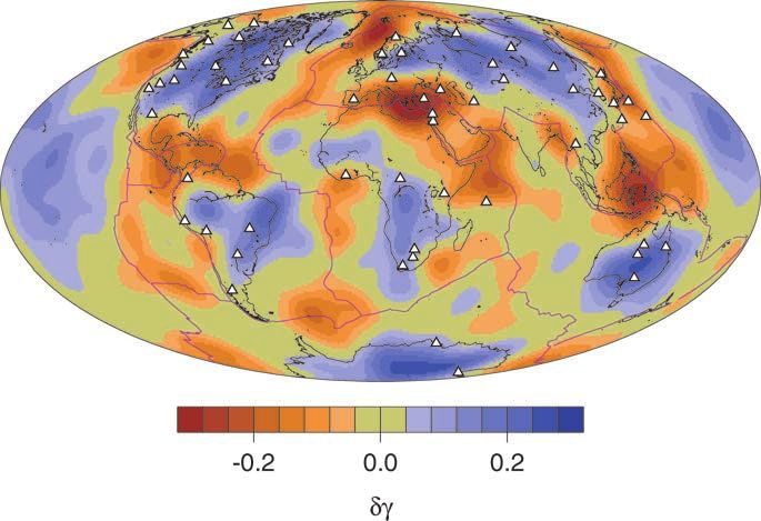
Figure 6. Distribution of δγ (θ, φ). Stations used are shown as white triangles and plate boundaries as purple lines.
where J i is the total number of stations at which event i is observed. (2) variations with period, T; and (3) a station term. So we can write:
We assume that there is a ‘true’ surface-wave magnitude, M̂ is , which
M̂ is = log10 (A/T ) + (γ + δγ p ) log10 + κ T + S j + C, (10)
is approximately equal to M is for large J i . The scatter of M isj about
M̂ is is then assumed to be due to: (1) path-dependent variation in the where δγ p is the variation in γ associated with path p, S j is the
constant γ (i.e. variations in the effect of dispersion and attenuation); station term for station j, T = (T − T 0 )/(T max − T min ), T 0 being a
C British Crown Copyright 2003/MOD, GJI, 155, 379–390Path and station corrections for M s 385
0.15
0.10
Station term / m.u. 0.05
CMAR2
PDYAR
TXAR2
KSAR2
PDAR2
PDAR3
ARCE2
ESDC2
ESDC3
MKAR
NVAR
VRAC
MSEY
TXAR
BRAR
ASAR
KSAR
MRNI
ESDC
LPAZ
CPUP
ILAR
WRA
NOA
YKA
CTA
ZAL
HIA
EIL
JHJ
JCJ
0.00
VNDA
CPUP2
ULM
SADO
MNV
NORE2
PLCA
KBZ
NRIS
ABKT
SCHQ
ARCES
BGCA2
STKA
JOW
PDY
NNA
JNU
PDAR
BDFB
MAW
NORES
BGCA
BBB
KBZ3
FINES
JKA
KBZ2
DBIC2
FRB
ROSC
DBIC
ELK
BJT
DLBC
INK
LBTB
BOSA
KMBO
NEW
SUR
CMAR
-0.05
-0.10
-0.15
Figure 7. Station corrections in magnitude units (m.u.).
reference period and κ a constant. T max and T min are the maximum Table 2. Variance reductions achieved for the M s correction model. V total
Downloaded from http://gji.oxfordjournals.org/ by guest on May 9, 2015
and minimum values of T permitted (here 22s and 18s respectively). is the variance reduction achieved for the total model, and V path , V station and
Then, assuming that Mˆsi = M is , the residual, d ij for each event- V period the variance reduction achieved by the δγ (θ , φ) distribution, station
station pair is given by corrections, and period correction respectively.
Stage V total V path V station V period
di j = M̂ is − Msi j = δγ p log10 + κ T + S j . (11)
1 26.9 16.8 8.7 1.3
We assume that we can express γ p as an integral through a 2-D 2 35.2 28.9 5.8 0.6
model expressed in spherical harmonics, i.e. 3 40.7 34.0 6.1 0.8
L
l
δγ p = xlm Yˆlm and
l=0 m=−l
Table 3. Variance reductions achieved for an alternate model in which
1
Yˆlm = Ylm (θ, φ) d(θ, φ), (12) data weights were not included, see text for details. Column headings as for
0 Table 2.
where x is the vector of model coefficients and Yˆlm is the path- Stage V total V path V station V period
average of spherical harmonics along path p. We then have a set of
1 27.9 17.7 7.6 1.3
equations of the form 2 36.8 31.5 4.7 0.8
d = Ax + By + Cz, (13) 3 41.2 35.2 5.1 1.1
where now y is a vector of station terms and z is the correction for
period. Writing
3.3 Data weighting
G= A B C (14)
We introduce an a priori data weighting scheme based on an anal-
and ysis of similar paths. The surface of the Earth is divided into
x 5◦ × 5◦ cells, with the number of paths sharing common starting and
m = y , (15) finishing squares being N s . The data weight for path p, Dp is then
z given by
this is equivalent to 1
Dp = √ . (18)
d = Gm (16) Ns
for which we find a weighted solution (Jackson 1972) of the form, The intention is to give greater weight to the contribution of unusual
paths. This is helpful because of the large variability in geographic
m = M−1 (GT G )−1 GT Dd, data coverage, which can be seen from the large variation in arrivals
where G = DGM−1 , (17) at each station (Fig. 3). The REB includes a time residual relative to
model arrival time for Rayleigh wave observations. We investigated
with D a matrix of data weights and M a matrix of model weights. the use of this time residual as an a priori measure of data quality
In practice we seek a damped solution of eq. (17) by replacing but found no correlation.
−1 −1
(G T G )−1 by UT Λ̂ U where Λ̂ = (Λ + λn I)−1 U and Λ are
the set of eigenvectors and eigenvalues of (G T G )−1 respectively,
3.4 Model weighting
and λn is the nth eigenvalue in order of size where n is cho-
sen as a compromise between model size and variance reduction Model weighting is an important issue in this type of study. First,
achieved. we impose the condition that each of the three parts of the model
C British Crown Copyright 2003/MOD, GJI, 155, 379–390386 N. D. Selby et al.
30 25
25
20
20
frequency %
frequency %
15
15
10
10
5
5
0 0
1 2 3 4 5 6 7 8 9 10 11 12 13 14 15 16 17 18 19
2 3 4 5 6 7 8
J Ms
Figure 8. Left: Histogram showing the number of observations used to calculate M s for events in the REB. For example, around 25 per cent of the events in
the REB given an M s , have that M s calculated from one observation. Right: Histogram showing the distribution of mean M s for events used in this study. Note
Downloaded from http://gji.oxfordjournals.org/ by guest on May 9, 2015
that the majority of the events have mean M s below 4.0.
[δγ (θ, φ) distribution, period dependence and set of station cor- (iii) We then recalculate residuals relative to the new mean:
rections] is weighted equally. Second, we apply a smoothness con-
di j = M is − Msi j (21)
straint to the spherical harmonic expansion of δγ (θ , φ) where each
degree, l, of the expansion is weighted by 1/[l(l + 1)]2 (Trampert and use these values in a second iteration for a degree 20 inversion.
& Woodhouse 1995). This weighting reduces the contribution of
the shorter-wavelength model components, resulting in a smoother
model. However, there is the danger that in areas of poor data- 3.6 Results
coverage and resolution the amplitude of long-wavelength structure
may be exaggerated. The resulting δγ (θ, φ) model is shown in Fig. 6(a). Paths through
A final point is that we add into the inversion the constraint blue areas give an increased value for M s whereas paths through or-
ange areas give decreased M s . There is a clear correlation with tec-
Jtot
tonic patterns, with continents and ocean basins generally enhancing
N j S j = 0, (19)
j=1
Rayleigh amplitudes and regions near plate boundaries decreasing
amplitudes. The regions of strongest negative δγ (θ, φ) occur in the
i.e. the sum of the station terms, weighted by the number of observa-
tions at each station, is equal to zero. This prevents the mean of the 1500
set of station terms trading-off with the degree zero of the spherical
harmonic expansion.
3.5 Modelling procedure
1000
(i) An initial inversion is carried out to degree 10 spherical har-
monic expansion of δγ (θ, φ) together with a set of station terms
count
and a term for period-dependence. We then calculate the misfit be-
tween observation and model prediction for each path. Paths whose
absolute misfit is greater than 2.5σ are excluded at this point.
(ii) A second inversion is carried out to degree 20. We then calcu-
500
late the model prediction for each path (station term, period term and
path term) and correct each observation. This allows us to produce
a recalculated mean for each event, M si , where:
1
Ji
M is = Mi j
Ji j=1 s
0
and Msi j = Msi j − δγ (θ, φ) − S j − κ T . (20) -0.5 -0.4 -0.3 -0.2 -0.1 0.0 0.1 0.2 0.3 0.4 0.5
δMs
This step allows for any bias in the original mean due to the path
and station corrections, i.e. we assume that M isj is closer to M̂ is than Figure 9. Histogram showing the effect of the model on mean M s for all
M isj . events given an M s during 1999.
C British Crown Copyright 2003/MOD, GJI, 155, 379–390Path and station corrections for M s 387
Figure 10. The change in M s for events during 1999. Black crosses indicate events for which the model decreases M s , i.e. the raw data overestimates M s .
Downloaded from http://gji.oxfordjournals.org/ by guest on May 9, 2015
Grey circles indicate events for which the modelling process increases M s .
Mediterranean, Indonesia and the northern Atlantic/Arctic Ocean, to record each event mean that data coverage is poor in many areas
and regions of strong positive δγ (θ , φ) are found in continental re- of the globe, both in absolute and azimuthal terms, which are equally
gions and the central Pacific. However, resolution in the southern important in this kind of study.
hemisphere (particularly in the southern Atlantic and Indian Ocean) The uneven data coverage means that the model space is not
and much of the Pacific is poor due to the scarcity of stations, the evenly sampled, which will lead to a posteriori correlations between
requirement of at least ten observations of each event, and the limit the spherical harmonic parameters. This means that ‘underdamping’
of 100◦ on path length. of the inversion could lead to spurious perturbations in the retrieved
The set of station terms range from about −0.1 to 0.15 m.u. model. Although we have attempted to minimize the effect of this
(Fig. 7). Stations with relatively few observations are likely to have problem, a more spatially complete data set is required to completely
large residuals (cf. Fig. 3) so these should be treated with caution. eliminate it. In addition, it is inevitable that some of the station terms
However, BOSA, BJT and DBIC each show large positive station will be correlated with each other and with the spherical harmonic
terms and NOA and ILAR show significant negative values. Stations coefficients. This again increases the sensitivity of the model to
CMAR, KSAR and ESDC each have multiple station terms (see correlated errors in the data.
Section 2) which can vary greatly (note in particular CMAR and However, in regions where coverage and resolution is good (North
CMAR2). This suggests that changes in instrumentation (or perhaps America, the north Atlantic and Arctic and much of Eurasia) the
changes to the total network over time) can lead to large changes models retrieved appear to be robust and revealing. If variations in
in station term, which may mean that relating station terms to local M s are due to the effects of dispersion and attenuation, then we
Earth structure is difficult. would expect to see amplitudes reduced in areas of thick sediment
Finally, we find κ = −0.05, which indicates that there is a system- or tectonic complexity. Rayleigh amplitudes should be enhanced in
atic trend of measured M s with T, with measurements made at 22s stable areas such as old continents and oceans. It is important to
being on average 0.05 m.u. lower than those made at 18s. However, remember at this point that M s is effectively a measurement of the
we also find that measurements made on continental paths are likely envelope of a seismogram convolved with a particular instrument
to be at shorter periods than those made elsewhere, so this value response or filter. M s is therefore sensitive to a range of periods
may not be independent of the δγ (θ , φ) distribution. around the measurement period determined by the dispersion (group
Table 2 lists the variance reductions achieved for each stage of the speed curve), amplitude spectrum and filter or instrument response.
modelling process and the variance reduction due to each part of the We should not necessarily expect the resulting model to correlate
model. Note that since the model parameters are not orthogonal, with existing studies of phase-speed or attenuation.
there is no requirement that V total = V path + V station + V period . In
Table 3 we list the equivalent variance reductions for an alternate
set of models where we included no data weighting. The variance
4.1 Regional biases in Ms
reductions achieved are similar.
Using our model of path, station and period corrections it is now
possible to investigate whether there are systematic regional biases
in the estimation of M s . To test this we use the set of events reported
4 DISCUSSION
during 1999 which are given an M s value in the REB, subject to
Currently the IMS network is probably insufficient to recover a fully the same data-editing as described above. The model described was
accurate model for M s corrections. The sparse station network in the constructed using only events for which J i ≥ 10 where J i is the
southern hemisphere and Pacific region together with the restriction number of stations observing event i. However, this is only a small
of path length ≤ 100◦ and the requirement for at least 10 stations sub-set of the events with surface wave magnitude given in the REB.
C British Crown Copyright 2003/MOD, GJI, 155, 379–390388 N. D. Selby et al.
Downloaded from http://gji.oxfordjournals.org/ by guest on May 9, 2015
Figure 11. The effect of the modelling process on M s residuals observed at station NOA, Norway. Top: Observed M s residuals. Middle: Model predicted
residuals. Bottom: Difference between observed and predicted residuals. Distinct clusters of positive and negative residuals are still visible.
Fig. 8 shows the distribution of J i for 1999. More than 25 per cent is smaller than the original. We see that the original M s was overes-
of the events with an M s have that magnitude calculated from only timated in regions such as central Asia, the western margin of North
one observation. and South America, Japan and the Tonga-Kermadec trench region.
We calculate the M s correction for each observation in the REB The grey circles show that events in the eastern Mediterranean and
and then recalculate M is for all i. Fig. 9 shows the difference between Middle East as well as those in Indonesia are underestimated if the
the original and updated mean M s (negative values indicate that corrections are not used.
the original M is is an underestimate). Most of these differences are
between ±0.2.
4.2 Possible effect of data censoring
We then investigate the geographic distribution of M s bias. In
Fig. 10 we show the distribution of events for which the |M is − M is | > Surface wave observations are required to pass a dispersion test
0.1. Black crosses indicate events for which the revised magnitude before M s can be reported in the REB (Stevens & McLaughlin
C British Crown Copyright 2003/MOD, GJI, 155, 379–390Path and station corrections for M s 389
2001). This means that any surface waves which deviate greatly derstanding of M s residual distribution across the Earth can only
from the model group speed predictions will not be included. If, as improve.
we assume, M s residuals are at least partly related to the shape of This paper does not discuss the relationship between M s and M 0 ,
the group-speed curve for a path, then the observations of amplitude which has been discussed elsewhere (e.g. Ekström & Dziewonski
are not independent of the group-speed model, i.e. amplitudes will 1988; Herak et al. 2001). We also do not discuss the relationship
not be measured for paths which do not fit the group-speed model, between M s and the yield of explosions (e.g. Marshall et al. 1971;
producing a data-censoring effect. However, we feel that this is a Stevens & Murphy 2001). However, the results presented here sug-
weak effect since the time window used in association with the gest further work which may improve our understanding of these
group-speed curves is wide enough to allow any genuine surface relationships.
wave to be detected. The censoring effect is certainly not comparable A final word of caution is that the results in this study can only be
to that in any study which utilizes a waveform-fitting technique of guaranteed to apply to M s measurements made using the method-
surface-wave measurement. ology of Stevens & McLaughlin (2001) described above. Surface
waves generated from small, shallow explosions have a different
character to earthquake data (having a much higher frequency con-
4.3 Remaining residuals
tent) and so may require a more appropriate method of M s measure-
The modelling process above accounts for around 40 per cent of the ment (such as that described by Marshall & Basham 1972) which
variance of the observations, and so a large part of the observations would require frequency-dependent path and station corrections.
are not explained by the model. In Fig. 11 we show the effect of the
modelling on the observed station residuals. The top panel shows
AC K N OW L E D G M E N T S
the observed residuals for station NOA in southern Norway, plotted
in the same way as Fig. 5. In the middle panel are the model pre- The figures in this paper were produced using GMT (Wessel & Smith
Downloaded from http://gji.oxfordjournals.org/ by guest on May 9, 2015
dictions. Although the general pattern of the predictions matches 1998). The authors would like to thank the staff of the pIDC, IDC
the observations, the size of the residuals is generally smaller. This and IMS responsible for producing the data utilized here.
is presumably because of the trade-off with observations at other
stations. The bottom panel shows what remains of the observations
after modelling. there are still distinct patterns of residuals, particu- REFERENCES
larly in the western Pacific and Atlantic regions. These residuals are
Båth, M., 1952. Earthquake magnitude determination from the vertical com-
not explainable within the framework outlined above. We surmise ponent of surface waves, Trans. Amer. geop. Un., 33, 81–90.
that these residuals are due either to path effects which cannot be pre- Båth, M., 1981. Earthquake magnitude—recent research and current trends,
dicted by our model—for instance, there may be systematic effects Earthquake Sci. Rev., 17, 315–398.
on amplitude dependent on the angle of intersection between the Billien, M., Lévêque, J.-J. & Trampert, J., 2000. Global maps of Rayleigh
path and an ocean/continent boundary—or to the effects of source wave attenuation for periods between 40 and 150 seconds, Geophys. Res.
radiation pattern. However, preliminary attempts to match radia- Lett., 27, 3619–3622.
tion patterns from earthquakes with known mechanisms to either Boore, D.M. & Toksöz, N., 1969. Rayleigh-wave particle motion and crustal
the initial observations or the residuals after modelling have proved structure, Bull. seism. Soc. Am., 59, 331–346.
inconclusive, so this question remains to be resolved. Bowers, D., 1997. The October 30, 1994, seismic disturbance in South Africa:
earthquake or large rock burst?, J. geophys. Res, 102, 9843–9857.
Bowers, D. & Douglas, A., 1998. The effect of the earthquake radiation
5 C O N C LU S I O N S pattern on mb —a study using aftershocks in the 1976 Gazli sequence,
Bull. seism. Soc. Am., 88, 523–530.
M s residuals show systematic patterns which can, at least in part, be Bowers, D. & McCormack, D.A., 1997. The mechanisms of shallow earth-
attributed to lateral variations in Earth structure. Determining reli- quakes and the monitoring of a comprehensive test ban, Geophys. J. Int.,
able M s path corrections is potentially vital since event screening 128, 701–707.
and discrimination can depend critically on the use of the mb : M s Carpenter, E.W. & Marshall, P.D., 1970. Surface waves generated by atmo-
criterion. If the number of M s observations is very low, which is spheric nuclear explosions., AWRE Report, O 88/70, United Kingdom
likely to be so for small explosions, then path and station dependent Atomic Energy Authority, H.M.S.O.
effects can potentially bias the observed M s of a seismic distur- Ekström, G. & Dziewonski, A.M., 1988. Evidence of bias in estimations of
earthquake size, Nature, 332, 319–323.
bance. However, it is critical that any postulated M s corrections are
Ewing, W.M., Jardetzky, W.S. & Press, F., 1957. Elastic Waves in Layered
not contaminated by earthquake radiation pattern effects since these Media, McGraw-Hill, New York, USA.
would not be applicable to explosions. Hence, using the raw data, Gutenberg, B., 1945. Amplitudes of surface waves and magnitudes of shal-
‘source-station specific’ type corrections will probably be contami- low earthquakes, Bull. seism. Soc. Am., 35, 3–12.
nated more by radiation pattern effects than this type of model. Also, Herak, M., Panza, G.F. & Costa, G., 2001. Theoretical and observed depth
station corrections for M s need to be de-sensitized to the effects of correction for M s , Pure appl. Geophys., 158, 1517–1530.
path-dependent variations in M s , so that they can be applied with Jackson, D.D., 1972. Interpretation of inaccurate, insufficient and inconsis-
equal validity to events happening in any region of the Earth. A joint tent data, Geophys. J.R. astr. Soc., 28, 97–109.
inversion such as is described here can go some way to achieving Kanamori, H., 1977. The energy release in great earthquakes, J. geophys.
this. Res, 82, 2981–2987.
Marshall, P.D. & Basham, P.W., 1972. Discrimination between earthquakes
The type of results presented here are potentially beneficial in
and explosions employing an improved M s scale, Geophys. J. R. astr. Soc.,
studies of Earth structure, and complementary to group-speed stud- 28, 431–458.
ies using Rayleigh waves of similar periods (see, for example Marshall, P.D., Douglas, A. & Hudson, J.A., 1971. Surface waves from un-
Ritzwoller & Levshin 1998; Vdovin et al. 1999). As the IMS net- derground explosions, Nature, 234, 8–9.
work grows, and if, as has been suggested, greater efforts are made Rezapour, M. & Pearce, R.G., 1998. Bias in surface-wave magnitude M s
to retrieve long-period data from IMS auxiliary stations, our un- due to inadequate distance corrections, Bull. seism. Soc. Am., 88, 43–61.
C British Crown Copyright 2003/MOD, GJI, 155, 379–390390 N. D. Selby et al.
Richter, C.F., 1958. Elementary Seismology, W. H. Freeman and Company, Thomas, J.H., Marshall, P.D. & Douglas, A., 1978. Rayleigh wave amplitudes
San Francisco, USA. from earthquakes in the range 0◦ to 150◦ , Geophys. J. R. astr. Soc, 53,
Ritzwoller, M.H. & Levshin, A.L., 1998. Eurasian surface wave tomography: 191–200.
group velocities, J. geophys. Res., 103, 4839–4878. Trampert, J. & Woodhouse, J.H., 1995. Global phase velocity maps of Love
Selby, N.D. & Woodhouse, J.H., 2000. Controls on Rayleigh wave ampli- and Rayleigh waves between 40 and 150 seconds, Geophys. J. Int., 122,
tudes: attenuation and focusing, Geophys. J. Int., 142, 933–940. 675–690.
Sexton, J.L., Rudman, A.J. & Mead, J., 1977. Ellipticity of Rayleigh waves Vdovin, O., Rial, J.A., Levshin, A. & Ritzwoller, M.H., 1999. Group-velocity
recorded in the Midwest, Bull. seism. Soc. Am., 67, 369–382. tomography of South America and the surrounding oceans, Geophys. J.
Stevens, J.L. & McLaughlin, K.L., 2001. Optimization of surface wave Int., 136, 324–340.
identification and measurement, Pure Appl. Geophys., 158, 1547– von Seggern, D.H., 1970. The effects of radiation pattern on magnitude
1582. estimates, Bull. seism. Soc. Am., 60, 503–516.
Stevens, J.L. & Murphy, J.R., 2001. Yield estimation from surface-wave Wessel, P. & Smith, W.H.F., 1998. New, improved version of the Generic
amplitudes, Pure Appl. Geophys., 158, 2227–2252. Mapping Tools released, EOS, Trans. Am. geophys. Un., 79, 579.
Downloaded from http://gji.oxfordjournals.org/ by guest on May 9, 2015
C British Crown Copyright 2003/MOD, GJI, 155, 379–390You can also read


