Lifelong Multi-Agent Path Finding in Large-Scale Warehouses
←
→
Page content transcription
If your browser does not render page correctly, please read the page content below
Lifelong Multi-Agent Path Finding in Large-Scale Warehouses*
                                                                             Jiaoyang Li,1 Andrew Tinka,2 Scott Kiesel,2
                                                                       Joseph W. Durham,2 T. K. Satish Kumar,1 Sven Koenig1
                                                                                           1
                                                                                         University of Southern California
                                                                                               2
                                                                                                 Amazon Robotics
                                                     jiaoyanl@usc.edu, {atinka, skkiesel, josepdur}@amazon.com, tkskwork@gmail.com, skoenig@usc.edu
arXiv:2005.07371v2 [cs.AI] 12 Mar 2021

                                                                    Abstract                                     Existing methods for solving lifelong MAPF include (1)
                                                                                                              solving it as a whole (Nguyen et al. 2017), (2) decompos-
                                           Multi-Agent Path Finding (MAPF) is the problem of mov-             ing it into a sequence of MAPF instances where one re-
                                           ing a team of agents to their goal locations without colli-
                                           sions. In this paper, we study the lifelong variant of MAPF,
                                                                                                              plans paths at every timestep for all agents (Wan et al. 2018;
                                           where agents are constantly engaged with new goal loca-            Grenouilleau, van Hoeve, and Hooker 2019), and (3) de-
                                           tions, such as in large-scale automated warehouses. We pro-        composing it into a sequence of MAPF instances where one
                                           pose a new framework Rolling-Horizon Collision Resolu-             plans new paths at every timestep for only the agents with
                                           tion (RHCR) for solving lifelong MAPF by decomposing               new goal locations (Cáp, Vokrı́nek, and Kleiner 2015; Ma
                                           the problem into a sequence of Windowed MAPF instances,            et al. 2017; Liu et al. 2019).
                                           where a Windowed MAPF solver resolves collisions among                In this paper, we propose a new framework Rolling-
                                           the paths of the agents only within a bounded time horizon         Horizon Collision Resolution (RHCR) for solving lifelong
                                           and ignores collisions beyond it. RHCR is particularly well        MAPF where we decompose lifelong MAPF into a sequence
                                           suited to generating pliable plans that adapt to continually       of Windowed MAPF instances and replan paths once every
                                           arriving new goal locations. We empirically evaluate RHCR
                                           with a variety of MAPF solvers and show that it can produce
                                                                                                              h timesteps (replanning period h is user-specified) for in-
                                           high-quality solutions for up to 1,000 agents (= 38.9% of the      terleaving planning and execution. A Windowed MAPF in-
                                           empty cells on the map) for simulated warehouse instances,         stance is different from a regular MAPF instance in the fol-
                                           significantly outperforming existing work.                         lowing ways:
                                                                                                             1. it allows an agent to be assigned a sequence of goal loca-
                                                              1    Introduction                                  tions within the same Windowed MAPF episode, and
                                         Multi-Agent Path Finding (MAPF) is the problem of mov-              2. collisions need to be resolved only for the first w
                                         ing a team of agents from their start locations to their goal           timesteps (time horizon w ≥ h is user-specified).
                                         locations while avoiding collisions. The quality of a solution       The benefit of this decomposition is two-fold. First, it keeps
                                         is measured by flowtime (the sum of the arrival times of all         the agents continually engaged, avoiding idle time, and thus
                                         agents at their goal locations) or makespan (the maximum of          increasing throughput. Second, it generates pliable plans that
                                         the arrival times of all agents at their goal locations). MAPF       adapt to continually arriving new goal locations. In fact, re-
                                         is NP-hard to solve optimally (Yu and LaValle 2013).                 solving collisions in the entire time horizon (i.e., w = ∞) is
                                            MAPF has numerous real-world applications, such as                often unnecessary since the paths of the agents can change
                                         autonomous aircraft-towing vehicles (Morris et al. 2016),            as new goal locations arrive.
                                         video game characters (Li et al. 2020b), and quadro-                    We evaluate RHCR with various MAPF solvers, namely
                                         tor swarms (Hönig et al. 2018). Today, in automated                 CA* (Silver 2005) (incomplete and suboptimal), PBS (Ma
                                         warehouses, mobile robots called drive units already au-             et al. 2019) (incomplete and suboptimal), ECBS (Barer
                                         tonomously move inventory pods or flat packages from one             et al. 2014) (complete and bounded suboptimal), and
                                         location to another (Wurman, D’Andrea, and Mountz 2007;              CBS (Sharon et al. 2015) (complete and optimal). We show
                                         Kou et al. 2020). However, MAPF is only the “one-shot”               that, for each MAPF solver, using a bounded time horizon
                                         variant of the actual problem in many applications. Typi-            yields similar throughput as using the entire time horizon
                                         cally, after an agent reaches its goal location, it does not stop    but with a significantly smaller runtime. We also show that
                                         and wait there forever. Instead, it is assigned a new goal lo-       RHCR outperforms existing work and can scale up to 1,000
                                         cation and required to keep moving, which is referred to as          agents (= 38.9% of the empty cells on the map) for simulated
                                         lifelong MAPF (Ma et al. 2017) and characterized by agents           warehouse instances.
                                         constantly being assigned new goal locations.
                                            * This paper is an extension of (Li et al. 2020c).
                                                                                                                                  2   Background
                                         Copyright © 2021, Association for the Advancement of Artificial      In this section, we first introduce several state-of-the-art
                                         Intelligence (www.aaai.org). All rights reserved.                   MAPF solvers and then discuss existing research on life-
long MAPF. We finally review the elements of the bounded
horizon idea that have guided previous research.
2.1 Popular MAPF Solvers
Many MAPF solvers have been proposed in recent years,
including rule-based solvers (Luna and Bekris 2011;
de Wilde, ter Mors, and Witteveen 2013), prioritized plan-
ning (Okumura et al. 2019), compilation-based solvers (Lam
et al. 2019; Surynek 2019), A*-based solvers (Golden- (a) Fulfillment warehouse map, borrowed from (Wurman,
berg et al. 2014; Wagner 2015), and dedicated search-based D’Andrea, and Mountz 2007).
solvers (Sharon et al. 2013; Barer et al. 2014). We present
four representative MAPF solvers.
CBS Conflict-Based Search (CBS) (Sharon et al. 2015) is
a popular two-level MAPF solver that is complete and opti-
mal. At the high level, CBS starts with a root node that con-
tains a shortest path for each agent (ignoring other agents).
It then chooses and resolves a collision by generating two
child nodes, each with an additional constraint that prohibits
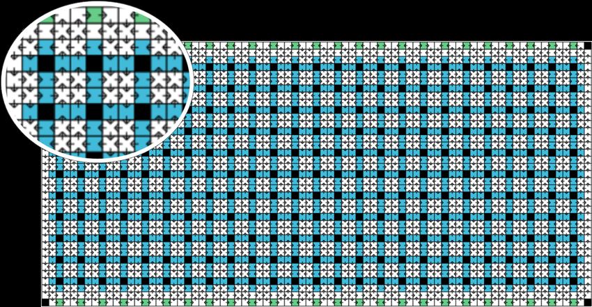
one of the agents involved in the collision from being at the (b) Sorting center map, modified from (Wan et al. 2018).
colliding location at the colliding timestep. It then calls its
low level to replan the paths of the agents with the new con- Figure 1: A well-formed fulfillment warehouse map and a
straints. CBS repeats this procedure until it finds a node with non-well-formed sorting center map. Orange squares repre-
collision-free paths. CBS and its enhanced variants (Gange, sent robots. In (a), the endpoints consist of the green cells
Harabor, and Stuckey 2019; Li et al. 2019, 2020a) are among (representing locations that store inventory pods) and blue
the state-of-the-art optimal MAPF solvers. cells (representing the work stations). In (b), the endpoints
consist of the blue cells (representing locations where the
drive units drop off packages) and pink cells (represent-
ECBS Enhanced CBS (ECBS) (Barer et al. 2014) is a
ing the loading stations). Black cells labeled “X” represent
complete and bounded-suboptimal variant of CBS. The
chutes (obstacles).
bounded suboptimality (i.e., the solution cost is a user-
specified factor away from the optimal cost) is achieved
by using focal search (Pearl and Kim 1982), instead of
best-first search, in both the high- and low-level searches 2.2 Prior Work on Lifelong MAPF
of CBS. ECBS is the state-of-the-art bounded-suboptimal We classify prior work on lifelong MAPF into three cate-
MAPF solver. gories.
CA* Cooperative A* (CA*) (Silver 2005) is based on a Method (1) The first method is to solve lifelong MAPF as
simple prioritized-planning scheme: Each agent is given a a whole in an offline setting (i.e., knowing all goal locations
unique priority and computes, in priority order, a shortest a priori) by reducing lifelong MAPF to other well-studied
path that does not collide with the (already planned) paths of problems. For example, Nguyen et al. (2017) formulate life-
agents with higher priorities. CA*, or prioritized planning in long MAPF as an answer set programming problem. How-
general, is widely used in practice due to its small runtime. ever, the method only scales up to 20 agents in their paper,
However, it is suboptimal and incomplete since its prede- each with only about 4 goal locations. This is not surpris-
fined priority ordering can sometimes result in solutions of ing because MAPF is a challenging problem and its lifelong
bad quality or even fail to find any solutions for solvable variant is even harder.
MAPF instances.
Method (2) A second method is to decompose lifelong
PBS Priority-Based Search (PBS) (Ma et al. 2019) com- MAPF into a sequence of MAPF instances where one re-
bines the ideas of CBS and CA*. The high level of PBS is plans paths at every timestep for all agents. To improve the
similar to CBS except that, when resolving a collision, in- scalability, researchers have developed incremental search
stead of adding additional constraints to the resulting child techniques that reuse previous search effort. For example,
nodes, PBS assigns one of the agents involved in the colli- Wan et al. (2018) propose an incremental variant of CBS that
sion a higher priority than the other agent in the child nodes. reuses the tree of the previous high-level search. However,
The low level of PBS is similar to CA* in that it plans a it has substantial overhead in constructing a new high-level
shortest path that is consistent with the partial priority or- tree from the previous one and thus does not improve the
dering generated by the high level. PBS outperforms many scalability by much. Svancara et al. (2019) use the frame-
variants of prioritized planning in terms of solution quality work of Independence Detection (Standley 2010) to reuse
but is still incomplete and suboptimal. the paths from the previous iteration. It replans paths foronly the new agents (in our case, agents with new goal loca- 3 Problem Definition
tions) and the agents whose paths are affected by the paths
The input is a graph G = (V, E), whose vertices V corre-
of the new agents. However, when the environment is dense
spond to locations and whose edges E correspond to con-
(i.e., contains many agents and many obstacles, which is
nections between two neighboring locations, and a set of m
common for warehouse scenarios), almost all paths are af-
agents {a1 , . . . , am }, each with an initial location. We study
fected, and thus it still needs to replan paths for most agents.
an online setting where we do not know all goal locations
a priori. We assume that there is a task assigner (outside of
Method (3) A third method is similar to the second our path-planning system) that the agents can request goal
method but restricts replanning to the paths of the agents locations from during the operation of the system.1 Time is
that have just reached their goal locations. The new paths discretized into timesteps. At each timestep, every agent can
need to avoid collisions not only with each other but also either move to a neighboring location or wait at its current
with the paths of the other agents. Hence, this method could location. Both move and wait actions have unit duration. A
degenerate to prioritized planning in case where only one collision occurs iff two agents occupy the same location at
agent reaches its goal location at every timestep. As a result, the same timestep (called a vertex conflict in (Stern et al.
the general drawbacks of prioritized planning, namely its in- 2019)) or traverse the same edge in opposite directions at
completeness and its potential to generate costly solutions, the same timestep (called a swapping conflict in (Stern et al.
resurface in this method. To address the incompleteness is- 2019)). Our task is to plan collision-free paths that move
sue, Cáp, Vokrı́nek, and Kleiner (2015) introduce the idea of all agents to their goal locations and maximize the through-
well-formed infrastructures to enable backtrack-free search. put, i.e., the average number of goal locations visited per
In well-formed infrastructures, all possible goal locations timestep. We refer to the set of collision-free paths for all
are regarded as endpoints, and, for every pair of endpoints, agents as a MAPF plan.
there exists a path that connects them without traversing any We study the case where the task assigner is not within our
other endpoints. In real-world applications, some maps, such control so that our path-planning system is applicable in dif-
as the one in Figure 1a, may satisfy this requirement, but ferent domains. But, for a particular domain, one can design
other maps, such as the one in Figure 1b, may not. More- a hierarchical framework that combines a domain-specific
over, additional mechanisms are required during path plan- task assigner with our domain-independent path-planning
ning. For example, one needs to force the agents to “hold” system. Compared to coupled methods that solve task as-
their goal locations (Ma et al. 2017) or plan “dummy paths” signment and path finding jointly, a hierarchical framework
for the agents (Liu et al. 2019) after they reach their goal lo- is usually a good way to achieve efficiency. For example, the
cations. Both alternatives result in unnecessarily long paths task assigners in (Ma et al. 2017; Liu et al. 2019) for fulfill-
for agents, decreasing the overall throughput, as shown in ment warehouse applications and in (Grenouilleau, van Ho-
our experiments. eve, and Hooker 2019) for sorting center applications can be
directly combined with our path-planning system. We also
Summary Method (1) needs to know all goal locations a showcase two simple task assigners, one for each applica-
priori and has limited scalability. Method (2) can work in tion, in our experiments.
an online setting and scales better than Method (1). How- We assume that the drive units can execute any MAPF
ever, replanning for all agents at every timestep is time- plan perfectly. Although this seems to be not realistic, there
consuming even if one uses incremental search techniques. exist some post-processing methods (Hönig et al. 2016) that
As a result, its scalability is also limited. Method (3) scales can take the kinematic constraints of drive units into consid-
to substantially more agents than the first two methods, but eration and convert MAPF plans to executable commands
the map needs to have an additional structure to guarantee for them that result in robust execution. For example, Hönig
completeness. As a result, it works only for specific classes et al. (2019) propose a framework that interleaves planning
of lifelong MAPF instances. In addition, Methods (2) and and execution and can be directly incorporated with our
(3) plan at every timestep, which may not be practical since framework RHCR.
planning is time-consuming.
4 Rolling-Horizon Collision Resolution
2.3 Bounded-Horizon Planing
Rolling-Horizon Collision Resolution (RHCR) has two
Bounded-horizon planning is not a new idea. Silver (2005) user-specified parameters, namely the time horizon w and
has already applied this idea to regular MAPF with CA*. the replanning period h. The time horizon w specifies that
He refers to it as Windowed Hierarchical Cooperative A* the Windowed MAPF solver has to resolve collisions within
(WHCA*) and empirically shows that WHCA* runs faster a time horizon of w timesteps. The replanning period h spec-
as the length of the bounded horizon decreases but also gen- ifies that the Windowed MAPF solver needs to replan paths
erates longer paths. In this paper, we showcase the benefits once every h timesteps. The Windowed MAPF solver has to
of applying this idea to lifelong MAPF and other MAPF
solvers. In particular, RHCR yields the benefits of lower 1
In case there are only a finite number of tasks, after all tasks
computational costs for planning with bounded horizons have been assigned, we assume that the task assigner will assign
while keeping the agents busy and yet, unlike WHCA* for a dummy task to an agent whose goal location is, e.g., a charging
regular MAPF, decreasing the solution quality only slightly. station, an exit, or the current location of the agent.replan paths more frequently than once every w timesteps to Algorithm 1: The low-level search for Win-
avoid collisions, i.e., w should be larger than or equal to h. dowed MAPF solvers generalizing Multi-Label
In every Windowed MAPF episode, say, starting at A* (Grenouilleau, van Hoeve, and Hooker 2019).
timestep t, RHCR first updates the start location si and the Input: Start location si , goal location sequence gi .
goal location sequence gi for each agent ai . RHCR sets the
start location si of agent ai to its location at timestep t. Then, 1 R.location ← si , R.time ← 0, R.g ← 0;
RHCR calculates a lower bound on the number of timesteps 2 R.label ← 0;
d that agent ai needs to visit all remaining locations in gi , 3 R.h ← C OMPUTE HVALUE(R.location, R.label );
i.e., 4 open.push(R);
5 while open is not empty do
|gi |−1
X 6 P ← open.pop(); // Pop the node with the
d = dist(si , gi [0]) + dist(gi [j − 1], gi [j]), (1) minimum f .
j=1 7 if P.location = gi [P.label ] then // Update label.
8 P.label ← P.label + 1;
where dist(x, y) is the distance from location x to location y
and |x| is the cardinality in sequence x.2 d being smaller 9 if P.label = |gi | then // Goal test.
than h indicates that agent ai might finish visiting all its 10 return the path retrieved from P ;
goal locations and then being idle before the next Windowed 11 foreach child node Q of P do // Generate child
MAPF episode starts at timestep t + h. To avoid this situa- nodes.
tion, RHCR continually assigns new goal locations to agent 12 open.push(Q);
ai until d ≥ h. Once the start locations and the goal location
sequences for all agents require no more updates, RHCR 13 return “No Solution”;
calls a Windowed MAPF solver to find paths for all agents 14 Function C OMPUTE HVALUE(Location x, Label l) :
that move them from their start locations to all their goal lo- 15 return
cations in the order given by their goal location sequences P|gi |−1
and are collision-free for the first w timesteps. Finally, it dist(x , gi [l ]) + j=l+1 dist(gi [j − 1], gi [j]);
moves the agents for h timesteps along the generated paths
and remove the visited goal locations from their goal loca-
tion sequences.
RHCR uses flowtime as the objective of the Windowed of regular MAPF solvers can be adapted to the low-level
MAPF solver, which is known to be a reasonable objective search of Windowed MAPF solvers. In fact, Grenouilleau,
for lifelong MAPF (Svancara et al. 2019). Compared to reg- van Hoeve, and Hooker (2019) perform a truncated version
ular MAPF solvers, Windowed MAPF solvers need to be of this adaptation for the pickup and delivery problem. They
changed in two aspects: propose Multi-Label A* that can find a path for a single
agent that visits two ordered goal locations, namely its as-
1. each path needs to visit a sequence of goal locations, and signed pickup location and its goal location. In Algorithm 1,
2. the paths need to be collision-free for only the first w we generalize Multi-Label A* to a sequence of goal loca-
timesteps. tions.3
We describe these changes in detail in the following two sub- Algorithm 1 uses the structure of location-time A*. For
sections. each node N , we add an additional attribute N.label that
indicates the number of goal locations in the goal location
4.1 A* for a Goal Location Sequence sequence gi that the path from the root node to node N has
already visited. For example, N.label = 2 indicates that the
The low-level searches of all MAPF solvers discussed in path has already visited goal locations gi [0] and gi [1] but
Section 2.1 need to find a path for an agent from its start not goal location gi [2]. Algorithm 1 computes the h-value
location to its goal location while satisfying given spatio- of a node as the distance from the location of the node to the
temporal constraints that prohibit the agent from being at next goal location plus the sum of the distances between con-
certain locations at certain timesteps. Therefore, they often secutive future goal locations in the goal location sequence
use location-time A* (Silver 2005) (i.e., A* that searches in [Lines 14-15]. In the main procedure, Algorithm 1 first cre-
the location-time space where each state is a pair of location ates the root node R with label 0 and pushes it into the pri-
and timestep) or any of its variants. However, a characteris-
tic feature of a Windowed MAPF solver is that it plans a path 3
Planning a path for an agent to visit a sequence of goal lo-
for each agent that visits a sequence of goal locations. De- cations is not straightforward. While one can call a sequence of
spite this difference, techniques used in the low-level search location-time A* to plan a shortest path between every two con-
secutive goal locations and concatenate the resulting paths, the
2
Computing d relies on the distance function dist(x, y). Here, overall path is not necessarily the shortest because the presence
and in any other place where dist(x, y) is required, prepossessing of spatio-temporal constraints introduces spatio-temporal depen-
techniques can be used to increase efficiency. In particular, large dencies among the path segments between different goal locations,
warehouses have a candidate set of goal locations as the only pos- e.g., arriving at the first goal location at the earliest timestep may
sible values for y, enabling the pre-computation and caching of result in a longer overall path than arriving there later. We therefore
shortest-path trees. need Algorithm 1.oritized queue open [Lines 1-4]. While open is not empty bounded-horizon PBS generates smaller high-level trees and
[Line 5], the node P with the smallest f -value is selected runs faster in its low level than standard PBS.
for expansion [Line 6]. If P has reached its current goal lo-
cation [Line 7], P.label is incremented [Line 8]. If P.label 4.3 Behavior of RHCR
equals the cardinality of the goal location sequence [Line 9], We first show that resolving collisions for a longer time hori-
Algorithm 1 terminates and returns the path [Line 10]. Oth- zon in lifelong MAPF does not necessarily result in better
erwise, it generates child nodes that respect the given spatio- solutions. Below is such an example.
temporal constraints [Lines 11-12]. The labels of the child Example 1. Consider the lifelong MAPF instance shown
nodes equal P.label . Checking the priority queue for dupli- in Figure 2a with time horizon w = 4 and replanning pe-
cates requires a comparison of labels in addition to other riod h = 2, and assume that we use an optimal Windowed
attributes. MAPF solver. At timestep 0 (left figure), all agents follow
their shortest paths as no collisions will occur during the
4.2 Bounded-Horizon MAPF Solvers first 4 timesteps. Then, agent a3 reaches its goal location at
Another characteristic feature of Windowed MAPF solvers timestep 2 and is assigned a new goal location (right figure).
is the use of a bounded horizon. Regular MAPF solvers can If agents a1 and a3 both follow their shortest paths, the Win-
be easily adapted to resolving collisions for only the first w dowed MAPF solver finds a collision between them at cell B
timesteps. Beyond the first w timesteps, the solvers ignore at timestep 3 and forces agent a1 to wait for one timestep.
collisions among agents and assume that each agent follows The resulting number of wait actions is 1. However, if we
its shortest path to visit all its goal locations, which ensures solve this example with time horizon w = 8, as shown in
that the agents head in the correct directions in most cases. Figure 2b, we could generate paths with more wait actions.
We now provide details on how to modify the various MAPF At timestep 0 (left figure), the Windowed MAPF solver finds
solvers discussed in Section 2.1. a collision between agents a1 and a2 at cell A at timestep 6
and thus forces agent a2 to wait for one timestep. Then, at
timestep 2 (right figure), the Windowed MAPF solver finds
Bounded-Horizon (E)CBS Both CBS and ECBS search a collision between agents a1 and a3 at cell B at timestep 3
by detecting and resolving collisions. In their bounded- and forces agent a3 to wait for one timestep. The resulting
horizon variants, we only need to modify the collision detec- number of wait actions is 2.
tion function. While (E)CBS finds collisions among all paths
and can then resolve any one of them, bounded-horizon Similar cases are also found in our experiments: some-
(E)CBS only finds collisions among all paths that occur times RHCR with smaller time horizons achieves higher
in the first w timesteps and can then resolve any one of throughput than with larger time horizons. All of these cases
them. The remaining parts of (E)CBS stay the same. Since support our claim that, in lifelong MAPF, resolving all col-
bounded-horizon (E)CBS needs to resolve fewer collisions, lisions in the entire time horizon is unnecessary, which is
it generates a smaller high-level tree and thus runs faster than different from regular MAPF. Nevertheless, the bounded-
standard (E)CBS. horizon method also has a drawback since using too small
a value for the time horizon may generate deadlocks that
prevent agents from reaching their goal locations, as shown
Bounded-Horizon CA* CA* searches based on prior- in Example 2.
ities, where an agent avoids collisions with all higher- Example 2. Consider the lifelong MAPF instance shown
priority agents. In its bounded-horizon variant, an agent is in Figure 2c with time horizon w = 2 and replanning pe-
required to avoid collisions with all higher-priority agents riod h = 2, and assume that we use an optimal Windowed
but only during the first w timesteps. Therefore, when run- MAPF solver. At timestep 0, the Windowed MAPF solver re-
ning location-time A* for each agent, we only consider the turns path [B, B, B, C, D, E] (of length 5) for agent a1 and
spatio-temporal constraints during the first w timesteps in- path [C, C, C, B, A, L] (of length 5) for agent a2 , which are
duced by the paths of higher-priority agents. The remaining collision-free for the first 2 timesteps. It does not return the
parts of CA* stay the same. Since bounded-horizon CA* has collision-free paths where one of the agents uses the upper
fewer spatio-temporal constraints, it runs faster and is less corridor, nor the collision-free paths where one of the agents
likely to fail to find solutions than CA*. Bounded-horizon leaves the lower corridor first (to let the other agent reach
CA* is identical to WHCA* in (Silver 2005). its goal location) and then re-enters it, because the resulting
flowtime is larger than 5 + 5 = 10. Therefore, at timestep 2,
Bounded-Horizon PBS The high-level search of PBS is both agents are still waiting at cells B and C. The Windowed
similar to that of CBS and is based on resolving collisions, MAPF solver then finds the same paths for both agents again
while the low-level search of PBS is similar to that of CA* and forces them to wait for two more timesteps. Overall, the
and plans paths that are consistent with the partial prior- agents wait at cells B and C forever and never reach their
ity ordering generated by the high-level search. Hence, we goal locations.
need to modify the collision detection function of the high
level of PBS (just like how we modify CBS) and incorpo- 4.4 Avoiding Deadlocks
rate the limited consideration of spatio-temporal constraints To address the deadlock issue shown in Example 2, we can
into its low level (just like how we modify CA*). As a result, design a potential function to evaluate the progress of the(a) A lifelong MAPF instance with time horizon w = (b) The same lifelong MAPF instance as shown in (a) (c) A lifelong MAPF
4. Agent a3 reaches its goal location at timestep 2 and with time horizon w = 8. instance with time
is then assigned a new goal location. horizon w = 2.
Figure 2: Lifelong MAPF instances with replanning period h = 2. Solid (dashed) circles represent the current (goal) locations
of the agents.
agents and increase the time horizon if the agents do not
make sufficient progress. For example, after the Windowed
MAPF solver returns a set of paths, we compute the po-
tential function P (w) = |{ai |C OMPUTE HVALUE(xi , li ) <
C OMPUTE HVALUE(si , 0), 1 ≤ i ≤ m}|, where function
C OMPUTE HVALUE(·, ·) is defined on Lines 14-15 in Algo-
rithm 1, xi is the location of agent ai at timestep w, li is
the number of goal locations that it has visited during the
first w timesteps, and si is its location at timestep 0. P (w)
estimates the number of agents that need fewer timesteps to (a) Fulfillment warehouse map.
visit all their goal locations from timestep w on than from
timestep 0 on. We increase w and continue running the Win-
dowed MAPF solver until P (w) ≥ p, where p ∈ [0, m] is a
user-specified parameter. This ensures that at least p agents
have visited (some of) their goal locations or got closer to
their next goal locations during the first w timesteps.
Example 3. Consider again the lifelong MAPF instance in
Figure 2c. Assume that p = 1. When the time horizon w = 2,
as discussed in Example 2, both agents keep staying at their
start locations, and thus P (2) = 0. When we increase w (b) Sorting center map.
to 3, the Windowed MAPF solver finds the paths [B, C, D,
E] (of length 3) for agent a1 and [C, D, E, ..., K, L] (of Figure 3: Two typical warehouse maps. Black cells represent
length 9) for agent a2 . Now, P (3) = 1 because agent a1 is obstacles, which the agents cannot occupy. Cells of other
at cell E at timestep 3 and needs 0 more timesteps to visit its colors represent empty locations, which the agents can oc-
goal locations. Since P (3) = p, the Windowed MAPF solver cupy and traverse.
returns this set of paths and avoids the deadlock.
There are several methods for designing such potential
functions, e.g., the number of goal locations that have been never reach its goal location). But if we let the vertical agent
reached before timestep w or the sum of timesteps that all move and the horizontal agents wait, we might guarantee
agents need to visit their goal locations from timestep w on completeness but will achieve a lower throughput. This is-
minus that the sum of timesteps that all agents need to visit sue can occur even if we use time horizon w = ∞. Since
their goal locations from timestep 0 on. In our experiments, throughput and completeness can compete with each other,
we use only the one described above. We intend to design we choose to focus on throughput instead of completeness
more potential functions and compare their effectiveness in in this paper.
the future.
Unfortunately, RHCR with the deadlock avoidance mech- 5 Empirical Results
anism is still incomplete. Imagine an intersection where We implement RHCR in C++ with four Windowed MAPF
many agents are moving horizontally but only one agent solvers based on CBS, ECBS, CA* and PBS.4 We use
wants to move vertically. If we always let the horizontal
agents move and the vertical agent wait, we maximize the 4
The code is available at https://github.com/Jiaoyang-Li/
throughput but lose completeness (as the vertical agent can RHCR.Framework m = 60 m = 100 m = 140 In terms of runtime, however, our method is slower per run
RHCR 2.33 3.56 4.55
(i.e., per call to the (Windowed) MAPF solver) because the
HE 2.17 (-6.80%) 3.33 (-6.33%) 4.35 (-4.25%) competing methods usually replan for fewer than 5 agents.
RDP 2.19 (-6.00%) 3.41 (-4.16%) 4.50 (-1.06%) The disadvantages of these methods are that they need to re-
plan at every timestep, achieve a lower throughput, and are
RHCR 0.33 ± 0.01 2.04 ± 0.04 7.78 ± 0.14 not applicable to all maps.
HE 0.01 ± 0.00 0.02 ± 0.00 0.04 ± 0.01
RDP 0.02 ± 0.00 0.05 ± 0.01 0.17 ± 0.05
5.2 Sorting Center Application
Table 1: Average throughput (Rows 2-4) and average run- In this subsection, we introduce sorting center problems, that
time (in seconds) per run (Rows 5-7) of RHCR, holding are also commonplace in warehouses and are characterized
endpoints (denoted by HE) and reserving dummy paths by uniformly placed chutes in the center of the map and
(denoted by RDP). Numbers in parenthesis characterize work stations on its perimeter. Method (3) is not applica-
throughput differences (in percentage) compared to RHCR. ble since they are typically not well-formed infrastructures.
Numbers after “±” indicate standard deviations. We use the map in Figure 3b. It is a 37 × 77 4-neighbor
grid with 10% obstacles. The 50 green cells on the top and
bottom boundaries represent work stations where humans
put packages on the drive units. The 275 black cells (except
SIPP (Phillips and Likhachev 2011), an advanced variant of for the four corner cells) represent the chutes where drive
location-time A*, as the low-level solver for CA* and PBS. units occupy one of the adjacent blue cells and drop their
We use Soft Conflict SIPP (SCIPP) (Cohen et al. 2019), packages down the chutes. The drive units are assigned to
a recent variant of SIPP that generally breaks ties in fa- green cells and blue cells alternately. In our simulation, the
vor of paths with lower numbers of collisions, for CBS and task assigner chooses blue cells uniformly at random and
ECBS. We use CA* with random restarts where we repeat- chooses green cells that are closest to the current locations
edly restart CA* with a new random priority ordering until of the drive units. The initial locations of the drive units are
it finds a solution. We also implement two existing realiza- uniformly chosen at random from the empty cells (i.e., cells
tions of Method (3) for comparison, namely holding end- that are not black). We use a directed version of this map to
points (Ma et al. 2017) and reserving dummy paths (Liu make MAPF solvers more efficient since they do not have to
et al. 2019). We do not compare against Method (1) since resolve swapping conflicts, which allows us to focus on the
it does not work in our online setting. We do not compare efficiency of the overall framework. Our handcrafted hori-
against Method (2) since we choose dense environments to zontal directions include two rows with movement from left
stress test various methods and its performance in dense en- to right alternating with two rows with movement from right
vironments is similar to that of RHCR with an infinite time to left, and our handcrafted vertical directions include two
horizon. We simulate 5,000 timesteps for each experiment columns with movement from top to bottom alternating with
with potential function threshold p = 1. We conduct all ex- two columns with movement from bottom to top. We use re-
periments on Amazon EC2 instances of type “m4.xlarge” planning period h = 5.
with 16 GB memory. Tables 2 and 3 report the throughput and runtime of
RHCR using PBS, ECBS with suboptimality factor 1.1,
5.1 Fulfillment Warehouse Application CA*, and CBS for different values of time horizon w. As
In this subsection, we introduce fulfillment warehouse prob- expected, w does not substantially affect the throughput. In
lems, that are commonplace in automated warehouses and most cases, small values of w change the throughput by less
are characterized by blocks of inventory pods in the cen- than 1% compared to w = ∞. However, w substantially
ter of the map and work stations on its perimeter. Method affects the runtime. In all cases, small values of w speed
(3) is applicable in such well-formed infrastructures, and we up RHCR by up to a factor of 6 without compromising the
thus compare RHCR with both realizations of Method (3). throughput. Small values of w also yield scalability with re-
We use the map in Figure 3a from (Liu et al. 2019). It is a spect to the number of agents, as indicated in both tables by
33 × 46 4-neighbor grid with 16% obstacles. The initial lo- missing “-”. For example, PBS with w = ∞ can only solve
cations of agents are uniformly chosen at random from the instances up to 700 agents, while PBS with w = 5 can solve
orange cells, and the task assigner chooses the goal loca- instances up to at least 1,000 agents.
tions for agents uniformly at random from the blue cells.
For RHCR, we use time horizon w = 20 and replanning pe- 5.3 Dynamic Bounded Horizons
riod h = 5. For the other two methods, we replan at every We evaluate whether we can use the deadlock avoidance
timestep, as required by Method (3). All methods use PBS mechanism to decide the value of w for each Windowed
as their (Windowed) MAPF solvers. MAPF episode automatically by using a larger value of p
Table 1 reports the throughput and runtime of these meth- and starting with a smaller value of w. We use RHCR with
ods with different numbers of agents m. In terms of through- w = 5 and p = 60 on the instances in Section 5.1 with
put, RHCR outperforms the reserving dummy path method, 60 agents. We use ECBS with suboptimality factor 1.5 as
which in turn outperforms the holding endpoints method. the Windowed MAPF solver. The average time horizon that
This is because, as discussed in Section 2.2, Method (3) is actually used in each Windowed MAPF episode is 9.97
usually generates unnecessary longer paths in its solutions. timesteps. The throughput and runtime are 2.10 and 0.35s,w m = 400 m = 500 m = 600 m = 700 m = 800 m = 900 m = 1000
Runtime Throughput
5 12.27 (-1.56%) 15.17 (-1.84%) 17.97 (-2.35%) 20.69 (-2.85%) 23.36 25.79 27.95
10 12.41 (-0.41%) 15.43 (-0.19%) 18.38 (-0.11%) 21.19 (-0.52%) 23.94 26.44 28.77
20 12.45 (-0.07%) 15.48 (+0.12%) 18.38 (-0.11%) 21.24 (-0.26%) 23.91 - -
∞ 12.46 15.46 18.40 21.30 - - -
5 0.61 ± 0.00 1.12 ± 0.01 1.87 ± 0.01 3.01 ± 0.01 4.73 ± 0.02 7.30 ± 0.04 10.97 ± 0.06
10 0.89 ± 0.00 1.66 ± 0.01 2.91 ± 0.01 4.81 ± 0.02 7.79 ± 0.04 12.66 ± 0.07 21.31 ± 0.14
20 1.36 ± 0.01 2.71 ± 0.01 5.11 ± 0.03 9.28 ± 0.06 17.46 ± 0.14 - -
∞ 1.83 ± 0.01 3.84 ± 0.03 7.63 ± 0.06 16.16 ± 0.17 - - -
Table 2: Average throughput and average runtime (in seconds) per run of RHCR using PBS. “-” indicates that it takes more
than 1 minute for the Windowed MAPF solver to find a solution in any run. Numbers in parenthesis characterize throughput
differences (in percentage) compared to time horizon w = ∞. Numbers after “±” indicate standard deviations.
w m = 100 m = 200 m = 300 m = 400 m = 500 m = 600
5 3.19 (+1.02%) 6.23 (-1.21%) 9.17 (-1.47%) 12.03 (-2.03%) 14.79 (-2.68%) 17.28
Throughput
∞ 3.16 6.31 9.31 12.28 15.20 -
5 0.07 ± 0.00 0.26 ± 0.00 0.64 ± 0.00 1.27 ± 0.01 2.37 ± 0.02 4.22 ± 0.10
Runtime
∞ 0.38 ± 0.00 1.81 ± 0.01 5.09 ± 0.03 11.48 ± 0.09 23.47 ± 0.22 -
(a) RHCR using ECBS.
w m = 100 m = 200 m = 300 m = 400 w m = 100 m = 200
5 3.19 (+0.53%) 6.17 (-0.48%) 9.12 (-0.35%) - 5 3.17 -
Throughput Throughput
∞ 3.17 6.20 9.16 - ∞ - -
5 0.05 ± 0.00 0.21 ± 0.01 1.07 ± 0.10 - 5 0.14 ± 0.03 -
Runtime Runtime
∞ 0.19 ± 0.00 0.84 ± 0.02 2.58 ± 0.12 - ∞ - -
(b) RHCR using CA*. (c) RHCR using CBS.
Table 3: Results of RHCR using ECBS, CA*, and CBS. Numbers are reported in the same format as in Table 2.
respectively. However, if we use a fixed w (i.e., p = 0), a distant future.
we achieve a throughput of 1.72 and a runtime of 0.07s for RHCR is simple, flexible, and powerful. It introduces a
time horizon w = 5 and a throughput of 2.02 and a run- new direction for solving lifelong MAPF problems. There
time of 0.17s for time horizon w = 10. Therefore, this dy- are many avenues of future work:
namic bounded-horizon method is able to find a good hori-
zon length that produces high throughput but induces run- 1. adjusting the time horizon w automatically based on the
time overhead as it needs to increase the time horizon re- congestion and the planning time budget,
peatedly.
2. grouping the agents and planning in parallel, and
6 Conclusions 3. deploying incremental search techniques to reuse search
In this paper, we proposed Rolling-Horizon Collision Res- effort from previous searches.
olution (RHCR) for solving lifelong MAPF by decompos-
ing it into a sequence of Windowed MAPF instances. We
showed how to transform several regular MAPF solvers to Acknowledgments
Windowed MAPF solvers. Although RHCR does not guar-
antee completeness or optimality, we empirically demon- The research at the University of Southern California was
strated its success on fulfillment warehouse maps and sort- supported by the National Science Foundation (NSF) under
ing center maps. We demonstrated its scalability up to 1,000 grant numbers 1409987, 1724392, 1817189, 1837779, and
agents while also producing solutions of high throughput. 1935712 as well as a gift from Amazon. Part of the research
Compared to Method (3), RHCR not only applies to gen- was completed during Jiaoyang Li’s internship at Amazon
eral graphs but also yields better throughput. Overall, RHCR Robotics. The views and conclusions contained in this doc-
applies to general graphs, invokes replanning at a user- ument are those of the authors and should not be interpreted
specified frequency, and is able to generate pliable plans that as representing the official policies, either expressed or im-
cannot only adapt to continually arriving new goal locations plied, of the sponsoring organizations, agencies, or the U.S.
but also avoids wasting computational effort in anticipating government.References with Conflict-Based Search. In Proceedings of the Inter-
Barer, M.; Sharon, G.; Stern, R.; and Felner, A. 2014. Sub- national Joint Conference on Artificial Intelligence (IJCAI),
optimal Variants of the Conflict-Based Search Algorithm for 442–449.
the Multi-Agent Pathfinding Problem. In Proceedings of the Li, J.; Gange, G.; Harabor, D.; Stuckey, P. J.; Ma, H.; and
Annual Symposium on Combinatorial Search (SoCS), 19– Koenig, S. 2020a. New Techniques for Pairwise Symmetry
27. Breaking in Multi-Agent Path Finding. In Proceedings of
Cáp, M.; Vokrı́nek, J.; and Kleiner, A. 2015. Complete the International Conference on Automated Planning and
Decentralized Method for On-Line Multi-Robot Trajectory Scheduling (ICAPS), 193–201.
Planning in Well-Formed Infrastructures. In Proceedings of Li, J.; Sun, K.; Ma, H.; Felner, A.; Kumar, T. K. S.; and
the International Conference on Automated Planning and Koenig, S. 2020b. Moving Agents in Formation in Con-
Scheduling (ICAPS), 324–332. gested Environments. In Proceedings of the International
Cohen, L.; Uras, T.; Kumar, T. K. S.; and Koenig, S. Joint Conference on Autonomous Agents and Multiagent
2019. Optimal and Bounded-Suboptimal Multi-Agent Mo- Systems (AAMAS), 726–734.
tion Planning. In Proceedings of the International Sympo- Li, J.; Tinka, A.; Kiesel, S.; Durham, J. W.; Kumar, T. K. S.;
sium on Combinatorial Search (SoCS), 44–51. and Koenig, S. 2020c. Lifelong Multi-Agent Path Finding
de Wilde, B.; ter Mors, A.; and Witteveen, C. 2013. Push and in Large-Scale Warehouses. In Proceedings of the Inter-
Rotate: Cooperative Multi-Agent Path Planning. In Proceed- national Conference on Autonomous Agents and Multiagent
ings of the International Conference on Autonomous Agents Systems (AAMAS), 1898–1900.
and Multiagent Systems (AAMAS), 87–94. Liu, M.; Ma, H.; Li, J.; and Koenig, S. 2019. Task and Path
Gange, G.; Harabor, D.; and Stuckey, P. J. 2019. Lazy CBS: Planning for Multi-Agent Pickup and Delivery. In Proceed-
Implicit Conflict-Based Search Using Lazy Clause Gener- ings of the International Conference on Autonomous Agents
ation. In Proceedings of the International Conference on and Multi-Agent Systems (AAMAS), 1152–1160.
Automated Planning and Scheduling (ICAPS), 155–162. Luna, R.; and Bekris, K. E. 2011. Push and Swap: Fast Co-
Goldenberg, M.; Felner, A.; Stern, R.; Sharon, G.; Sturte- operative Path-Finding with Completeness Guarantees. In
vant, N. R.; Holte, R. C.; and Schaeffer, J. 2014. Enhanced Proceedings of the International Joint Conference on Artifi-
Partial Expansion A*. Journal of Artificial Intelligence Re- cial Intelligence (IJCAI), 294–300.
search 50: 141–187. Ma, H.; Harabor, D.; Stuckey, P. J.; Li, J.; and Koenig, S.
Grenouilleau, F.; van Hoeve, W.; and Hooker, J. N. 2019. A 2019. Searching with Consistent Prioritization for Multi-
Multi-Label A* Algorithm for Multi-Agent Pathfinding. In Agent Path Finding. In Proceedings of the AAAI Conference
Proceedings of the International Conference on Automated on Artificial Intelligence (AAAI), 7643–7650.
Planning and Scheduling (ICAPS), 181–185. Ma, H.; Li, J.; Kumar, T. K. S.; and Koenig, S. 2017. Life-
Hönig, W.; Kiesel, S.; Tinka, A.; Durham, J. W.; and Aya- long Multi-Agent Path Finding for Online Pickup and Deliv-
nian, N. 2019. Persistent and Robust Execution of MAPF ery Tasks. In Proceedings of the International Conference
Schedules in Warehouses. IEEE Robotics and Automation on Autonomous Agents and Multiagent Systems (AAMAS),
Letters 4(2): 1125–1131. 837–845.
Hönig, W.; Kumar, T. K. S.; Cohen, L.; Ma, H.; Xu, H.; Aya- Morris, R.; Pasareanu, C. S.; Luckow, K. S.; Malik, W.;
nian, N.; and Koenig, S. 2016. Multi-Agent Path Finding Ma, H.; Kumar, T. K. S.; and Koenig, S. 2016. Planning,
with Kinematic Constraints. In Proceedings of the Interna- Scheduling and Monitoring for Airport Surface Operations.
tional Conference on Automated Planning and Scheduling In AAAI Workshop on Planning for Hybrid Systems.
(ICAPS), 477–485. Nguyen, V.; Obermeier, P.; Son, T. C.; Schaub, T.; and Yeoh,
Hönig, W.; Preiss, J. A.; Kumar, T. K. S.; Sukhatme, G. S.; W. 2017. Generalized Target Assignment and Path Finding
and Ayanian, N. 2018. Trajectory Planning for Quadrotor Using Answer Set Programming. In Proceedings of the In-
Swarms. IEEE Transactions on Robotics 34(4): 856–869. ternational Joint Conference on Artificial Intelligence (IJ-
CAI), 1216–1223.
Kou, N. M.; Peng, C.; Ma, H.; Kumar, T. K. S.; and Koenig,
S. 2020. Idle Time Optimization for Target Assignment and Okumura, K.; Machida, M.; Défago, X.; and Tamura, Y.
Path Finding in Sortation Centers. In Proceedings of the 2019. Priority Inheritance with Backtracking for Iterative
AAAI Conference on Artificial Intelligence (AAAI), 9925– Multi-Agent Path Finding. In Proceedings of the Interna-
9932. tional Joint Conference on Artificial Intelligence (IJCAI),
535–542.
Lam, E.; Le Bodic, P.; Harabor, D.; and Stuckey, P. J. 2019.
Branch-and-Cut-and-Price for Multi-Agent Pathfinding. In Pearl, J.; and Kim, J. H. 1982. Studies in Semi-Admissible
Proceedings of the International Joint Conference on Artifi- Heuristics. IEEE Transactions on Pattern Analysis and Ma-
cial Intelligence (IJCAI), 1289–1296. chine Intelligence 4(4): 392–399.
Li, J.; Felner, A.; Boyarski, E.; Ma, H.; and Koenig, S. Phillips, M.; and Likhachev, M. 2011. SIPP: Safe interval
2019. Improved Heuristics for Multi-Agent Path Finding path planning for dynamic environments. In Proceedingsof the IEEE International Conference on Robotics and Au- tomation (ICRA), 5628–5635. Sharon, G.; Stern, R.; Felner, A.; and Sturtevant, N. R. 2015. Conflict-Based Search for Optimal Multi-Agent Pathfind- ing. Artificial Intelligence 219: 40–66. Sharon, G.; Stern, R.; Goldenberg, M.; and Felner, A. 2013. The Increasing Cost Tree Search for Optimal Multi-Agent Pathfinding. Artificial Intelligence 195: 470–495. Silver, D. 2005. Cooperative Pathfinding. In Proceedings of the Artificial Intelligence and Interactive Digital Entertain- ment Conference (AIIDE), 117–122. Standley, T. S. 2010. Finding Optimal Solutions to Coop- erative Pathfinding Problems. In Proceedings of the AAAI Conference on Artificial Intelligence (AAAI), 173–178. Stern, R.; Sturtevant, N. R.; Felner, A.; Koenig, S.; Ma, H.; Walker, T. T.; Li, J.; Atzmon, D.; Cohen, L.; Kumar, T. K. S.; Barták, R.; and Boyarski, E. 2019. Multi-Agent Pathfind- ing: Definitions, Variants, and Benchmarks. In Proceedings of the International Symposium on Combinatorial Search (SoCS), 151–159. Surynek, P. 2019. Unifying Search-Based and Compilation- Based Approaches to Multi-Agent Path Finding through Sat- isfiability Modulo Theories. In Proceedings of the Inter- national Joint Conference on Artificial Intelligence (IJCAI), 1177–1183. Svancara, J.; Vlk, M.; Stern, R.; Atzmon, D.; and Barták, R. 2019. Online Multi-Agent Pathfinding. In Proceedings of the AAAI Conference on Artificial Intelligence (AAAI), 7732–7739. Wagner, G. 2015. Subdimensional Expansion: A Frame- work for Computationally Tractable Multirobot Path Plan- ning. Ph.D. thesis, Carnegie Mellon University. Wan, Q.; Gu, C.; Sun, S.; Chen, M.; Huang, H.; and Jia, X. 2018. Lifelong Multi-Agent Path Finding in a Dynamic En- vironment. In Proceedings of the International Conference on Control, Automation, Robotics and Vision (ICARCV), 875–882. Wurman, P. R.; D’Andrea, R.; and Mountz, M. 2007. Co- ordinating Hundreds of Cooperative, Autonomous Vehicles in Warehouses. In Proceedings of the AAAI Conference on Artificial Intelligence (AAAI), 1752–1760. Yu, J.; and LaValle, S. M. 2013. Structure and Intractability of Optimal Multi-Robot Path Planning on Graphs. In Pro- ceedings of the AAAI Conference on Artificial Intelligence (AAAI), 1444–1449.
You can also read