Organizing Experience: A Deeper Look at Replay Mechanisms for Sample-based Planning in Continuous State Domains - IJCAI
←
→
Page content transcription
If your browser does not render page correctly, please read the page content below
Proceedings of the Twenty-Seventh International Joint Conference on Artificial Intelligence (IJCAI-18)

 Organizing Experience: A Deeper Look at Replay Mechanisms for Sample-based
                    Planning in Continuous State Domains
     Yangchen Pan1 , Muhammad Zaheer1 , Adam White 1,2 , Andrew Patterson1 , Martha White1
                                    1
                                      University of Alberta
                                          2
                                            DeepMind
         pan6@ualberta.ca, mzaheer@ualberta.ca, adamwhite@google.com, andnpatt@iu.edu

                          Abstract                                       2001]). One of ER’s most distinctive attributes as a model-
                                                                         based planning method, is that it does not perform multi-
     Model-based strategies for control are critical to                  step rollouts of hypothetical trajectories according to a model;
     obtain sample efficient learning. Dyna is a plan-                   rather previous agent-environment transitions are replayed
     ning paradigm that naturally interleaves learning                   randomly or with priority from the transition buffer. Trajec-
     and planning, by simulating one-step experience                     tory sampling approaches such as PILCO [Deisenroth and
     to update the action-value function. This elegant                   Rasmussen, 2011], Hallucinated-Dagger [Talvitie, 2017], and
     planning strategy has been mostly explored in the                   CPSRs [Hamilton et al., 2014], unlike ER, can rollout unlikely
     tabular setting. The aim of this paper is to revisit                trajectories ending up in hypothetical states that do not match
     sample-based planning, in stochastic and continu-                   any real state in the world when the model is wrong [Talvitie,
     ous domains with learned models. We first highlight                 2017]. ER’s stochastic one-step planning approach was later
     the flexibility afforded by a model over Experience                 adopted by Sutton’s Dyna architecture [Sutton, 1991].
     Replay (ER). Replay-based methods can be seen as
     stochastic planning methods that repeatedly sample                     Despite the similarities between Dyna and ER, there have
     from a buffer of recent agent-environment interac-                  been no comprehensive, direct empirical comparisons com-
     tions and perform updates to improve data efficiency.               paring the two and their underlying design-decisions. ER
     We show that a model, as opposed to a replay buffer,                maintains a buffer of transitions for replay, and Dyna a search-
     is particularly useful for specifying which states to               control queue composed of stored states and actions from
     sample from during planning, such as predecessor                    which to sample. There are many possibilities for how to add,
     states that propagate information in reverse from a                 remove and select samples from either ER’s transition buffer
     state more quickly. We introduce a semi-parametric                  or Dyna’s search-control queue. It is not hard to imagine situ-
     model learning approach, called Reweighted Ex-                      ations where a Dyna-style approach could be better than ER.
     perience Models (REMs), that makes it simple to                     For example, because Dyna models the environment, states
     sample next states or predecessors. We demonstrate                  leading into high priority states—predecessors—can be added
     that REM-Dyna exhibits similar advantages over                      to the queue, unlike ER. Additionally, Dyna can choose to sim-
     replay-based methods in learning in continuous state                ulate on-policy samples, whereas ER can only replay (likely
     problems, and that the performance gap grows when                   off-policy) samples previously stored. In non-stationary prob-
     moving to stochastic domains, of increasing size.                   lems, small changes can be quickly recognized and corrected
                                                                         in the model. On the other hand, these small changes might
                                                                         result in wholesale changes to the policy, potentially invali-
1   Introduction                                                         dating many transitions in ER’s buffer. It remains to be seen
Experience replay has become nearly ubiquitous in modern                 if these differences manifest empirically, or if the additional
large-scale, deep reinforcement learning systems [Schaul et              complexity of Dyna is worthwhile.
al., 2016]. The basic idea is to store an incomplete history of             In this paper, we develop a novel semi-parametric Dyna al-
previous agent-environment interactions in a transition buffer.          gorithm, called REM-Dyna, that provides some of the benefits
During planning, the agent selects a transition from the buffer          of both Dyna-style planning and ER. We highlight criteria for
and updates the value function as if the samples were gener-             learned models used within Dyna, and propose Reweighted
ated online—the agent replays the transition. There are many             Experience Models (REMs) that are data-efficient, efficient
potential benefits of this approach, including stabilizing poten-        to sample and can be learned incrementally. We investigate
tially divergent non-linear Q-learning updates, and mimicking            the properties of both ER and REM-Dyna, and highlight cases
the effect of multi-step updates as in eligibility traces.               where ER can fail, but REM-Dyna is robust. Specifically, this
   Experience replay (ER) is like a model-based RL system,               paper contributes both (1) a new method extending Dyna to
where the transition buffer acts as a model of the world [Lin,           continuous-state domains—significantly outperforming pre-
1992]. Using the data as your model avoids model errors that             vious attempts [Sutton et al., 2008], and (2) a comprehensive
can cause bias in the updates (c.f. [Bagnell and Schneider,              investigation of the design decisions critical to the performance

                                                                  4794
Proceedings of the Twenty-Seventh International Joint Conference on Artificial Intelligence (IJCAI-18)
of one-step, sample-based planning methods for reinforcement given s, a, and stochastically updates q̂π (s, a, θ). An alterna-
learning with function approximation. An Appendix is pub- tive is to approximate full dynamic programming updates, to
licly available on arXiv, with theorem proof and additional give an expected update, as done by stochastic factorization ap-
algorithm and experimental details. proaches [Barreto et al., 2011; Kveton and Theocharous, 2012;
Barreto et al., 2014; Yao et al., 2014; Barreto et al., 2016;
2 Background Pires and Szepesvári, 2016], kernel-based RL (KBRL) [Or-
We formalize an agent’s interaction with its environment as moneit and Sen, 2002], and kernel mean embeddings (KME)
a discrete time Markov Decision Process (MDP). On each for RL [Grunewalder et al., 2012; Van Hoof et al., 2015;
time step t, the agent observes the state of the MDP St ∈ Lever et al., 2016]. Linear Dyna [Sutton et al., 2008] com-
S, and selects an action At ∈ A, causing a transition to a putes an expected next reward and expected next feature vector
new state St+1 ∈ S and producing a scalar reward on the for the update, which corresponds to an expected update when
transition Rt+1 ∈ R. The agent’s objective is to find an q̂π is a linear function of features. We advocate for a sampled
optimal policy π : S × A → [0, 1], which maximizes the update, because approximate dynamic programming updates,
def such as KME and KBRL, are typically too expensive, cou-
expected return Qπ (s, a) for all s, a, where Gt = Rt+1 + ple the model and value function parameterization and are
γ(St , At , St+1 )Gt+1 , γ : S × A × S ∈ [0, 1], and Qπ (s, a) = designed for a batch setting. Computation can be more effec-
E[Gt |St = s, At = a; At+1:∞ ∼ π], with future states and tively used by sampling transitions.
rewards are sampled according to the one-step dynamics of There are many possible refinements to the search-control
the MDP. The generalization to a discount function γ allows mechanism, including prioritization and backwards-search.
for a unified specification of episodic and continuing tasks For tabular domains, it is feasible to simply store all possi-
[White, 2017], both of which are considered in this work. ble states and actions, from which to simulate. In contin-
In this paper we are concerned with model-based ap- uous domains, however, care must be taken to order and
proaches to finding optimal policies. In all approaches we delete stored samples. A basic strategy is to simply store
consider here the agent forms an estimate of the value function recent transitions (s, a, s0 , r, γ) for the transition buffer in
from data: q̂π (St , At , θ) ≈ E[Gt |St = s, At = a]. The value ER, or state and actions (s, a) for the search-control queue
function is parameterized by θ ∈ Rn allowing both linear and in Dyna. This, however, provides little information about
non-linear approximations. We consider sample models, that which samples would be most beneficial for learning. Prior-
given an input state and action need only output one possi- itizing how samples are drawn, based on absolute TD-error
ble next state and reward, sampled according to the one-step |R + γ max0a q̂π (s0 , a0 ) − q̂π (s, a)|, has been shown to be use-
dynamics of the MDP: M : S × A → S × R. ful for both tabular Dyna [Sutton and Barto, 1998], and ER
In this paper, we focus on stochastic one-step planning meth- with function approximation [Schaul et al., 2016]. When the
ods, where one-step transitions are sampled from a model to buffer or search-control queue gets too large, one then must
update an action-value function. The agent interacts with the also decide whether to delete transitions based on recency or
environment on each time step, selecting actions according to priority. In the experiments, we explore this question about the
its current policy (e.g., -greedy with respect to q̂π ), observing efficacy of recency versus priorities for adding and deleting.
next states and rewards, and updating q̂π . Additionally, the ER is limited in using alternative criteria for search-control,
agent also updates a model with these observed sample transi- such as backward search. A model allows more flexibility in
tions < St , At , St+1 , Rt > on each time step. After updating obtaining useful states and action to add to the search-control
the value function and the model, the agent executes m steps queue. For example, a model can be learned to simulate pre-
of planning. On each planning step, the agent samples a start decessor states—states leading into (a high-priority) s for a
state S and action A in some way (called search control), then given action a. Predecessor states can be added to the search-
uses the model to simulate the next state and reward. Using control queue during planning, facilitating a type of backward
this hypothetical transition the agent updates q̂π in the usual search. The idea of backward search and prioritization were in-
way. In this generic framework, the agent can interleave learn- troduced together for tabular Dyna [Peng and Williams, 1993;
ing, planning, and acting—all in realtime. Two well-known Moore and Atkeson, 1993]. Backward search can only be
implementations of this framework are ER [Lin, 1992], and applied in ER in a limited way because its buffer is unlikely
the Dyna architecture [Sutton, 1991]. to contain transitions from multiple predecessor states to the
current state in planning. [Schaul et al., 2016] proposed a sim-
3 One-step Sample-based Planning Choices ple heuristic to approximate prioritization with predecessors,
There are subtle design choices in the construction of stochas- by updating the priority of the most recent transition on the
tic, one-step, sample-based planning methods that can signifi- transition buffer to be at least as large as the transition that
cantly impact performance. These include how to add states came directly after it. This heuristic, however, does not allow
and actions to the search-control queue for Dyna, how to se- a systematic backward-search.
lect states and actions from the queue, and how to sample A final possibility we consider is using the current policy to
next states. These choices influence the design of our REM select the actions during search control. Conventionally, Dyna
algorithm, and so we discuss them in this section. draws the action from the search-control queue using the same
One important choice for Dyna-style methods is whether to mechanism used to sample the state. Alternatively, we can
sample a next state, or compute an expected update over all sample the state via priority or recency, and then query the
possible transitions. A sample-based planner samples s0 , r, γ, model using the action the learned policy would select in the
4795Proceedings of the Twenty-Seventh International Joint Conference on Artificial Intelligence (IJCAI-18)
current state: s0 , R, γ ∼ P̂ (s, π(s), ·, ·, ·). This approach has in the data, which is not compatible with online reinforcement
the advantage that planning focuses on actions that the agent learning problems. Mixture models, on the other hand, learn
currently estimates to be the best. In the tabular setting, this a compact mixture and could scale, but are expensive to train
on-policy sampling can result in dramatic efficiency improve- incrementally and have issues with local minima.
ments for Dyna [Sutton and Barto, 1998], while [Gu et al., Neural network models are another option, such as Gen-
2016] report improvement from on-policy sample of transi- erative Adversarial Networks [Goodfellow et al., 2014] and
tions, in a setting with multi-step rollouts. ER cannot emulate Stochastic Neural Networks [Sohn et al., 2015; Alain et al.,
on-policy search control because it replays full transitions 2016]. Many of the energy-based models, however, such as
(s, a, s0 , r, γ), and cannot query for an alternative transition if Boltzmann distributions, require computationally expensive
a different action than a is taken. sampling strategies [Alain et al., 2016]. Other networks—
such as Variational Auto-encoders—sample inputs from a
4 Reweighted Experience Models for Dyna given distribution, to enable the network to sample out-
puts. These neural network models, however, have issues
In this section, we highlight criteria for selecting amongst the with forgetting [McCloskey and Cohen, 1989; French, 1999;
variety of available sampling models, and then propose a semi- Goodfellow et al., 2013], and require more intensive training
parametric model—called Reweighted Experience Models— strategies—-often requiring experience replay themselves.
as one suitable model that satisfies these criteria.
4.2 Reweighted Experience Models
4.1 Generative Models for Dyna We propose a semi-parametric model to take advantage of
Generative models are a fundamental tool in machine learning, the properties of KDE and still scale with increasing expe-
providing a wealth of possible model choices. We begin by rience. The key properties of REM models are that 1) it is
specifying our desiderata for online sample-based planning straightforward to specify and sample both forward and reverse
and acting. First, the model learning should be incremen- models for predecessors—p(s0 |s, a) and p(s|s0 , a)—using es-
tal and adaptive, because the agent incrementally interleaves sentially the same model (the same prototypes); 2) they are
learning and planning. Second, the models should be data- data-efficient, requiring few parameters to be learned; and 3)
efficient, in order to achieve the primary goal of improving they can provide sufficient model complexity, by allowing for
data-efficiency of learning value functions. Third, due to pol- a variety of kernels or metrics defining similarity.
icy non-stationarity, the models need to be robust to forgetting: REM models consist of a subset of prototype transitions
if the agent stays in a part of the world for quite some time, {(si , ai , s0i , ri , γi )}bi=1 , chosen from all T transitions experi-
the learning algorithm should not overwrite—or forget—the enced by the agent, and their corresponding weights {ci }bi=1 .
model in other parts of the world. Fourth, the models need to These prototypes are chosen to be representative of the transi-
be able to be queried as conditional models. Fifth, sampling tions, based on a similarity given by a product kernel k
should be computationally efficient, since a slow sampler will def
p(s, a, s0 , r, γ|si , ai , s0i , ri , γi ) = k((s, a, s0 , r, γ), (si , ai , s0i , ri , γi ))
reduce the feasible number of planning steps. def
Density models are typically learned as a mixture of simpler = ks (s,si )ka (a, ai )ks0 ,r,γ ((s0 , r, γ), (s0i , ri , γi )). (1)
functions or distributions. In the most basic case, a simple dis- A product kernel is a product of separate kernels. It is still a
tributional form can be used, such as a Gaussian distribution valid kernel, but simplifies dependences and simplifies com-
for continuous random variables, or a categorical distribu- puting conditional densities, which are key for Dyna, both for
tion for discrete random variables. For conditional distribu- forward and predecessor models. They are also key for obtain-
tions, p(s0 |s, a), the parameters to these distributions, like ing a consistent estimate of the {ci }bi=1 , described below.
the mean and variance of s0 , can be learned as a (complex) We first consider Gaussian kernels for simplicity. For states,
function of s, a. More general distributions can be learned ks (s, si ) = (2π)−d/2 |Hs |−1/2 exp(−(s − si )> H−1 s (s − si ))
using mixtures, such as mixture models or belief networks.
A Conditional Gaussian Mixture Model, for example, could with covariance Hs . For discrete actions, the similarity is
Pb an indicator ka (a, ai ) = 1 if a = ai and otherwise 0. For
represent p(s0 |s, a) = i=1 αi (s, a)N (s0 |µ(s, a), Σ(s, a)), next state, reward and discount, a Gaussian kernel is used for
where αi , µ and Σ are (learned) functions of s, a. In belief ks0 ,r,γ with covariance Hs0 ,r,γ . We set the covariance matrix
networks—such as Boltzmann distributions—the distribution
Hs = b−1 Σs , where Σs is a sample covariance, and use a
is similarly represented as a sum over hidden variables, but
conditional covariance for (s, r, γ).
for more general functional forms over the random variables—
First consider a KDE model, for comparison, where all
such as energy functions. To condition on s, a, those variables
experience is used to define the distribution
in the network are fixed both for learning and sampling. PT
Kernel density estimators (KDE) are similar to mixture pk (s, a, s0 , r, γ) = T1 i=1 k((s, a, s0 , r, γ), (si , ai , s0i , ri , γi ))
models, but are non-parametric: means in the mixture are the This estimator puts higher density around more frequently
training data, with a uniform weighting: αi = 1/T for T observed transitions. A conditional estimator is similarly intu-
samples. KDE and conditional KDE is consistent [Holmes itive, and also a consistent estimator [Holmes et al., 2007],
et al., 2007]—since the model is a weighting over observed 1
PT
Nk (s, a) = T i=1 ks (s, si )ka (a, ai )
data—providing low model-bias. Further, it is data-efficient, T
easily enables conditional distributions, and is well-understood
X
pk (s0 , r, γ|s, a)= Nk (s,a)
1
ks (s,si )ka (a,ai )ks0,r,γ ((s0,r,γ),(s0i ,ri ,γi ))
theoretically and empirically. Unfortunately, it scales linearly i=1
4796Proceedings of the Twenty-Seventh International Joint Conference on Artificial Intelligence (IJCAI-18)
The experience (si , ai ) similar to (s, a) has higher weight in Though there is a closed form solution to this objective, we use
the conditional estimator: distributions centered at (s0i , ri , γi ) an incremental stochastic update to avoid storing additional
contribute more to specifying p(s0 , r, γ|s, a). Similarly, it is variables and for the model to be more adaptive. For each
straightforward to specify the conditional density p(s|s0 , a). transition, the ci are updated for each prototype as
When only prototype transitions are stored, joint and condi-
tional densities can be similarly specified, but prototypes must ci ← (1 − ρ(t, i))ci + ρ(t, i)ks0 ,r,γ ((s0t , rt , γt ), (s0i , ri , γi ))
be weighted to reflect the density in that area. We therefore The resulting REM model is
need a method to select prototypes and to compute weightings.
Selecting representative prototypes or centers is a very active βi (s, a) =
def ci
ks (s, si )ka (a, ai )
N (s,a)
area of research, and we simply use a recent incremental and
def Pb
efficient algorithm designed to select prototypes [Schlegel et where N (s, a) = i=1 ci ks (s, si )ka (a, ai )
al., 2017]. For the reweighting, however, we can design a def Pb
more effective weighting exploiting the fact that we will only p(s0 , r, γ|s, a) = i=1 βi (s, a)ks0 ,r,γ ((s0 , r, γ), (s0i , ri , γi )).
query the model using conditional distributions.
To sample predecessor states, with p(s|s0 , a), the same set of
Reweighting approach. We develop a reweighting scheme b prototypes can be used, with a separate set of conditional
that takes advantage of the fact that Dyna only re- weightings estimated as cri ← (1−ρr (t, i))cri +ρr (t, i)ks (s, si )
quires conditional models. Because p(s0 , r, γ|s, a) = def
p(s, a, s0 , r, γ)/p(s, a), a simple KDE strategy is to estimate for ρr (t, i) = ks (s0 , s0i )ka (a, ai ).
coefficients pi on the entire transition (si , ai , s0i , ri , γi ) and Sampling from REMs. Conveniently, to sample from the
qi on (si , ai ), to obtain accurate densities p(s, a, s0 , r, γ) and REM conditional distribution, the similarity across next states
p(s, a). However, there are several disadvantages to this ap- and rewards need not be computed. Rather, only the coeffi-
proach. The pi and qi need to constantly adjust, because the cients βi (s, a) need to be computed. A prototype is sampled
policy is changing. Further, when adding and removing pro- with probability βi (s, a); if prototype j is sampled, then the
totypes incrementally, the other pi and qi need to be adjusted. density (Gaussian) centered around (s0j , rj , γj ) is sampled.
Finally, pi and qi can get very small, depending on visitation In the implementation, the terms (2π)−d/2 |Hs |−1/2 in the
frequency to a part of the environment, even if pi /qi is not Gaussian kernels are omitted, because as fixed constants they
small. Rather, by directly estimating the conditional coeffi- can be normalized out. All kernel values then are in [0, 1],
cients ci = p(s0i , ri , γi |si , ai ), we avoid these problems. The providing improved numerical stability and the straightforward
distribution p(s0 , r, γ|s, a) is stationary even with a changing initialization ci = 1 for new prototypes. REMs are linear in
policy; each ci can converge even during policy improvement the number of prototypes, for learning and sampling, with
and can be estimated independently of the other ci . complexity per-step independent of the number of samples.
We can directly estimate ci , because of the conditional Addressing issues with scaling with input dimension. In
independence assumption made by product kernels. To see general, any nonnegative kernel ks (·, s) that integrates to one
why, for prototype i in the product kernel in Equation (1), is possible. There are realistic low-dimensional physical sys-
p(s, a, s0 , r, γ|si , ai , s0i , ri , γi ) = p(s,a|si ,ai )p(s0 ,r,γ|s0i ,ri ,γi ) tems for which Gaussian kernels have been shown to be highly
effective, such as in robotics [Deisenroth and Rasmussen,
Rewriting p(si ,ai ,s0i ,ri ,γi ) = ci p(si ,ai ) and because 2011]. Kernel-based approaches can, however, extend to high-
p(s, a|si , ai )p(si , ai ) = p(si , ai |s, a)p(s, a), we can rewrite dimensional problems with specialized kernels. For example,
the probability as convolutional kernels for images have been shown to be com-
[ ]
p(s,a,s ,r,γ) = i=1 [ci p(si ,ai )]p(s,a|si ,ai )p(s ,r,γ|si , ri , γi ) petitive with neural networks Mairal et al., 2014 . Further,
0 Pb 0 0
Pb learned similarity metrics or embeddings enable data-driven
= i=1 ci p(s0 , r, γ|s0i , ri , γi )p(si , ai |s, a)p(s, a) models—such as neural networks—to improve performance,
by replacing the Euclidean distance. This combination of
giving p(s0 , r, γ|s, a) probabilistic structure from REMs and data-driven similarities
1
P b 0 0
for neural networks is a promising next step.
= p(s,a) i=1 ci p(s , r, γ|si , ri , γi )p(si , ai |s, a)p(s, a)
Pb
= i=1 ci ks0 ,r,γ ((s0 , r, γ), (s0i , ri , γi ))ks (si , s)ka (ai , a). 5 Experiments
Now we simply need to estimate ci . Again using the con- We first empirically investigate the design choices for ER’s
ditional independence property, we can prove the following. buffer and Dyna’s search-control queue in the tabular setting.
def Subsequently, we examine the utility of REM-Dyna, our pro-
Theorem 1. Let ρ(t, i) = ks,a ((st , at ), (si , ai )) be the simi- posed model-learning technique, by comparing it with ER and
larity of st , at for sample t to si , ai for prototype i. Then other model learning techniques in the function approximation
PT 0 0 2 setting. Maintaining the buffer or queue involves determining
ci = argmin t=1 (ci − ks0 ,r,γ ((st , rt , γt ), (si , ri , γi ))) ρ(t, i)
ci ≥0 how to add and remove samples, and how to prioritize samples.
All methods delete the oldest samples. Our experiments (not
is a consistent estimator of p(s0i , ri , γi |si , ai ). shown here), showed that deleting samples of lowest priority—
The proof for this theorem, and a figure demonstrating the dif- computed from TD error—is not effective in the problems we
ference between KDE and REM, are provided in the appendix. studied. We investigate three different settings:
4797Proceedings of the Twenty-Seventh International Joint Conference on Artificial Intelligence (IJCAI-18)
deterministic
2000 Dyna (predecessors) 1350 states
486 states 864 states
1200 800
On-policy Dyna
Cumulative
reward
averaged
over 50 runs Dyna (random)
ER (random)
200
Dyna (prioritized) 200
250
0 0 0
0 20000 100000 0 20000 100000 0 20000 100000
stochastic
500 1350 states
1600 486 states 864 states
800
ER (predecessors)
Cumulative
reward ER (Prioritized)
averaged
over 50 runs
200 100
200
0 0 0
0 20000 100000 0 20000 100000 0 20000 100000
Figure 1: Learning curves for a varying number of states, for the deterministic (upper) and stochastic (lower) gridworlds. The x-axis shows the
number of interactions with the environment
more systematic issue-oriented investigation and suggest di-
1) Random: samples are drawn randomly. rections for further investigation for use in real domains.
2) Prioritized: samples are drawn probabilistically according
Results in the Tabular Setting: To gain insight into the dif-
to the absolute TD error of the transitions [Schaul et al., 2016,
ferences between Dyna and ER, we first consider them in the
Equation 1] (exponent = 1).
deterministic and stochastic variants of a simple gridworld
3) Predecessors: same as Prioritized, and predecessors of the
with increasing state space size. ER has largely been explored
current state are also added to the buffer or queue.
in deterministic problems, and most work on Dyna has only
We also test using On-policy transitions for Dyna, where considered the tabular setting. The gridworld is discounted
only s is stored on the queue and actions simulated according with γ = 0.95, and episodic with obstacles and one goal, with
to the current policy; the queue is maintained using priorities a reward of 0 everywhere except the transition into goal, in
and predecessors. In Dyna, we use the learned model to which case the reward is +100. The agent can take four ac-
sample predecessors s of the current s0 , for all actions a, and tions. In the stochastic variant each action takes the agent
add them to the queue. In ER, with no environment model, we to the intended next state with probability 0.925, or one of
use a simple heuristic which adds the priority of the current the other three adjacent states with probability 0.025. In the
sample to the preceding sample in the buffer [Schaul et al., deterministic setting, Dyna uses a table to store next state and
2016]. Note that [van Seijen and Sutton, 2015] relate Dyna reward for each state and action; in stochastic, it estimates the
and ER, but specifically for a theoretical equivalence in policy probabilities of each observed transition via transition counts.
evaluation based on a non-standard form of replay related to
true online methods, and thus we do not include it. Figure 1 shows the reward accumulated by each agent over
100, 000 time-steps. We observe that: 1) Dyna with priorities
Experimental settings: All experiments are averaged over and predecessors outperformed all variants of ER, and the
many independent runs, with the randomness controlled based performance gap increases with gridworld size. 2) TD-error
on the run number. All learning algorithms use -greedy action based prioritization on Dyna’s search control queue improved
selection ( = 0.1) and Q-learning to update the value function performance only when combined with the addition of pre-
in both learning and planning phases. The step-sizes are decessors; otherwise, unprioritized variants outperformed pri-
swept in [0.1, 1.0]. The size of the search-control queue and oritized variants. We hypothesize that this could be due to
buffer was fixed to 1024—large enough for the micro-worlds out-dated priorities, previously suggested to be problematic
considered—and the number of planning steps was fixed to 5. [Peng and Williams, 1993; Schaul et al., 2016]. 3) ER with
A natural question is if the conclusions from experiments prioritization performs slightly worse than unprioritized ER
in the below microworlds extend to larger environments. Mi- variants for the deterministic setting, but its performance de-
croworlds are specifically designed to highlight phenomena in grades considerably in the stochastic setting. 4) On-Policy
larger domains, such as creating difficult-to-reach, high-reward Dyna with priorities and predecessors outperformed the regu-
states in River Swim described below. The computation and lar variant in the stochastic domain with a larger state space.
model size are correspondingly scaled down, to reflect realistic 5) Dyna with similar search-control strategies to ER, such
limitations when moving to larger environments. The trends as recency and priorities, does not outperform ER; only with
obtained when varying the size and stochasticity of these envi- the addition of improved search-control strategies is there an
ronments provides insights into making such changes in larger advantage. 6) Deleting samples from the queue or transitions
environments. Experiments, then, in microworlds enable a from the buffer according to recency was always better than
4798Proceedings of the Twenty-Seventh International Joint Conference on Artificial Intelligence (IJCAI-18)
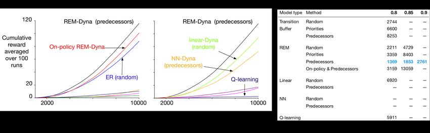
Figure 2: (a) compares variants of ER and REM-Dyna. REM-Dyna with predecessor states and Random ER accumulate significantly more
reward than all other variants, with REM-Dyna statistically significantly better (non-overlapping confidence intervals) than ER by the end of
the run. (b) shows Dyna with different models. REM-Dyna is statistically significantly better that NN-Dyna and Linear-Dyna. For NNs and
REMs, using predecessors is significantly better, unlike Linear-Dyna which learns inaccurate models. (c) Results on River Swim, with number
of steps required to obtain a ratio of 80%, 85% and 90% between the cumulative reward for the agent relative to the cumulative reward of the
optimal policy. If there is no entry, then the agent was unable to achieve that performance within the 20,000 learning steps.
deleting according to priority for both Dyna and ER. sitive. We hypothesize that this additional tuning inadvertently
Results for Continuous States. We recreate the above experi- improved the Q-learning update, rather than gaining from
ments for continuous states, and additionally explore the utility Dyna-style planning; in River Swim, Linear Dyna did poorly.
of REMs for Dyna. We compare to using a Neural Network Dyna with NNs performs poorly because the NN model is not
model—with two layers, trained with the Adam optimizer on a data-efficient; after several 1000s of more learning steps, how-
sliding buffer of 1000 transitions—and to a Linear model pre- ever, the model does finally become accurate. This highlights
dicting features-to-expected next features rather than states, as the necessity for data-efficient models, for Dyna to be effective.
in Linear Dyna. We improved upon the original Linear Dyna In Riverswim, no variant of ER was within 85% of optimal, in
by learning a reverse model and sweeping different step-sizes 20,000 steps, whereas all variants of REM-Dyna were, once
for the models and updates to q̂π . again particularly for REM-Dyna with Predecessors.
We conduct experiments in two tasks: a Continuous Grid-
world and River Swim. Continuous Gridworld is a continuous 6 Conclusion
variant of a domain introduced by [Peng and Williams, 1993], In this work, we developed a semi-parametric model learning
with (x, y) ∈ [0, 1]2 , a sparse reward of 1 at the goal, and a approach, called Reweighted Experience Models (REMs), for
long wall with a small opening. Agents can choose to move use with Dyna for control in continuous state settings. We
0.05 units up, down, left, right, which is executed successfully revisited a few key dimensions for maintaining the search-
with probability 0.9 and otherwise the environment executes a control queue for Dyna, to decide how to select states and
random move. Each move has noise N (0, 0.01). River Swim actions from which to sample. These included understanding
is a difficult exploration domain, introduced as a tabular do- the importance of using recent samples, prioritizing samples
main [Strehl and Littman, 2008], as a simple simulation of a (with absolute TD-error), generating predecessor states that
fish swimming up a river. We modify it to have a continuous lead into high-priority states, and generating on-policy tran-
state space [0, 1]. On each step, the agent can go right or left, sitions. We compared Dyna to the simpler alternative, Expe-
with the river pushing the agent towards the left. The right ac- rience Replay (ER), and considered similar design decisions
tion succeeds with low probability depending on the position, for its transition buffer. We highlighted several criteria for the
and the left action always succeeds. There is a small reward model to be useful in Dyna, for one-step sampled transitions,
0.005 at the leftmost state (close to 0), and a relatively large re- namely being data-efficient, robust to forgetting, enabling con-
ward 1.0 at the rightmost state (close to 1). The optimal policy ditional models and being efficient to sample. We developed a
is to constantly select right. Because exploration is difficult in new semi-parametric model, REM, that uses similarities to a
this domain, instead of -greedy, we induced a bit of extra ex- representative set of prototypes, and requires only a small set
ploration by initializing the weights to 1.0. For both domains, of coefficients to be learned. We provided a simple learning
we use a coarse tile-coding, similar to state-aggregation. rule for these coefficients, taking advantage of a conditional
REM-Dyna obtains the best performance on both domains, independence assumption and that we only require conditional
in comparison to the ER variants and other model-based ap- models. We thoroughly investigate the differences between
proaches. For search-control in the continuous state domains, Dyna and ER, in several microworlds for both tabular and con-
the results in Figures 2 parallels the conclusions from the tinuous states, showing that Dyna can provide significant gains
tabular case. For the alternative models, REMs outperform through the use of predecessors and on-policy transitions. We
both Linear models and NN models. For Linear models, the further highlight that REMs are an effective model for Dyna,
model-accuracy was quite low and the step-size selection sen- compared to using a Linear model or a Neural Network model.
4799Proceedings of the Twenty-Seventh International Joint Conference on Artificial Intelligence (IJCAI-18)
References [McCloskey and Cohen, 1989] Michael McCloskey and Neal J Co-
[Alain et al., 2016] Guillaume Alain, Yoshua Bengio, Li Yao, Jason hen. Catastrophic interference in connectionist networks: The
sequential learning problem. Psychology of learning and motiva-
Yosinski, Éric Thibodeau-Laufer, Saizheng Zhang, and Pascal
tion, 24:109–165, 1989.
Vincent. GSNs: generative stochastic networks. Information and
Inference: A Journal of the IMA, 2016. [Moore and Atkeson, 1993] Andrew W Moore and Christopher G
[Bagnell and Schneider, 2001] J A Bagnell and J G Schneider. Au- Atkeson. Prioritized sweeping: Reinforcement learning with less
tonomous helicopter control using reinforcement learning policy data and less time. Machine learning, 13(1):103–130, 1993.
search methods. In IEEE International Conference on Robotics [Ormoneit and Sen, 2002] Dirk Ormoneit and Śaunak Sen. Kernel-
and Automation, 2001. Based Reinforcement Learning. Machine Learning, 2002.
[Barreto et al., 2011] A Barreto, D Precup, and J Pineau. Reinforce- [Peng and Williams, 1993] Jing Peng and Ronald J Williams. Effi-
ment Learning using Kernel-Based Stochastic Factorization. In cient Learning and Planning Within the Dyna Framework. Adap-
Advances in Neural Information Processing Systems, 2011. tive behavior, 1993.
[Barreto et al., 2014] A Barreto, J Pineau, and D Precup. Policy [Pires and Szepesvári, 2016] Bernardo Avila Pires and Csaba
Iteration Based on Stochastic Factorization. Journal of Artificial Szepesvári. Policy Error Bounds for Model-Based Reinforcement
Intelligence Research, 2014. Learning with Factored Linear Models. In Annual Conference on
[Barreto et al., 2016] A Barreto, R Beirigo, J Pineau, and D Precup. Learning Theory, 2016.
Incremental Stochastic Factorization for Online Reinforcement [Schaul et al., 2016] Tom Schaul, John Quan, Ioannis Antonoglou,
Learning. In AAAI Conference on Artificial Intelligence, 2016. and David Silver. Prioritized Experience Replay. In International
[Deisenroth and Rasmussen, 2011] M Deisenroth and C E Ras- Conference on Learning Representations, 2016.
mussen. PILCO: A model-based and data-efficient approach to [Schlegel et al., 2017] Matthew Schlegel, Yangchen Pan, Jiecao
policy search. In International Conference on Machine Learning, Chen, and Martha White. Adapting Kernel Representations Online
2011. Using Submodular Maximization. In International Conference on
[French, 1999] R M French. Catastrophic forgetting in connectionist Machine Learning, 2017.
networks. Trends in Cognitive Sciences, 3(4):128–135, 1999. [Sohn et al., 2015] Kihyuk Sohn, Honglak Lee, and Xinchen Yan.
[Goodfellow et al., 2013] I J Goodfellow, M Mirza, D Xiao, Learning Structured Output Representation using Deep Condi-
A Courville, and Y Bengio. An empirical investigation of catas- tional Generative Models. In Advances in Neural Information
trophic forgetting in gradient-based neural networks. arXiv Processing Systems, 2015.
preprint arXiv:1312.6211, 2013. [Strehl and Littman, 2008] A. Strehl and M Littman. An analysis of
[Goodfellow et al., 2014] I J Goodfellow, J Pouget-Abadie, model-based Interval Estimation for Markov Decision Processes.
MehMdi Mirza, B Xu, D Warde-Farley, S Ozair, A C Courville, Journal of Computer and System Sciences, 2008.
and Y Bengio. Generative Adversarial Nets. In Advances in [Sutton and Barto, 1998] R.S. Sutton and A G Barto. Reinforcement
Neural Information Processing Systems, 2014.
Learning: An Introduction. MIT press, 1998.
[Grunewalder et al., 2012] Steffen Grunewalder, Guy Lever, Luca
[Sutton et al., 2008] R Sutton, C Szepesvári, A Geramifard, and
Baldassarre, Massi Pontil, and Arthur Gretton. Modelling transi-
M Bowling. Dyna-style planning with linear function approxima-
tion dynamics in MDPs with RKHS embeddings. In International
tion and prioritized sweeping. In Conference on Uncertainty in
Conference on Machine Learning, 2012.
Artificial Intelligence, 2008.
[Gu et al., 2016] Shixiang Gu, Timothy P Lillicrap, Ilya Sutskever,
[Sutton, 1991] R.S. Sutton. Integrated modeling and control based
and Sergey Levine. Continuous Deep Q-Learning with Model-
based Acceleration. In International Conference on Machine on reinforcement learning and dynamic programming. In Ad-
Learning, 2016. vances in Neural Information Processing Systems, 1991.
[Hamilton et al., 2014] W L Hamilton, M M Fard, and J Pineau. [Talvitie, 2017] Erik Talvitie. Self-Correcting Models for Model-
Efficient learning and planning with compressed predictive states. Based Reinforcement Learning. In AAAI Conference on Artificial
Journal of Machine Learning Research, 2014. Intelligence, 2017.
[Holmes et al., 2007] Michael P Holmes, Alexander G Gray, and [Van Hoof et al., 2015] H Van Hoof, J. Peters, and G Neu-
Charles L Isbell. Fast Nonparametric Conditional Density Estima- mann. Learning of Non-Parametric Control Policies with High-
tion. Uncertainty in AI, 2007. Dimensional State Features. AI and Statistics, 2015.
[Kveton and Theocharous, 2012] B Kveton and G Theocharous. [van Seijen and Sutton, 2015] H van Seijen and R.S. Sutton. A
Kernel-Based Reinforcement Learning on Representative States. deeper look at planning as learning from replay. In International
AAAI Conference on Artificial Intelligence, 2012. Conference on Machine Learning, 2015.
[Lever et al., 2016] Guy Lever, John Shawe-Taylor, Ronnie Stafford, [White, 2017] Martha White. Unifying task specification in rein-
and Csaba Szepesvári. Compressed Conditional Mean Embed- forcement learning. In International Conference on Machine
dings for Model-Based Reinforcement Learning. In AAAI Confer- Learning, 2017.
ence on Artificial Intelligence, 2016. [Yao et al., 2014] Hengshuai Yao, Csaba Szepesvári,
[Lin, 1992] Long-Ji Lin. Self-Improving Reactive Agents Based Bernardo Avila Pires, and Xinhua Zhang. Pseudo-MDPs
On Reinforcement Learning, Planning and Teaching. Machine and factored linear action models. In ADPRL, 2014.
Learning, 1992.
[Mairal et al., 2014] Julien Mairal, Piotr Koniusz, Zaid Harchaoui,
and Cordelia Schmid. Convolutional Kernel Networks. Advances
in Neural Information Processing Systems, 2014.
4800You can also read


