Improving Object-Based Land Use/Cover Classification from Medium Resolution Imagery by Markov Chain Geostatistical Post-Classification - MDPI
←
→
Page content transcription
If your browser does not render page correctly, please read the page content below
land
Article
Improving Object-Based Land Use/Cover
Classification from Medium Resolution Imagery
by Markov Chain Geostatistical Post-Classification
Wenjie Wang      ID
                      , Weidong Li   ID
                                          , Chuanrong Zhang *   ID
                                                                     and Weixing Zhang
 Department of Geography & Center for Environmental Sciences and Engineering, University of Connecticut,
 Storrs, CT 06269, USA; wenjie.wang@uconn.edu (W.W.); weidong.li@uconn.edu (W.L.);
 weixing.zhang@uconn.edu (W.Z.)
 * Correspondence: chuanrong.zhang@uconn.edu

 Received: 3 February 2018; Accepted: 5 March 2018; Published: 7 March 2018

 Abstract: Land use/land cover maps derived from remotely sensed imagery are often insufficient
 in quality for some quantitative application purposes due to a variety of reasons such as spectral
 confusion. Although object-based classification has some advantages over pixel-based classification in
 identifying relatively homogeneous land use/cover areas from medium resolution remotely sensed
 images, the classification accuracy is usually still relatively low. In this study, we aimed to test
 whether the recently proposed Markov chain random field (MCRF) post-classification method, that is,
 the spectral similarity-enhanced MCRF co-simulation (SS-coMCRF) model, can effectively improve
 object-based land use/cover classifications on different landscapes. Four study areas (Cixi, Yinchuan
 and Maanshan in China and Hartford in USA) with different landscapes and classification schemes
 were chosen for case studies. Expert-interpreted sample data (0.087% to 0.258% of total pixels) were
 obtained for each study area from the original Landsat images used in object-based pre-classification
 and other sources (e.g., Google satellite imagery). Post-classification results showed that the
 overall classification accuracies of the four cases were obviously improved over the corresponding
 pre-classification results by 14.1% for Cixi, 5% for Yinchuan, 11.8% for Maanshan and 5.6% for
 Hartford, respectively. At the meantime, SS-coMCRF also reduced the noise and minor patches
 contained in pre-classifications. This means that the Markov chain geostatistical post-classification
 method is capable of improving the accuracy and quality of object-based land use/cover classification
 from medium resolution remotely sensed imagery in various landscape situations.

 Keywords: Markov chain random field; spectral similarity; object-based classification; post-classification;
 accuracy improvement

1. Introduction
      Land use/land cover maps can provide critical information to many applications, such as
ecological and environmental management and urban planning. Researchers in different disciplines
showed that land cover/use data have important values in many scientific fields, such as hydrology,
agriculture and environment study [1,2]. Therefore, land cover/use data play an important role in the
study and analysis of global and regional scenarios today [2–4].
      Satellite remote sensing and GIS are common methods for mapping and detection of land use/cover
and its changes [2,5–8], which can provide timely and visual geospatial information [9–14]. Due to the
wide availability of satellite images, especially medium spatial resolution satellite images such as Landsat
images, using satellite images to detect the spatial and temporal variation of land use/cover has been
a subject undergoing intense study in remote sensing and GIS [12]. Many techniques have been developed
to classify land use/cover classes from satellite images, including pixel-based classification methods and

Land 2018, 7, 31; doi:10.3390/land7010031                                            www.mdpi.com/journal/land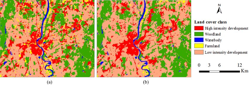
Land 2018, 7, 31                                                                                      2 of 16

object-based classification methods [5,15–17]. The advantages and disadvantages of those techniques
have been discussed in many studies [18,19]. Pixel-based classification methods have been widely used in
land use/cover classification for generating land use/cover maps from low or medium spatial resolution
remotely sensed images [11,20–22]. However, due to spectral confusion and ignoring spatial correlation,
classification results from traditional pixel-based methods are relatively low in accuracy and usually
fragmented, with the salt-and-pepper effect [23]. Although some methods (e.g., majority filter) may
remove some noise, their capabilities in classification accuracy improvement are limited because they
usually do not incorporate extra credible information from other sources to correct the misclassified pixels.
In order to overcome this effect, object-based classification methods were proposed, which allows to group
contiguous pixels with similar features into image objects for classification [24–26]. Several studies have
proved that object-based classification has better performance than pixel-based classification, especially
in fine resolution images. The results generated by object-based methods are much more homogeneous
than the results generated by pixel-based classification methods. For example, Niemeyer and Canty [27]
thought that object-oriented classification has advantages in detecting changes in finer resolution
imagery [28]. However, the results of object-based classification rely highly on the correctness of the
object generation step. On the one hand, medium resolution satellite images may not provide clear
boundaries of some ground surface objects; on the other hand, land use/cover classification at medium
or coarser spatial resolutions does not require identifying the exact shapes of ground surface individual
objects but rather aim to provide relatively large patches of generalized land use/cover classes such as
built-up area and farmland. Thus, the classification results by object-based methods using medium
resolution remotely sensed images may be relatively low in accuracy when the objects are over- or
under-segmented and identified incorrectly due to various reasons, such as spectral confusion and
over- or under-emphasis of spectral variations within/between large objects [29].
      Due to the importance of land cover/use information, the demand of accurate classification results
is on the increase. In order to improve classification accuracy, many studies have been done to develop
advanced classification methods [30–32]. However, due to the complexity of the landscape, insufficient
quality of remotely sensed data, limitations of classification methods and many other factors, classifying
remotely sensed images into a high-quality thematic map remains a challenge [32,33]. Land use/cover
maps derived from remotely sensed imagery are still insufficient in quality for many quantitative
application purposes [33–36]. Manandhar et al. [33] proved that the accuracy of land use/cover
classification can be improved by integrating related ancillary data and knowledge-based rules into
a classification. To improve the overall accuracy of a classification, the historical information about the
land use/cover was employed to estimate the a priori probability of each class [37,38]. As an additional
descriptive feature, ancillary data, such as height, slope or aspect, was also employed to improve
classification accuracy in many studies [38,39].
      In order to improve land use/cover classification accuracy, Li et al. [40] suggested a Markov
chain random field (MCRF) co-simulation approach for post-classifying the pre-classified image data
by traditional methods. This method utilizes expert-interpreted sample data from multiple sources
as high-quality sample data in MCRF co-simulation, which takes the pre-classified image data set
by a conventional classifier as an auxiliary data set. On the one hand, human eye is no doubt the
most convenient, comprehensive and reliable tool for identifying land use/cover classes; on the other
hand, more and more data sources about ground surface landscapes, such as Google satellite images,
become available. Thus, through expert-interpreted sample data and co-simulation, the method
brings extra reliable class label information and spatial correlation information into a pre-classified
image so that the classification quality can be improved. Zhang et al. [41] demonstrated that the
MCRF co-simulation (coMCRF) model can effectively improve the accuracies of land use/cover
pre-classifications generated by several different pixel-based conventional classifiers for a relative
large area with a complex landscape. To reduce the smoothing effect of spatial statistical models
(mainly caused by the circular neighborhood) in post-classification, Zhang et al. [42] modified the
coMCRF model by incorporating spectral similarity measures into a spectral similarity-enhanced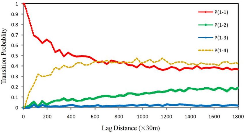
Land 2018, 7, 31 3 of 16
Land 2018, 7, x FOR PEER REVIEW 3 of 16
MCRF co-simulation (SS-coMCRF) model for land use/cover post-classification. The advantage of the
SS-coMCRF
model bymodel over the
incorporating coMCRF
spectral modelmeasures
similarity is that it into
can abetter
spectralcapture the shape features
similarity-enhanced MCRFofco-some
landsimulation
use/cover(SS-coMCRF)
objects that have
modelrelatively
for land distinct
use/coverspectral values (e.g., The
post-classification. waterbodies).
advantage of the SS-
Object-based
coMCRF model classification
over the coMCRF represents
model isanother commonly-used
that it can better capture theclassification
shape featuresapproach in land
of some land
use/cover
use/cover objects that have
classification fromrelatively
remotelydistinct
sensedspectral
imagery.values
How (e.g., waterbodies).
to improve the classification accuracy
Object-based
over object-based classification has
classifications represents another
been thus an commonly-used
important research classification approach in
topic. Although landmay
there
use/cover classification from remotely sensed imagery. How to improve the classification
be a variety of methods for improving the accuracy of object-based classifications, the SS-coMCRF accuracy
modelover object-based
can be a unique classifications
way because hasit been thus an
improves important research
classification accuracy topic. Although thereextra
by incorporating may be a
reliable
variety of methods for improving the accuracy of object-based classifications, the SS-coMCRF model
information (i.e., expert-interpreted sample data from multiple sources and land use/cover class
can be a unique way because it improves classification accuracy by incorporating extra reliable
spatial correlations). The objectives of this study are to (1) test whether and how much the MCRF
information (i.e. expert-interpreted sample data from multiple sources and land use/cover class
post-classification method (using the SS-coMCRF model) can improve the accuracies of land use/cover
spatial correlations). The objectives of this study are to (1) test whether and how much the MCRF
classifications produced by an (using
post-classification method object-based classifier from
the SS-coMCRF model)medium resolution
can improve thesatellite images;
accuracies and (2)
of land
test use/cover
the post-classification
classifications produced by an object-based classifier from medium resolution satellite by
effect on different landscapes with different classification schemes
choosing four
images; anddifferent case
(2) test the study areas. effect on different landscapes with different classification
post-classification
schemes by choosing four different case study areas.
2. Materials
2. Materials
2.1. Remote Sensing Data
2.1. Remote Sensing Data
Four cases were chosen to be used in this research: (1) a part of Cixi city, Zhejiang, China,
with upper Four cases
left werecoordinates
corner chosen to be(121 ◦ 13
used in0 47 00 E,
this 30◦ 160 42
research: 00 a
(1) part
N), of Cixi city,
recorded on 20Zhejiang,
May 2011;China,
(2) awith
part of
upper city
Yinchuan left (including
corner coordinates
some area (121°13′47′′
of nearby E,Shizuishan
30°16′42″ N), recorded
city), Ningxia, on 20
China,May with
2011;upper
(2) a part of
left corner
Yinchuan(106
coordinates city◦ (including some
100 3300 E, 38 ◦ 440area of nearby
5700 N), recorded Shizuishan
on 18 June city),2011;
Ningxia,
(3) aChina,
part ofwith upper leftcity,
Maanshan corner
Anhui,
coordinates
China, with upper (106°10′33′′ E, 38°44′57″
left corner N), recorded
coordinates (118◦ 21on 1800 June
0 27 E, 312011; (3)00 aN),
◦ 460 46 partrecorded
of Maanshan
on 19city, Anhui,2010;
August
China, with upper left corner coordinates (118°21′27″ E, 31°46′46″ N),◦ recorded 0 00 on◦ 190 August
00 2010;
(4) a part of Hartford, CT, USA, with upper left corner coordinates (72 48 4 W, 41 53 22 N), recorded
(4) a part of Hartford, CT, USA, with upper left corner coordinates (72°48′4′′ W, 41°53′22″ N), recorded
on 21 June 2011. Landsat 5 TM imagery was used in this study (see Figure 1). The images consist of
on 21 June 2011. Landsat 5 TM imagery was used in this study (see Figure 1). The images consist of
seven spectral bands, with a medium spatial resolution of 30 m for Bands 1 to 5 and 7 and a spatial
seven spectral bands, with a medium spatial resolution of 30 m for Bands 1 to 5 and 7 and a spatial
resolution of 120
resolution of 120mm forfor
Band
Band 6.6.Therefore,
Therefore, Bands
Bands 11 to to 55 and
and77were wereextracted
extracted forfor
thethe classification
classification
purpose. TheThe
purpose. images
images were
werecorrected
correctedfor
foratmospheric
atmospheric and and geometric
geometricdistortion
distortion prior
prior to use.
to use.
Figure 1. Landsat 5 images used in case studies: (a) a part of Cixi city, Zhejiang, China; (b) a part of
Figure 1. Landsat 5 images used in case studies: (a) a part of Cixi city, Zhejiang, China; (b) a part of
Yinchuan city, Ningxia, China; (c) a part of Maanshan city, Anhui, China; (d) a part of Hartford, CT,
Yinchuan city, Ningxia, China; (c) a part of Maanshan city, Anhui, China; (d) a part of Hartford, CT, USA.
USA.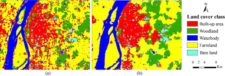
Land 2018, 7, 31                                                                                                                  4 of 16

     The image for the Cixi study area contains 722 columns by 702 rows of pixels and covers
a variety of landscape elements, including urban areas, agricultural lands, lakes, rivers and mountains.
Therefore, four major land use/cover classes were mapped, namely, built-up area, farmland, woodland
and waterbody. The image for the Yinchuan study area, which includes a part of the adjacent
Shizuishan city, contains 1354 columns by 1206 rows of pixels, with a complex landscape, including
urban areas, agricultural lands, lakes, rivers, mountains and a large area of bare lands. Therefore,
four major land use/cover classes were classified, namely, built-up area, farmland, bare land and
waterbody. Bare land refers to the areas of bare soils or rocks with little vegetation cover. Generally,
vegetation accounts for less than 15% of total cover. The image of the Maanshan study area contains
1047 columns by 800 rows of pixels. It has a more complex landscape, including urban areas,
agricultural lands, rivers, mountains and residues of iron mines. So, five major land use/cover
classes were mapped, namely, built-up area, farmland, woodland, bare land and waterbody. The image
of the Hartford study area contains 995 columns by 809 rows of pixels. The landscape covers urban
areas, agricultural lands, rivers, lakes and hills. Five major land use/cover classes were considered in
classification, namely, high intensity development, low intensity development, farmland, woodland
and waterbody. High intensity development refers to the areas with mainly constructed materials,
such as urban cores. Low intensity development means the areas with a mixture of constructed
materials and vegetation.

2.2. Expert-Interpreted Data
     In this study, the SS-coMCRF model [42] was used to improve the accuracy of land use/cover
classification by taking a pre-classified image as auxiliary data. To achieve this goal, pre-classification
map data and expert-interpreted sample data were needed. For the purposes of land use/cover class
identification and accuracy assessment, besides the Landsat images, some other reference data sources
were needed for expert-interpretation of sample data (including sample data for validation). The other
data sources we used in this study include Google earth imagery, fine resolution images from Terra
server and satellite images from DigitalGlobe. The locations of sample data were randomly selected
using ArcGIS. During the expert-interpretation process, unidentifiable pixels at selected locations
were discarded and only identifiable pixels were interpreted as sample data. For each case study area,
specific quantities of expert-interpreted sample data for post-classification and validation for each land
use/cover class are given in Table 1. The total numbers of sample data (pixel class labels) used for
post-classification for the four selected study areas are 1309 (0.258% of the total image pixels in the
study area) for Cixi, 1428 (0.087% of the total image pixels in the study area) for Yinchuan, 1401 (0.167%
of the total image pixels in the study area) for Maanshan and 1500 (0.186% of the total image pixels in
the study area) for Hartford, respectively. As an example, Figure 2 shows the spatial distributions of
the expert-interpreted sample data for post-classification and the expert-interpreted sample data for
validation for the Yinchuan study area.
      Table 1. Quantities of expert-interpreted sample datasets and validation data sets for the four case studies.

                        Expert-Interpreted     Validation                                   Expert-Interpreted     Validation
        Cixi City                                                   Yinchuan City
                       Sample Data (Pixels)   Data (Pixels)                                Sample Data (Pixels)   Data (Pixels)
       Built-up area          512                 147               Built-up area                 338                 121
        Woodland               150                 71                Farmland                     882                 324
        Waterbody              31                  14                Waterbody                     59                  20
        Farmland               616                193                Bare land                     149                 53
           Total              1309                425                   Total                     1428                518
        Maanshan        Expert-Interpreted     Validation                                   Expert-Interpreted     Validation
                                                                    Hartford City
          City         Sample Data (Pixels)   Data (Pixels)                                Sample Data (Pixels)   Data (Pixels)
       Built-up area           347                134         High intensity development           299                 94
        Woodland               208                 80                Farmland                      429                167
        Waterbody              80                 67                 Waterbody                      36                 14
        Farmland               699                269                Bare land                     114                 30
        Bare land              67                  26         Low intensity development            622                277
           Total              1401                576                   Total                     1500                582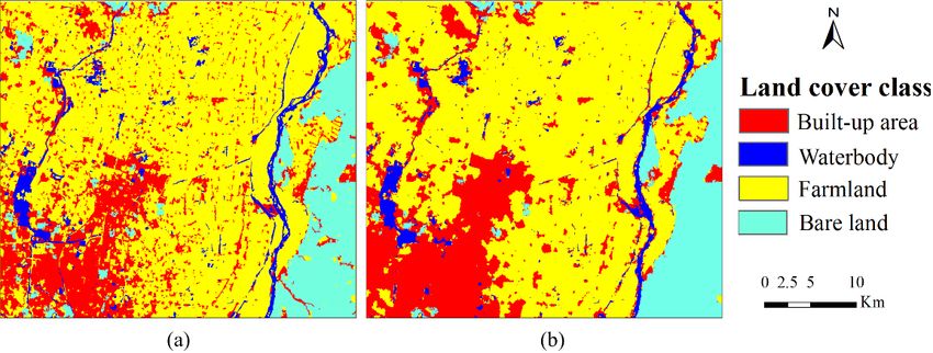
Land 2018, 7, 31 5 of 16
Land 2018, 7, x FOR PEER REVIEW 5 of 16
Land 2018, 7, x FOR PEER REVIEW 5 of 16
Figure 2. Expert-interpreted land use/cover sample data for the study area in Yinchuan: (a) a subset
Figure 2. Expert-interpreted
Expert-interpreted land
land use/cover
use/cover sample
sample data
data for the study area
area in Yinchuan: (a)
(a) aa subset
subset
Figure
of 1428 2.
sample data for MCRF co-simulation (0.087% of thefor theimage
total study pixels);
in Yinchuan:
and (b) a subset of 518
of 1428
of 1428 sample
sample data for
forMCRF
MCRFco-simulation
co-simulation(0.087% ofof
thethe
total image pixels); andand
(b) (b)
a subset of 518
sample data for data
validation. (0.087% total image pixels); a subset of
sample
518 datadata
sample for validation.
for validation.
3. Methodology
3. Methodology
3. Methodology
3.1. General Procedure
3.1. General
3.1. General Procedure
Procedure
The flow chart of the MCRF post-classification methodology using the SS-coMCRF model was
The flow
The flow chart
chart of
of the MCRF
MCRF post-classification methodology using using the
the SS-coMCRF
SS-coMCRF modelmodel was
was
shown in Figure 3. Antheobject-based post-classification
classification method methodology
was employed to generate pre-classified
shown inFigure
shown Figure3.3.An Anobject-based
object-based classification methodwas was employed to generate pre-classified
image in data. Sample classification
data for post-classification method
simulation employed to generate
and accuracy pre-classified
assessment image
were expert-
image
data. data.
Sample Sample data
datamultiple for post-classification
for post-classification simulation simulation
andimage and
accuracy accuracy assessment
assessment were were expert-
expert-interpreted
interpreted from sources, such as the original for classification, Google earth imagery,
interpreted
from from multiple sources, such asimage
the original image for classification, Google earth imagery,
fine resolution images from Terra server and satellite images from DigitalGlobe. Thesefine
multiple sources, such as the original for classification, Google earth imagery, resolution
sample data
fine resolution
images from images from
Terra Terra server and satellite images fromThese DigitalGlobe.data
These sample
split data
were split into two server and
sets, one setsatellite images
for parameter from DigitalGlobe.
estimation (i.e., estimation sample
of transiogramweremodels into
and
were
two split
sets, into
one two
set sets,
for one set
parameter for parameter
estimation estimation
(i.e., estimation(i.e.,
ofestimation of
transiogram transiogram
models and models and
cross-field
cross-field transition probability matrix) and conditioning post-classification simulation and the
cross-field transitionmatrix)
transition probability matrix) and conditioning post-classification simulation and the
other set probability
for accuracy assessment and conditioning post-classification
(i.e., validation). The estimatedsimulation and the other
parameters, set forwith
together accuracy
pre-
other set
assessment for accuracy
(i.e., assessment
validation). The (i.e.,
estimated validation).
parameters, The estimated
together with parameters,
pre-classified together
image datawith
and pre-
the
classified image data and the original remotely sensed image data, were inputs to the SS-coMCRF
classified
original image
remotely data
sensed and the
image original
data, wereremotely
inputs sensed
to the image
SS-coMCRF data, were
model inputs
for to the SS-coMCRF
post-classification.
model for post-classification.
model for post-classification.
Figure 3. The flow chart of the MCRF post-classification methodology using the SS-coMCRF model.
Figure 3. The flow chart of the MCRF post-classification methodology using the SS-coMCRF
SS-coMCRF model.
model.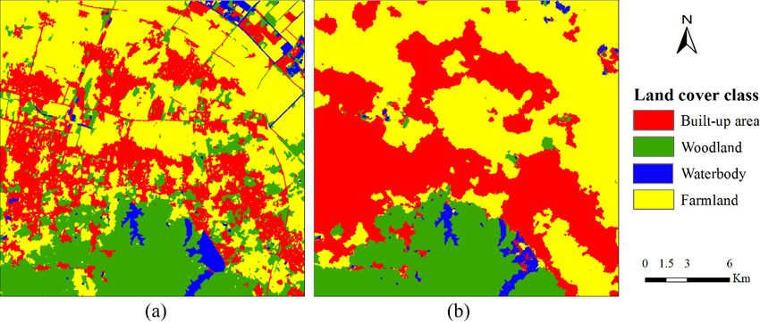
Land 2018, 7, 31                                                                                           6 of 16

3.2. Spectral Similarity-Enhanced MCRF Co-Simulation Model
     The core of the MCRF post-classification method is the coMCRF model [40] and the SS-coMCRF
model [42], which incorporate all related data into a final classification through the post-classification
operation to improve the accuracy of land use/cover classification. The coMCRF model is an extension
of the MCRF model proposed by Li [43] in order to incorporate auxiliary data. The SS-coMCRF
model is a modification of the coMCRF model in order to reduce the smoothing (or filtering) effect
in post-classification, by incorporating spectral similarity measures based on the spectral values of
the original remotely sensed image used in pre-classification. So, when the original remotely sensed
image for land use/cover classification is available, the SS-coMCRF model can be used to reduce the
loss of geometric features of some land use/cover classes in land use/cover post-classification.
     Li [43] introduced the MCRF theory and the Markov chain geostatistical approach for simulating
categorical fields. The MCRF model was derived by applying Bayes’ theorem [44] and sequential
Bayesian updating to nearest data within a neighborhood and could be visualized as a probabilistic
directed acyclic graph [40], thus being consistent with Bayesian Networks [44,45]. The conditional
independence assumption for nearest data within a neighborhood, extended from a property of Pickard
random fields, was used to simplify the MCRF full solution to a form that contains only transition
probabilities [43,46]. The transiogram concept is one of the important components in this model.
Li [47] introduced the transiogram as an accompanying spatial correlation measure of Markov chain
geostatistics. The transiogram theoretically refers to a transition probability-lag function:

                                       pij (h) = Pr( Z (u + h) = j| Z (u) = i )                               (1)

where pij represents the transition probability from class i to class j, Z(u) stands for a spatially stationary
random variable at a specific location u and h, as a vector variable, refers to the separate distance
between the two spatial points u and u + h. Visually, the transiogram is a transition probability-lag
curve. While an auto-transiogram pii (h) represents the autocorrelation of a land use/cover class,
a cross-transiogram pij (h) (i 6= j) represents the cross-correlation of a pair of land use/cover classes.
As transition probability, cross-transiograms are asymmetric and can be unidirectional.
     Considering four nearest data and the quandrantal neighborhood (i.e., seeking one nearest
datum from each quadrant sectoring the circular search area if there are nearest data in the quadrant),
the SS-coMCRF model [42] can be given as:

                                    p[i0 (u0 )|i1 (u1 ), . . . , i4 (u4 ); r0 (u0 ); Spectrum]
                                         qi0 r0 pi1 i0 (h10 )Si1 i0 ∏4g=2 pi0 i g (h0g )Si0 i g               (2)
                             =       n
                                    ∑ f =1 [q f0 r0 pi1 f0 (h10 )Si1 f0 ∏4g=2 p f0 i g (h0g )S f0 i g ]
                                       0

where u represents the location vector of a pixel, i0 refers to the land use/cover class of the unobserved
pixel at location u0 ; i1 to i4 are the states of the four nearest neighbours around the unobserved location
u0 within a quadrantal neighbourhood; the left hand side of the equation is the posterior probability
of class i0 ; pi0 i g (h0g ) is a specific transition probability over the separation distance h0g between
locations u0 and ug , which can be fetched from a corresponding transiogram model; qi0 r0 represents
the cross-field transition probability from class i0 at the location u0 in the primary field being simulated
to class r0 at the co-location in the covariate field (here the pre-classified image); and Spectrum here
means the spectral data of the original remotely sensed image for pre-classification, which are used to
calculate the spectral similarity-based constraining factor Si0 i g .
     In above equation, the spectral similarity-based constraining factor S is calculated as:
                                              (
                                                  1.0,                                          il 6= ik
                                 Si l i k =                                                                   (3)
                                                  ρil ik (xl , yk ) × Jil ik (xl , yk ),        il = ik
Land 2018, 7, 31 7 of 16
where il 7,isx FOR
Land 2018, the PEER use/cover class of pixel l; ρil ik and Jil ik are the spatial correlation measure
land REVIEW 7 of 16
(i.e., correlation coefficient) and Jaccard index of the spectral vectors (i.e., spectral values of different
bands) xl and
bands) andy of pixel
of pixel l and
l and pixelpixel k, respectively.
k, respectively. Seefor[42]
See [42] for a detailed
a detailed description
description of the SS-
of the SS-coMCRF
k
coMCRF
model and model and thesimilarity-based
the spectral spectral similarity-based constraining
constraining factor. factor.
3.3. Inputs and Outputs for the SS-coMCRF Model
In order toto perform
perform simulation
simulation using the the SS-coMCRF
SS-coMCRF model, cross-field transition probability
matrix and
and transiogram
transiogrammodelsmodelsare required
are required as input
as inputparameters,
parameters,besides pre-classified
besides imageimage
pre-classified data,
original
data, remotely
original sensedsensed
remotely image image
and expert-interpreted
and expert-interpreted samplesample
data. Transiogram models provide
data. Transiogram models
transition
provide probability
transition values values
probability at anyatneeded
any needed lag values. Li and
lag values. Li andZhang
Zhang [48]
[48]proved
provedthat
that linear
interpolation is more efficient than model fitting when when samples
samples are adequate
adequate and and experimental
experimental
transiograms are arereliable.
reliable.ToTotake the the
take advantage
advantageof theoflinear interpolation
the linear method,
interpolation sufficient
method, expert-
sufficient
interpreted samplesample
expert-interpreted data were selected
data were to create
selected reliable
to create experimental
reliable experimental transiograms
transiogramsininthis
thisstudy.
study.
Figure 4 shows a subset of transiogram models estimated from the expert-interpreted sample dataset
the Cixi
for the Cixicase
casestudy.
study.Table
Table2 2shows
shows the the cross-field
cross-field transition
transition probability
probability matrix,
matrix, which
which expresses
expresses the
the cross
cross correlations
correlations between
between classes
classes of sample
of sample datadata
and and the pre-classified
the pre-classified imageimage
data.data.
One One cross-
cross-field
field transition
transition probability
probability matrix ismatrix
enough is for
enough for a co-simulation
a collocated collocated co-simulation
conditioned onconditioned on data
one auxiliary one
auxiliary
set databeset
and it can and it can
calculated be calculated
using the transitions using thethe
from transitions from the
selected sample selected
points sample
to their points to
corresponding
their corresponding
collocated collocated
points in the pointsimage
pre-classified in the [40].
pre-classified image [40].
Table 2.2. Cross-field transition probability matrix from classes of the
Table the expert-interpreted
expert-interpreted dataset to
classes of the pre-classified
pre-classified data
data by
by the
the object-based
object-based classification
classification for
for the
theCixi
Cixicase
casestudy.
study.
Cross-Field
Cross-Field Transition
Transition Probability
Probability
Pre-Classification Data
Pre-Classification Data
Class ** C1 C2 C3 C4
Class ** C1 C2 C3 C4
C1 0.602 0.077 0.005 0.317
C1 C2 0.602 00.077 0.932
0.005 0.317
0 0.068
Expert-interpreted sample data C2 0 0.932 0 0.068
Expert-interpreted sample data C3 0.231 0.231 0.538 0
C3 0.231 0.231 0.538 0
C4 C4 0.086 0.086 0.126 0.126
0.007 0.007
0.781 0.781
** C1—Built-up area;
** C1—Built-up area;C2—Woodland; C3—Waterbody;
C2—Woodland; C3—Waterbody; C4—Farmland.
C4—Farmland.
Figure 4.
Figure 4. AAsubset
subsetofoftransiogram
transiogrammodels
models estimated
estimated from thethe
from expert-interpreted
expert-interpretedsample datadata
sample for the
for
Cixi case study. P(1-1) denotes the auto transition probability of built-up area. P(1-2)
the Cixi case study. P(1-1) denotes the auto transition probability of built-up area. P(1-2) denotes denotes the
cross-transition
the cross-transitionprobability from
probability from built-up
built-uparea
areatotowoodland.
woodland.P(1-3)
P(1-3) denotes
denotes the cross-transition
the cross-transition
probability from
probability from built-up
built-up area
area to
to waterbody.
waterbody. P(1-4)
P(1-4) denotes
denotes the
the cross-transition
cross-transition probability
probability from
from
built-up area
built-up area to
to farmland.
farmland. Lag
Lag is
is the
the separate
separate distance
distance between
between aa pair
pair of
of data
data points.
points.
For each simulation case, the SS-coMCRF model generated one hundred of simulated
realizations. Occurrence probabilities of land use classes at all pixels were estimated from the
simulated realization maps. Based on the maximum probabilities, an optimal post-classification map
was achieved for each case. After that, confusion matrix and Kappa coefficient were used to calculateLand 2018, 7, 31 8 of 16
For each simulation case, the SS-coMCRF model generated one hundred of simulated realizations.
Occurrence probabilities of land use classes at all pixels were estimated from the simulated realization
maps. Based on the maximum probabilities, an optimal post-classification map was achieved for each
case. After that, confusion matrix and Kappa coefficient were used to calculate the accuracy of each
optimal post-classification map and pre-classified image using the corresponding validation data set.
3.4. Object-Based Classification
The object-based classification (OBC) approach was initially introduced in 1970s [49,50]. With the
increased demand for OBC methods, many GIS software systems are available to use this kind
of methods for classification. ENVI is one of the most commonly used software systems and it
provides a K-Nearest Neighbor (KNN) object-based classification method. Due to its simplicity in
implementation, clarity in theory and good performance in classification, KNN has become one of
the most commonly used OBC methods. Therefore, the KNN method was employed for object-based
classification in this study. The KNN object-based classification process has two steps: segmentation
and classification. Segmentation is the way to partition a remote sensing image into different objects by
merging pixels with similar attributes [51,52]. Segmentation is the most important part in object-based
classification, because it can divide an image into homogeneous objects and ensure the classification
results more accurate [50].
The KNN method was employed to segment an original remotely sensed image into land use
segments and then chose a set of segments as training data based on different land use/cover classes
to classify the segments. The parameters of segmentation were chosen based on visual inspection and
researcher’s experience. Too many segments could increase processing time and were not necessary.
In segment settings, the value of parameter Edge was set to 30 for detecting edges of features where
objects of interest have sharp edges. Adjacent segments with similar spectral attributes can be merged.
In this study, the value of Merge Level was set to 90 to merge over-segmented areas by using the Full
Lambda Schedule algorithm. The value of Texture Kernel Size is the size (in pixels) of a moving box
centered over each pixel in the image for computing texture attributes, which was set to 3. The resulting
segments can clearly show boundaries of each land cover type. Because we conducted example-based
classification, training data for classification were selected from segmented components. The number
of object-based training samples was determined based on the researcher’s experience and 1000 object
samples were randomly selected for each study case. Each training sample was chosen to contain
only one land cover type. Based on the training samples and segments’ proximity to neighboring
training regions, the KNN method assigned segments into different classes with the highest class
confidence value.
4. Results and Discussions
4.1. Case 1
Figure 5 shows the pre-classification map and the corresponding MCRF post-classification map
for the Cixi study area. Table 3 provides a comparison of classification accuracies between the
pre-classification and the MCRF post-classification. The overall accuracy (OA) of the pre-classification
map is 70.6%. However, the OA for the MCRF post-classification map is 84.7%. The overall
improvement in land use/cover classification accuracy is 14.1%. The MCRF post-classification
increased kappa coefficient from 0.552 to 0.762. In the pre-classification map, some built-up area
pixels were misclassified into woodland and farmland. Due to the complexity of the landscape in this
area, it is difficult to distinguish built-up area from woodland and farmland by purely using the KNN
OBC method. After post-processing by MCRF co-simulation using the SS-coMCRF model, there are
obvious increases in the producer’s accuracies of built-up area (increase from 65% to 87%), woodland
(increase from 82% to 89%) and farmland (increase from 71% to 84%). In terms of the user’s accuracies,
MCRF post-classification made improvements in the classification of built-up area (increase from 79%Land 2018, 7, 31 9 of 16
to 84%) and woodland (increase from 56% to 85%). However, the producer’s accuracy of waterbody
decreased (from 57% to 50%). Considering that waterbody is a minor class, its accuracy assessment
is not reliable and has little impact on the overall accuracy. Apparently, MCRF post-classification
corrected many misclassified pixels and also reduced small noise features. A drawback is that some
Land 2018, 7, x FOR PEER REVIEW 9 of 16
linear features (mainly roads or water channels here, pre-classified as linear objects of built-up area,
woodland
objects of or waterbody),
built-up which wereorpartially
area, woodland captured
waterbody), by the
which werepre-classification,
partially capturedwere
bylost
theinpre-
the
MCRF post-classification map (Figure 5).
classification, were lost in the MCRF post-classification map (Figure 5).
Figure 5.
Figure 5. Land
Landuse/cover
use/coverclassification results
classification forfor
results thethe
Cixi study
Cixi area:
study (a) pre-classification
area: map;
(a) pre-classification (b)
map;
MCRF post-classification map.
(b) MCRF post-classification map.
Table 3. Accuracy assessment for pre-classification and corresponding post-classification for the Cixi
Table 3. Accuracy assessment for pre-classification and corresponding post-classification for the Cixi
study area.
study area.
Object-Based Pre-Classification MCRF Post-Classification
Object-Based Pre-Classification User’s MCRF Post-Classification User’s
Class ** C1 C2 C3 C4 Total C1 C2 C3 C4 Total
Accuracy (%) Accuracy (%)
User’s User’s
Class
C1 ** C196 C2 2 C31 C422 Total
121 79 C1128 C2 2 C31 C422 Total153 84
Accuracy (%) Accuracy (%)
C2 12 58 2 31 109 56 2 63 0 9 80 85
C1
C3 960 2 0 18 222 12110 79 80 128 0 2 0 17 220 1537 84100
C2
C4 1239 5811 23 31138 109185 56 72 2 17 63 6 06 9162 80185 8585
C3
Total 0147 0 71 814 2193 10425 80 0 147 0 71 7 14 0193 7425 100
C4
Producer’s 39 11 3 138 185 72 17 6 6 162 185 85
65 82 57 71 70.6 87 89 50 84 84.7
Total(%)
accuracy 147 71 14 193 425 147 71 14 193 425
Producer’s ** C1—Built-up area; C2—Woodland; C3—Waterbody; C4—Farmland.
65 82 57 71 70.6 87 89 50 84 84.7
accuracy (%)
4.2. Case 2 ** C1—Built-up area; C2—Woodland; C3—Waterbody; C4—Farmland.
Table
4.2. Case 2 4 and Figure 6 present the pre-classification results by OBC and the corresponding post-
classification results by SS-coMCRF for the Yinchuan study area. Compared with the pre-
Table 4 and
classification, Figure post-classification
the MCRF 6 present the pre-classification
improved the OA results
by 5%.by All
OBC and have
classes the corresponding
improvement
post-classification results by SS-coMCRF for the Yinchuan study area. Compared
in both producer’s accuracy and user’s accuracy. The MCRF post-classification increased kappawith the pre-classification,
the MCRF post-classification
coefficient from 0.650 to 0.746. improved the OA by 5%. All
In the pre-classification classes
map, have
bare landimprovement
and built-upinarea
bothwere
producer’s
highly
accuracy and user’s accuracy. The MCRF post-classification increased kappa coefficient
misclassified due to the confusion of their spectral values with farmland in the remotely sensed from 0.650 to
0.746. In the pre-classification map, bare land and built-up area were highly
image, thus resulting in low producer’s accuracy for built-up area (69%) and bare land (68%). misclassified due to the
confusion
Meanwhile, oflow
their spectral
user’s values(65%)
accuracy withalso
farmland in the
occurred for remotely sensed
the built-up area image, thus resulting inmap
in the pre-classification low
producer’s accuracy for built-up area (69%) and bare land (68%). Meanwhile, low
due to the misclassification of some built-up area pixels into bare land and farmland. The MCRF post- user’s accuracy
(65%) also occurred
classification operation forchanged
the built-up area in the
this situation by pre-classification map due to the misclassification
correcting some misclassifications. Both producer’s
of some built-up
accuracies areaaccuracies
and user’s pixels intoofbare
the land and farmland.
four land The MCRF
use/cover classes werepost-classification
increased after MCRF operation
post-
changed this situation by correcting some misclassifications. Both
classification. Similarly, most noise was removed in the post-classification map. producer’s accuracies and user’s
accuracies of the four land use/cover classes were increased after MCRF post-classification. Similarly,
mostTable
noise 4.was removed
Accuracy in the post-classification
assessment map.
for pre-classification and corresponding post-classification for the
Yinchuan study area.
Object-Based Classification MCRF Post-Classification
User’s User’s
Class ** C1 C2 C3 C4 Total C1 C2 C3 C4 Total
Accuracy (%) Accuracy (%)
C1 83 33 0 11 128 65 97 26 0 9 132 73
C2 32 287 5 6 330 87 21 294 3 5 323 91
C3 0 2 15 0 17 88 0 2 17 0 19 89
C4 6 2 0 36 44 82 3 2 0 39 44 89
Total 121 324 20 53 518 121 324 20 53 518Land 2018, 7, 31 10 of 16
Table 4. Accuracy assessment for pre-classification and corresponding post-classification for the
Yinchuan study area.
Object-Based Classification MCRF Post-Classification
User’s User’s
Class ** C1 C2 C3 C4 Total C1 C2 C3 C4 Total
Accuracy (%) Accuracy (%)
C1 83 33 0 11 128 65 97 26 0 9 132 73
C2 32 287 5 6 330 87 21 294 3 5 323 91
C3 0 2 15 0 17 88 0 2 17 0 19 89
C4 6 2 0 36 44 82 3 2 0 39 44 89
Total 121 324 20 53 518 121 324 20 53 518
Producer’s
69 89 75 68 81.3 80 91 85 74 86.3
accuracy (%)
** C1—Built-up area; C2—Farmland; C3—Waterbody; C4—Bare land.
Land 2018, 7, x FOR PEER REVIEW 10 of 16
Figure 6.
Figure 6. Land
Land use/cover
use/coverclassification
classificationresults
resultsfor
forthe
theYinchuan
Yinchuan study
study area:
area: (a)
(a) pre-classification
pre-classification map;
map;
(b) MCRF post-classification.
(b) MCRF post-classification.
4.3. Case 3
4.3. Case 3
Results for Case 3 are provided in Figure 7 and Table 5. There are some residues of iron mines
Results for Case 3 are provided in Figure 7 and Table 5. There are some residues of iron mines
existing in the Maanshan city, which were classified as bare land. It is difficult to distinguish this kind
existing in the Maanshan city, which were classified as bare land. It is difficult to distinguish this kind
of bare land from built-up area in this study area. That is why the pre-classification map has a
of bare land from built-up area in this study area. That is why the pre-classification map has a relatively
relatively low producer’s accuracy for bare land (58%). Before post-classification, some bare land
low producer’s accuracy for bare land (58%). Before post-classification, some bare land pixels were
pixels were misclassified as built up area. After post-processing by the SS-coMCRF model, some
misclassified as built up area. After post-processing by the SS-coMCRF model, some misclassified
misclassified bare land pixels were corrected. In the pre-classification map, because of spectral
bare land pixels were corrected. In the pre-classification map, because of spectral overlap of farmland
overlap of farmland with built-up area and woodland in the remotely sensed image, some pixels of
with built-up area and woodland in the remotely sensed image, some pixels of built-up area and
built-up area and woodland were misclassified as farmland and similarly some pixels of farmland
woodland were misclassified as farmland and similarly some pixels of farmland were misclassified
were misclassified as built-up area and woodland, thus resulting in relatively low producer’s
as built-up area and woodland, thus resulting in relatively low producer’s accuracies (e.g., 63% for
accuracies (e.g., 63% for woodland and 70% for farmland). Because some waterbody areas were
woodland and 70% for farmland). Because some waterbody areas were covered by water plants or
covered by water plants or other vegetation and those pixels were misclassified as farmland or
other vegetation and those pixels were misclassified as farmland or woodland, the producer’s accuracy
woodland, the producer’s accuracy of waterbody was 85%. The MCRF post-classification operation
of waterbody was 85%. The MCRF post-classification operation changed this situation by correcting
changed this situation by correcting many misclassifications and consequently increased the OA and
many misclassifications and consequently increased the OA and kappa coefficient by 11.8% and 0.165
kappa coefficient by 11.8% and 0.165 (from 0.591 to 0.756), respectively. Specifically, post-
(from 0.591 to 0.756), respectively. Specifically, post-classification improved the producer’s accuracies
classification improved the producer’s accuracies of built-up area, woodland, farmland and bare land
of built-up area, woodland, farmland and bare land by 9%, 13%, 13% and 19%, respectively and
by 9%, 13%, 13% and 19%, respectively and improved their user’s accuracies by 19%, 13%, 8% and
improved their user’s accuracies by 19%, 13%, 8% and 9%, respectively. The filtering effect of the
9%, respectively. The filtering effect of the MCRF post-classification method to noise was also clear.
MCRF post-classification method to noise was also clear.woodland, the producer’s accuracy of waterbody was 85%. The MCRF post-classification operation
changed this situation by correcting many misclassifications and consequently increased the OA and
kappa coefficient by 11.8% and 0.165 (from 0.591 to 0.756), respectively. Specifically, post-
classification improved the producer’s accuracies of built-up area, woodland, farmland and bare land
by 9%,
Land 2018,13%,
7, 31 13% and 19%, respectively and improved their user’s accuracies by 19%, 13%, 8% and
11 of 16
9%, respectively. The filtering effect of the MCRF post-classification method to noise was also clear.
Figure 7.
Figure 7. Land
Land use/cover
use/coverclassification
classification results
results for
for the
the Maanshan
Maanshan study
study area:
area: (a)
(a) pre-classification
pre-classification map;
map;
(b) MCRF post-classification map.
(b) MCRF post-classification map.
Table 5. Accuracy assessment for pre-classification and corresponding SS-coMCRF post-classification
for the Maanshan study area.
Object-Based Pre-Classification MCRF Post-Classification
User’s User’s
Class ** C1 C2 C3 C4 C5 Total C1 C2 C3 C4 C5 Total
Accuracy (%) Accuracy (%)
C1 101 9 0 51 7 168 60 112 2 0 23 4 141 79
C2 4 50 5 23 0 82 61 1 61 3 16 1 82 74
C3 0 3 57 0 2 66 92 0 2 62 1 0 65 95
C4 28 18 4 187 2 235 78 19 15 1 223 1 259 86
C5 1 0 1 8 15 25 60 2 0 1 6 20 29 69
Total 134 80 67 269 26 576 134 80 67 269 26 576
Producer’s
75 63 85 70 58 71.2 84 76 92 83 77 83.0
accuracy (%)
** C1—Built-up area; C2—Woodland; C3—Waterbody; C4—Farmland; C5—Bare land.
4.4. Case 4
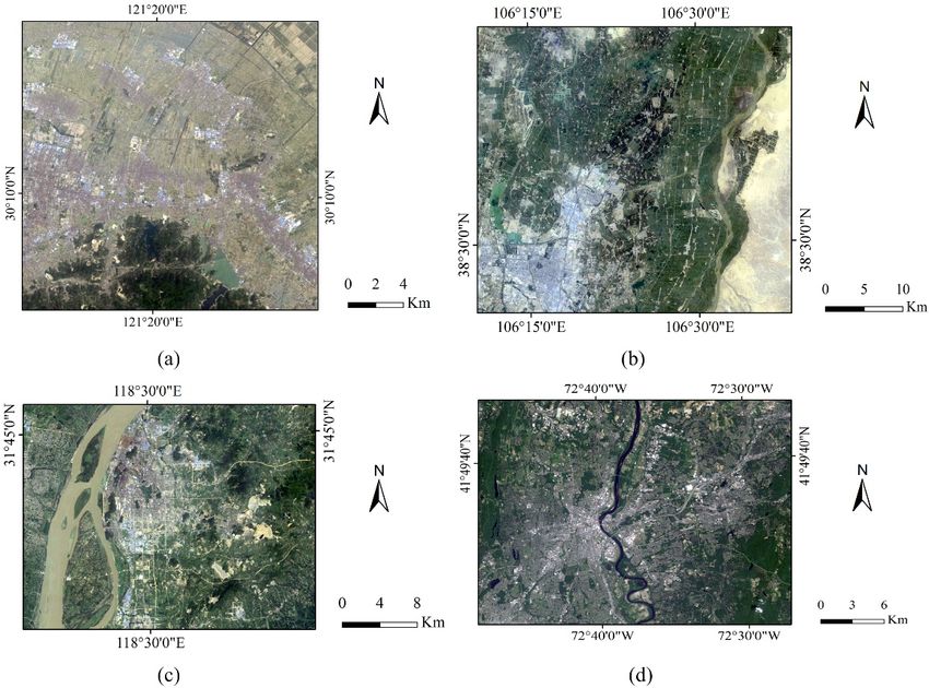
Hartford area has quite different landscape compared with other cases. The landscape was
classified into five classes, including high intensity development, low intensity development,
waterbody, farmland and woodland (Figure 8). Due to the complex landscape and the similarity
between high intensity development and low intensity development, it is hard to distinguish these
two classes. Therefore, many pixels of low intensity development were misclassified into high
intensity development in the pre-classification map (Table 6). Therefore, high intensity development
had a relatively low producer’s accuracy (69%). MCRF post-classification was able to correct some
misclassified pixels and the producer’s accuracy of high intensity development was improved to 79%.
Meanwhile, farmland was also pre-classified with very low accuracy, mainly due to its spectral overlap
with developed area (i.e., both high and low intensity development here). MCRF post-classification
improved the producer’s accuracy of farmland by 6%. The complex landscape and the local living
style (i.e., residential houses are usually scattered in forest or farmland) resulted in high spectral
confusion among land use/cover classes except for waterbody. That should be the major reason why
the pre-classification OA was relatively low (74.6%), even if waterbody was pre-classified with high
accuracy. MCRF post-classification improved the OA by 5.6%. The MCRF post-classification increased
kappa coefficient from 0.633 to 0.711.Land 2018, 7, 31 12 of 16
Table 6. Accuracy assessment for pre-classification and corresponding post-classification for the
Hartford study area.
Object-Based Pre-Classification MCRF Post-Classification
User’s User’s
Class ** C1 C2 C3 C4 C5 Total C1 C2 C3 C4 C5 Total
Accuracy (%) Accuracy (%)
C1 65 17 0 2 43 127 51 74 12 0 1 33 120 62
C2 6 140 0 3 31 180 78 5 147 0 3 27 182 81
C3 0 0 12 0 0 12 100 0 0 12 0 0 12 100
C4 11 6 0 21 7 45 46 5 4 0 22 5 36 61
C5 12 4 2 4 196 218 90 10 4 2 4 212 232 91
Total 94 167 14 30 277 582 94 167 14 30 277 582
Producer’s
69 84 86 70 71 74.6 79 88 86 73 77 80.2
accuracy (%)
** C1—High intensity development; C2—Woodland; C3—Waterbody; C4—Farmland; C5—Low intensity development.
Land 2018, 7, x FOR PEER REVIEW 12 of 16
Figure 8.
Figure 8. Land
Land use/cover
use/cover classification
classification results
results for
for the
the Hartford
Hartford study
study area:
area: (a)
(a) pre-classification map;
pre-classification map;
(b) MCRF post-classification.
(b) MCRF post-classification.
4.5. Discussions
4.5. Discussions
In this study, the KNN method was used to represent the OBC approach as the pre-classifier.
In this study, the KNN method was used to represent the OBC approach as the pre-classifier.
The MCRF post-classification method improves land use/cover classification accuracy by taking extra
The MCRF post-classification method improves land use/cover classification accuracy by taking
reliable information (expert-interpreted sample data from multiple sources and class spatial
extra reliable information (expert-interpreted sample data from multiple sources and class spatial
correlations estimated from the sample data) into a pre-classification that is previously performed by
correlations estimated from the sample data) into a pre-classification that is previously performed
a conventional pre-classifier, usually based on spectral data of an original remotely sensed image. It
by a conventional pre-classifier, usually based on spectral data of an original remotely sensed image.
does not matter which method or what kind of methods was used to perform the pre-classification.
It does not matter which method or what kind of methods was used to perform the pre-classification.
Depending on image quality, landscape complexity, classification scheme and pre-classification
Depending on image quality, landscape complexity, classification scheme and pre-classification
operation, pre-classification accuracy may be relatively high or low; consequently, corresponding
operation, pre-classification accuracy may be relatively high or low; consequently, corresponding
accuracy improvement by post-classification may be different (small or large). What we aim to
accuracy improvement by post-classification may be different (small or large). What we aim to explore
explore in this study is that whether the MCRF post-classification method (here the SS-coMCRF
in this study is that whether the MCRF post-classification method (here the SS-coMCRF model) can
model) can improve the accuracy of the classification results generated by the OBC approach, by
improve the accuracy of the classification results generated by the OBC approach, by incorporating
incorporating extra reliable information that can be easily available. Although the OBC approach is
extra reliable information that can be easily available. Although the OBC approach is segment-based
segment-based and the SS-coMCRF model is pixel-based, this does not mean that the SS-coMCRF
and the SS-coMCRF model is pixel-based, this does not mean that the SS-coMCRF model cannot be
model cannot be applied to the classification maps generated by an object-based method. The testing
applied to the classification maps generated by an object-based method. The testing cases in this
cases in this study showed that the pre-classification results generated by the KNN method is
study showed that the pre-classification results generated by the KNN method is relatively low and
relatively low and considerable accuracy improvement (5% to 14% depending on different landscape
considerable accuracy improvement (5% to 14% depending on different landscape cases) could be
cases) could be achieved and some noise (including misclassified small segments) also could be
achieved and some noise (including misclassified small segments) also could be removed by the MCRF
removed by the MCRF post-classification method.
post-classification method.
There are no strict requirements on multiple source reference images for interpreting sample
There are no strict requirements on multiple source reference images for interpreting sample
data, because what the MCRF post-classification method needs are just the land cover/use class labels
data, because what the MCRF post-classification method needs are just the land cover/use class
of some sample pixels rather than the whole images. So, reference images can include the original
labels of some sample pixels rather than the whole images. So, reference images can include the
image for pre-classification, images at the same or similar resolutions and images with finer
resolutions. Fine-resolution images are better for discerning the land cover/use classes of sample
pixels. While widely-used classifiers mainly use spectral values for classification, human eye can
utilize much more information (such as context information) to discern the land cover/use class of a
pixel in an image. So, human eye observation may discern the correct land cover/use classes of many
pixels in an image, even if some of them cannot be correctly classified in a classification. As long asLand 2018, 7, 31 13 of 16
original image for pre-classification, images at the same or similar resolutions and images with finer
resolutions. Fine-resolution images are better for discerning the land cover/use classes of sample
pixels. While widely-used classifiers mainly use spectral values for classification, human eye can
utilize much more information (such as context information) to discern the land cover/use class of
a pixel in an image. So, human eye observation may discern the correct land cover/use classes of many
pixels in an image, even if some of them cannot be correctly classified in a classification. As long as
the landscape did not change substantially (i.e., the nature of land cover/use did not change) in the
study area during the time change, reference images at similar time or even in different seasons are
suitable to use. In case some pre-selected pixels cannot be clearly discerned, they can be discarded or
alternative discernable pixels at nearby places can be used. If one source (e.g., Google satellite imagery)
is not sufficient for interpreting sample data, more data sources may be used. So, this sample data
expert-interpretation process seems ambiguous but in fact it is practical, given the availability of many
online and offline data sources at the present time.
One limitation of the MCRF post-classification method is that interpreting the needed sample
dataset from multiple sources for performing co-simulation may be somewhat time consuming.
Currently, this is the main overhead for improving land use/cover classification quality using the
MCRF approach. Although a higher density of expert-interpreted sample data may result in larger
accuracy improvement in post-classification, the accuracy improvement rate quickly decreases with
increasing density of sample data, as demonstrated by Li et al. [40] and Zhang et al. [42]. Therefore,
the basic requirement for the number of expert-interpreted sample data is that they should suit the
estimation of reliable parameters for MCRF co-simulation.
5. Conclusions
This study demonstrated that the MCRF post-classification method (i.e., the SS-coMCRF model
here) is effective in improving the accuracies of object-based land use/cover classification maps
(generated by the OBC approach using the KNN method in this study) from medium resolution
remotely sensed images with different landscapes and classification schemes. Specifically, in our
case studies, MCRF post-classification operation improved the OAs of object-based land use/cover
classifications by 14.1%, 5%, 11.8% and 5.6% for the Cixi, Yinchuan, Maanshan and Hartford study
areas, respectively. Such accuracy improvement should be attributed to the incorporation of the
expert-interpreted sample data and spatial correlation information, which can help correct a large
portion of misclassified pixels in segments in various landscape situations. Besides improving
classification accuracy, MCRF post-classification also can effectively remove classification noise or
minor sizes of patches to a large extent, thus improving recognition of land use/cover patterns.
Therefore, the MCRF post-classification method is much more than a filter that aims to remove
classification noise and minor sizes of patches, because the filtering methods do not incorporate extra
credible information from other sources into the post-classification and thus they may not improve
much or may even reduce classification accuracy (Zhang et al. 2016 [41]).
Acknowledgments: This research is partially supported by USA NSF grant No. 1414108. Authors have the sole
responsibility to all of the viewpoints presented in the paper.
Author Contributions: Wenjie Wang Weidong Li, Chuanrong Zhang and Weixing Zhang contributed to the
research design. Wenjie Wang Weidong Li and Chuanrong Zhang contributed to the writing of the paper.
Wenjie Wang undertook analysis of data. Wenjie Wang, Weidong Li, Chuanrong Zhang and Weixing Zhang
contributed to the revisions and critical reviews from the draft to the final stages of the paper.
Conflicts of Interest: The authors declare no conflict of interest.
References
1. Weng, Q. A remote sensing—GIS evaluation of urban expansion and its impact on surface temperature in
the Zhujiang Delta, China. Int. J. Remote Sens. 2001, 22, 1999–2014. [CrossRef]You can also read