Water quality and water availability at Gårdstånga Nygård - Lina Lennklev - Bachelor thesis

Bachelor thesis
TVVR 20/4001

Water quality and water
availability at Gårdstånga
Nygård

______________________________________
Lina Lennklev

Division of Water Resources Engineering
Department of Building and Environmental Technology
Lund University

Water quality and water availability at
 Gårdstånga Nygård

By:
Lina Lennklev

Bachelor Thesis

Division of Water Resources Engineering
Department of Building & Environmental Technology
Lund University
Box 118
221 00 Lund, Sweden

Bachelor Thesis
Division of Water Resources Engineering
Department of Building & Environmental Technology
Lund University

 English title: Water quality and water availability at Gårdstånga
 Nygård
 Author(s): Lina Lennklev
 Supervisor: Magnus Persson
 Examiner: Linus Zhang
 Language English
 Year: 2020
 Keywords: Water resource management; Water quality;
 Agriculture; Water balance; Constructed wetlands;
 Surface water bodies

 i

ii

iii

Acknowledgements

This bachelor’s degree project spanned over the entirety of my sixth term of
studying to become a civil engineer during the spring of 2020. The project was
carried out with the help of the Division of Water Resource Engineering.
 I would like to direct a special thanks to my supervisor Magnus Persson
at the Division of Water Resource Engineering for patiently answering my
questions and helping me forward throughout the project. I would also like to
thank Gustaf Ramel, the owner of Gårdstånga Nygård, for welcoming me to his
farm and making this project possible, and Tette Alström at Ekologigruppen for
providing me with information crucial for the completion of this project. Thanks
to Shokoufeh Salimi at the Division for Water Resource Engineering for her
support throughout the project. I would like to thank my dear friends Emma
Simonsson and Felicia Montan, my father Håkan, my brother Pontus and my
little sister Astrid for very graciously agreeing to help me execute my field
investigations. Lastly, I would like to thank my boyfriend as well as best friend
August for helping and supporting me in the fun and challenging time during
which this project was carried out.

 iv

v

Abstract

The report investigated partly how agriculture on and near Gårdstånga Nygård
affected the water quality in nearby surface water bodies during the period of
testing, and partly whether the supply of water in the Rödabäck river basin is
large enough to enable the construction of a well-functioning irrigation pond.
The water quality was evaluated by collecting water samples in the field,
reading the values of these samples for various water quality parameters and
finally an evaluation of said values. The conclusion of the study on water
quality was that it was not possible to find any reason to believe that agriculture
at and near Gårdstånga Nygård had any considerable negative effect on the
water quality of the nearby surface water bodies during the period in which the
water samples were collected.
 The conclusion that could be drawn as a result of the study on the
availability of water in the river basin was that a study in the form included in
this report is not accurate enough to say with sufficient certainty whether the
availability of water in the river basin is large enough to enable the construction
of an effective irrigation pond.

 vi

vii

Table of Contents

1. INTRODUCTION ............................................................................... 1
 1.1 Purpose ............................................................................................. 2

 2.1 Gårdstånga Nygård ................................................................................ 3
 2.1.1 Current water management system......................................................... 3
 2.1.2 Fertilization of agricultural fields during testing ............................................ 8
 2.1.3 Future constructed wetland ........................................................................... 8

 2.2 Water quality ........................................................................................... 9
 2.2.1 Agricultural leaching ................................................................................... 9
 2.2.2 Dissolved solids and electrical conductivity .......................................... 10
 2.2.3 Phosphorus, nitrogen, total organic carbon and eutrophication ........ 11
 2.2.4 Dissolved oxygen ..................................................................................... 12
 2.2.5 Turbidity and suspended solids .............................................................. 13
 2.2.6 pH ............................................................................................................... 14
 2.2.7 Temperature .............................................................................................. 14

 2.3 Water quantity ....................................................................................... 15
 2.3.1 Discharge flow........................................................................................... 15
 2.3.2 Water balance ........................................................................................... 15
 2.3.3 Water level ................................................................................................. 16

 3.1 Assessing Water Quality ..................................................................... 17
 3.1.1 In field ......................................................................................................... 19
 3.1.2 In the laboratory ........................................................................................ 19

 3.2 Assessing Water Quantity ................................................................... 20
 3.2.1 Discharge flow........................................................................................... 20
 3.2.2 Water balance ........................................................................................... 24
 3.2.3 Determining Water Level ......................................................................... 36

4. RESULTS ......................................................................................... 37
 4.1 Water Quality ........................................................................................ 37

 viii

4.2 Water Quantity ...................................................................................... 41
 4.2.1 Discharge flow........................................................................................... 41
 4.2.2 Water balance ........................................................................................... 44
 4.2.3 Water Level ............................................................................................... 44

5. DISCUSSION................................................................................... 45
 5.1 Water Quality ........................................................................................ 45
 5.1.1 Dissolved solids and conductivity........................................................... 45
 5.1.2 Phosphorus, nitrogen and total organic carbon ................................... 46
 5.1.3 Dissolved oxygen ..................................................................................... 46
 5.1.4 Turbidity and suspended solids .............................................................. 48
 5.1.5 pH ............................................................................................................... 49
 5.1.6 Temperature .............................................................................................. 49

 5.2 Water Quantity ...................................................................................... 50
 5.2.1 Discharge flow........................................................................................... 50
 5.2.2 Water balance ........................................................................................... 50

6. CONCLUSION ................................................................................. 52

7. SOURCES ........................................................................................ 53

8. APPENDIXES .................................................................................. 56
 8.1 Appendix 1 ............................................................................................... 56

 8.2 Appendix 2 ............................................................................................. 57

 8.3 Appendix 3 ............................................................................................... 58

 8.4 Appendix 4 ............................................................................................... 60

 8.5 Appendix 5 ............................................................................................... 61

 8.6 Appendix 6 ............................................................................................... 62

 8.7 Appendix 7 ............................................................................................... 63

 8.8 Appendix 8 ............................................................................................... 64

 ix

List of tables

TABLE 1: APPROXIMATED PRECIPITATION WITHIN THE CATCHMENT FOR EACH MONTH
 OF 2017 AND 2018 (SMHI) ................................................................................... 25
TABLE 2: POTENTIAL EVAPOTRANSPIRATION WITHIN THE CATCHMENT FOR EACH
 MONTH OF 2017 AND 2018. ................................................................................ 29
TABLE 3: APPROXIMATED CROP COEFFICIENT FOR EACH MONTH OF A YEAR. ............. 30
TABLE 4: ACTUAL EVAPOTRANSPIRATION WITHIN THE CATCHMENT FOR EACH MONTH
 OF 2017 AND 2018. .............................................................................................. 31
TABLE 5: THE DEVIATION FROM THE MEAN FLOW [-] FOR EACH MONTH OF 2017 AND
 2018 FOR THE LOCAL WATER FLOW OF THE CATCHMENT SHOWN IN APPENDIX 8.
 .............................................................................................................................. 34
TABLE 6: APPROXIMATED VALUES FOR DISCHARGE FOR EACH MONTH OF 2017 AND
 2018 IN THE CATCHMENT SHOWN IN APPENDIX 1. ............................................. 35
TABLE 7: MEASURED VALUES FOR EACH WATER QUALITY PARAMETER FOR 2020-02-07.
 LOCATIONS SHOWN IN FIGURE 8. ........................................................................ 38
TABLE 8: MEASURED VALUES FOR EACH WATER QUALITY PARAMETER FOR 2020-03-06.
 LOCATIONS SHOWN IN FIGURE 8. ........................................................................ 38
TABLE 9: MEASURED VALUES FOR EACH WATER QUALITY PARAMETER FOR 2020-03-27.
 LOCATIONS SHOWN IN FIGURE 8. ........................................................................ 39
TABLE 10: MEASURED VALUES FOR EACH WATER QUALITY PARAMETER FOR 2020-04-
 03. LOCATIONS SHOWN IN FIGURE 8. .................................................................. 39
TABLE 11: MEASURED VALUES FOR EACH WATER QUALITY PARAMETER FOR 2020-05-
 16. LOCATIONS SHOWN IN FIGURE 8. .................................................................. 40
TABLE 12: CROSS SECTIONAL AREA OF THE WATER IN THE PIPE. ................................. 42
TABLE 13: TRAVEL TIMES FROM STARTING POINT TO FINISHING POINT IN THE PIPE. . 42
TABLE 14: MEAN TRAVEL TIME, WATER VELOCITY AND FLOW FOR EACH DAY IN THE
 PIPE....................................................................................................................... 43
TABLE 15: APPROXIMATED CHANGE IN STORAGE IN THE CATCHMENT SHOWN IN
 APPENDIX 1 DURING THE DIFFERENT MONTHS OF 2017 AND 2018. .................. 44
TABLE 16: WATER LEVEL IN LOCATIONS SHOWN IN FIGURE 8 [M]. .............................. 44
TABLE 17: ALL THE VALUES THAT WERE USED WHEN CALCULATING THE
 APPROXIMATED POTENTIAL EVAPOTRANSPIRATION OF THE CATCHMENT

 x

SHOWN IN APPENDIX 1 IN 2017. THE SOURCES FOR THE RESPECTIVE VALUES ARE
 STATED IN THE SECTION CALLED "3.2.2 WATER BALANCE". ................................ 58
TABLE 18: ALL THE VALUES THAT WERE USED WHEN CALCULATING THE
 APPROXIMATED POTENTIAL EVAPOTRANSPIRATION OF THE CATCHMENT
 SHOWN IN APPENDIX 1 IN 2018. THE SOURCES FOR THE RESPECTIVE VALUES ARE
 STATED IN THE SECTION CALLED "3.2.2 WATER BALANCE". ................................ 59

 xi

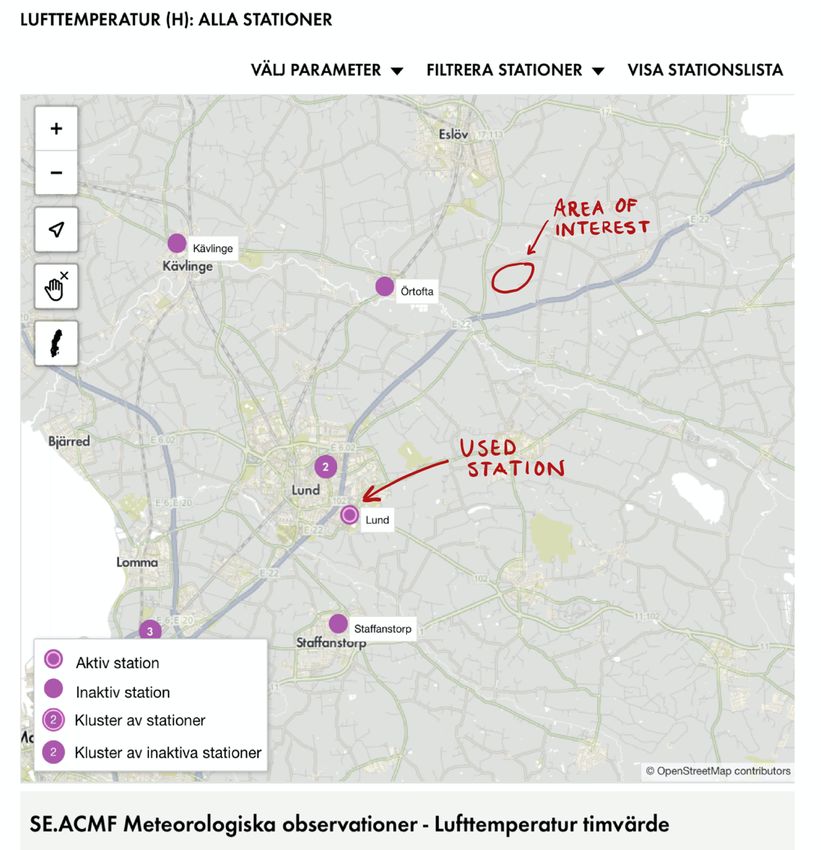
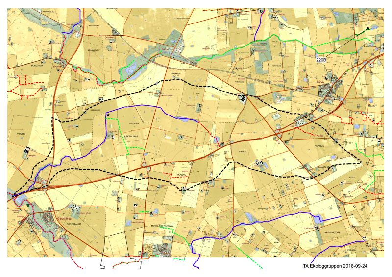
List of figures

FIGURE 1: MAP SHOWING THE POSITION OF GÅRDSTÅNGA NYGÅRD (VATTENATLAS
 2020). ..................................................................................................................... 3
FIGURE 2: MAP SHOWING THE SURFACE WATER IN THE AREA AROUND GÅRDSTÅNGA
 NYGÅRD, RÖDABÄCK IS MARKED IN RED (VATTENATLAS 2020). ........................... 4
FIGURE 3A & 3B: PICTURES OF THE SAME LOCATION IN RÖDABÄCK TAKEN DURING
 APRIL 2020 (LEFT) AND DURING MAY 2020 (RIGHT). ............................................. 5
FIGURE 4A & 4B: PICTURES SHOWING THE DIFFERENCE IN VEGETATION AND WIDTH IN
 TWO DIFFERENT LOCATIONS IN RÖDABÄCK DURING THE SAME DAY (BOTH
 TAKEN IN APRIL 2020). ........................................................................................... 5
FIGURE 5A & 5B: PICTURE OF OUTLET FROM PIPE TO RÖDABÄCK TAKEN IN MAY OF
 2020 (LEFT) AND MAP WITH LOCATION OF PIPE OUTLET MARKED WITH AN
 ARROW (RIGHT) (VATTENATLAS 2020). ................................................................. 6
FIGURE 6A & 6B: PICTURE OF THE POND TAKEN IN MAY OF 2020 (LEFT) AND MAP WITH
 LOCATION OF POND MARKED WITH AN ARROW (RIGHT)(VATTENATLAS 2020). .. 7
FIGURE 7A, 7B & 7C: PICTURE OF THE POND TAKEN IN MAY OF 2020 (LEFT), PICTURE
 OF THE POND TAKEN IN MARCH 2020 (MIDDLE) AND MAP WITH LOCATION OF
 POND MARKED WITH AN ARROW (RIGHT)(VATTENATLAS 2020). ......................... 8
FIGURE 8: THE LOCATIONS FROM WHICH WATER SAMPLES WERE TAKEN AND
 TEMPERATURE WAS MEASURED ON SITE (VATTENATLAS 2020). ........................ 18
FIGURE 9: THE LOCATIONS FROM WHICH THE WATER DISCHARGE WAS MEASURED
 (VATTENATLAS 2020). .......................................................................................... 20
FIGURE 10: ILLUSTRATION OF THE MEASURING OF WATER LEVELS IN THE CROSS
 SECTION NOT MADE TO SCALE. ............................................................................ 21
FIGURE 11: ILLUSTRATION OF SETUP FOR THE FLOAT METHOD NOT MADE TO SCALE. 22
FIGURE 12: THE DIFFERENCE IN VALUE BETWEEN PET (LINES) AND AET (BARS) FOR
 EACH MONTH (MONTHLY AVERAGES) IN A LOCATION IN SOUTHERN SWEDEN. A
 MAP SHOWING THE LOCATION RELEVANT FOR THE FIGURE IS INCLUDED IN
 APPENDIX 10 (BRANDT AND GRAHN (1998)). ...................................................... 30
FIGURE 13: LOCAL WATER FLOW IN KÄVLINGEÅN (THE CATCHMENT SHOWN IN
 APPENDIX 8) FOR EACH MONTH OF 2017 AND MONTHLY MEAN FLOW (SMHI
 2020). ................................................................................................................... 33

 xii

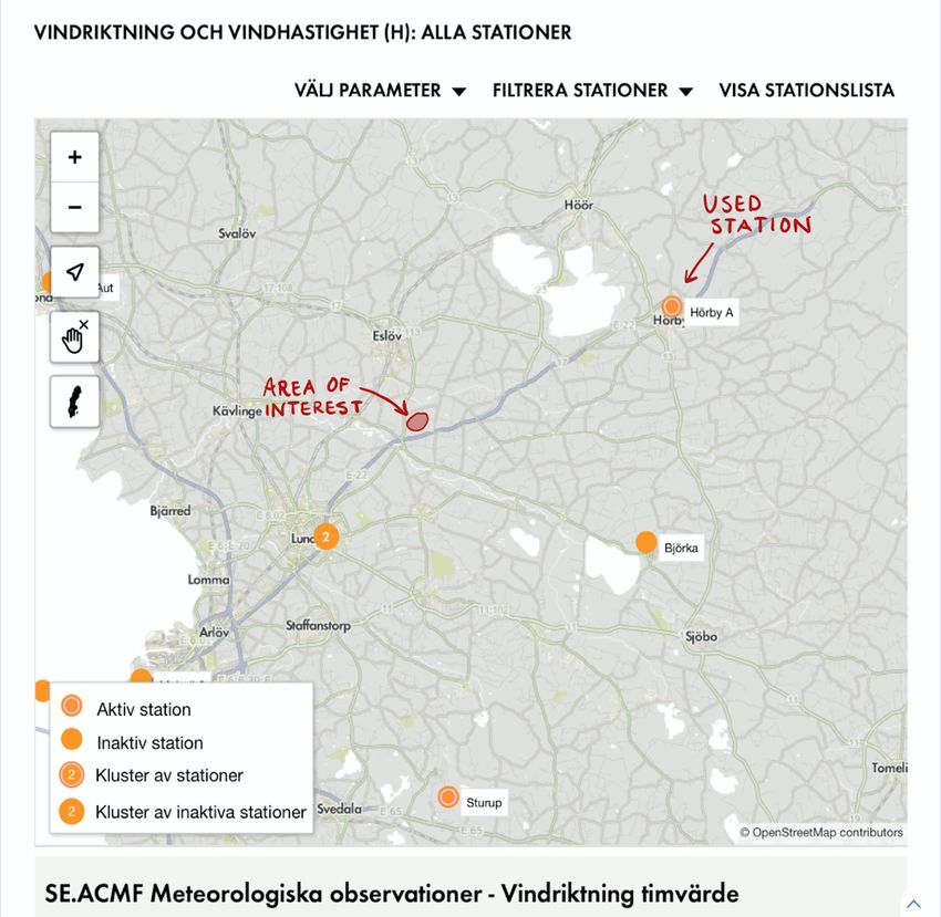
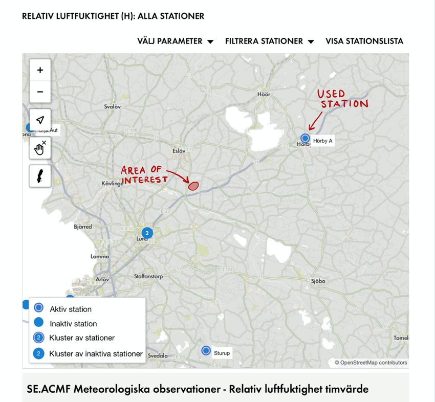
FIGURE 14: LOCAL WATER FLOW IN KÄVLINGEÅN (THE CATCHMENT SHOWN IN
 APPENDIX 8) FOR EACH MONTH OF 2018 AND MONTHLY MEAN FLOW (SMHI
 2020). ................................................................................................................... 33
FIGURE 15A & 15B: ILLUSTRATIONS OF SETUPS FOR MEASURING WATER LEVEL IN PIPE
 (LEFT) AND IN STREAM (RIGHT) NOT MADE TO SCALE......................................... 36
FIGURE 16: DIAGRAM SHOWING THE CROSS SECTIONAL AREA OF ONE PLACE IN
 RÖDABÄCK............................................................................................................ 41
FIGURE 17: THE CATCHMENT OF RÖDABÄCK WITH MARKING OF THE FUTURE
 CONSTRUCTED WETLAND IN THE SHAPE OF A STAR (ALSTRÖM 2020). ............... 56
FIGURE 18: THE SHAPE AND POSTION OF THE FUTURE CONSTRUCTED WETLAND.
 (ALSTRÖM 2020). ................................................................................................. 57
FIGURE 19: MAP SHOWING FROM WHICH ONE OF SMHI´S WEATHER STATION DATA
 ABOUT AIR TEMPERATURE WAS COLLECTED. (SWEDISH METEOROLOGICAL AND
 HYDROLOGICAL INSTITUTE 2020)......................................................................... 60
FIGURE 20: MAP SHOWING FROM WHICH ONE OF SMHI´S WEATHER STATION DATA
 ABOUT CLOUDINESS WAS COLLECTED. (SWEDISH METEOROLOGICAL AND
 HYDROLOGICAL INSTITUTE 2020)......................................................................... 61
FIGURE 21: MAP SHOWING FROM WHICH ONE OF SMHI´S WEATHER STATION DATA
 ABOUT RELATIVE HUMIDITY WAS COLLECTED. (SWEDISH METEOROLOGICAL AND
 HYDROLOGICAL INSTITUTE 2020)......................................................................... 62
FIGURE 22: MAP SHOWING FROM WHICH ONE OF SMHI´S WEATHER STATION DATA
 ABOUT WIND SPEED WAS COLLECTED. (SWEDISH METEOROLOGICAL AND
 HYDROLOGICAL INSTITUTE 2020)......................................................................... 63
FIGURE 23: SUBCATCHMENT OF KÄVLINGEÅN WHICH INCLUDES THE CATCHMENT OF
 RÖDABÄCK (SEE APPENDIX 1) (SWEDISH METEOROLOGICAL AND HYDROLOGICAL
 INSTITUTE 2020). .................................................................................................. 64

 xiii

1. INTRODUCTION

The agricultural industry has always been dependent on the availability of
water, and as earth is facing an increase in temperature the Swedish Board of
Agriculture (2020) is saying that the water needs of farms all around the world
will increase. The Swedish Board of Agriculture (2020) emphasizes that the
north of Europe probably will not be the region most affected by the rise in
temperature, however, farms in the north of Europe are still wise to look over
the way in which they manage water resources. Two aspects relevant to
agricultural water resource management is the way in which water is managed
with regard to water quantity and the way in which water is managed with
regard to water quality.
 Gårdstånga Nygård is a farm located in southern Sweden that at the
time of writing is in the process of upgrading the way in which water resources
are managed.

 1

1.1 Purpose

The purpose of this bachelor’s degree project is to measure, calculate and
compile data about aspects relevant to the water at Gårdstånga Nygård, and
therefore to evaluate to which extent the agricultural activities at Gårdstånga
Nygård is impacting the water quality of adjacent surface water bodies. The
project also includes a discussion about how adjacent surface water bodies will
be impacted by the planned future water management system of Gårdstånga
Nygård. The discussion will be based on estimated future data about water
quantity in the surface water bodies in the area. The project is aimed at
answering the following questions:

 • How is the water quality in Rödabäck and other water bodies about
 Gårdstånga Nygård and how is the water quality thought to be affected
 by the nearby agricultural activities?

 • Is there enough water available in the catchment for it to be justifiable
 to build a wetland within it?

 2

2. Theoretical background

2.1 Gårdstånga Nygård

Gårdstånga Nygård is a limited company operating agricultural activity on 900
hectares of land (Andersson 2017) in the municipality of Eslöv which is located
northeast of the city of Lund, Sweden. The blue marker in Figure 1 shows the
position of Gårdstånga Nygård.

Figure 1: Map showing the position of Gårdstånga Nygård (Vattenatlas 2020).

2.1.1 Current water management system

The area that is relevant to the project is subcatchment of the larger catchment
of the – compared to Rödabäck – large river called Kävlingeån. The bodies of
water within the subcatchment are all part of the water management currently
(as of spring 2020) present in and around the farmland managed by Gårdstånga
Nygård. Rödabäck´s catchment, namely the previously mentioned
subcatchment, is shown in appendix 1. In Figure 2 a map which includes the

 3

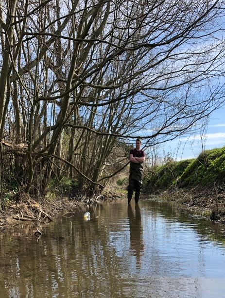
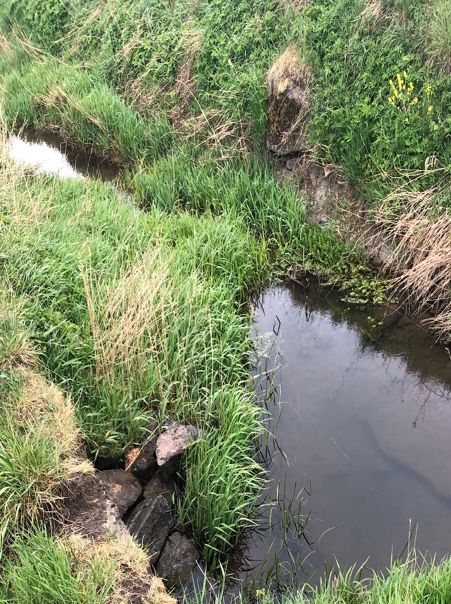
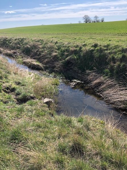
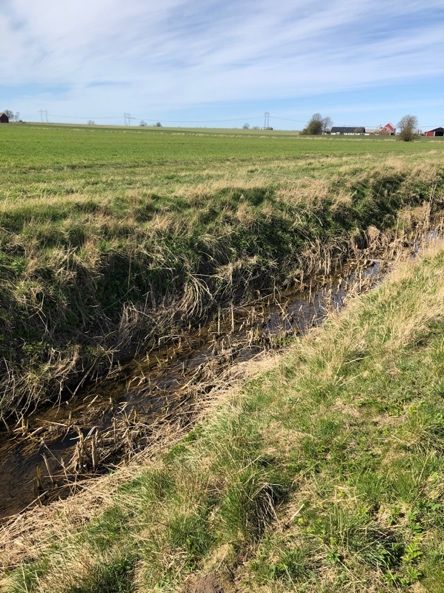
subcatchment is shown. In the map Rödabäck is marked out with red. The
features of the water management system around Gårdstånga Nygård that are
the most relevant to the project are highlighted later in this section of the report
(note that these are not the only water management features present in the area).

Figure 2: Map showing the surface water in the area around Gårdstånga Nygård, Rödabäck is
marked in red (Vattenatlas 2020).

Rödabäck is a stream with an estimated width of about 3.5 meters or less (this
estimation is supported by on site measurements). The stream is situated in the
midst of many fields that house agricultural activities in the form of plant
cultivation. The width and depth of the stream and the appearance of the
vegetation around the stream varies depending on season and where along the
stream the stream is observed. Figures 3a and 3b show examples of how the
same place in the stream looks different in terms of vegetation depending on
time of year. In Figures 4a and 4b examples of the differences in width and
vegetation are shown.

 4

Figure 3a & 3b: Pictures of the same location in Rödabäck taken during April 2020 (left) and
during May 2020 (right).

Figure 4a & 4b: Pictures showing the difference in vegetation and width in two different locations
in Rödabäck during the same day (both taken in April 2020).

 5

The dashed yellow line in Figure 2 represents an underground pipe which is
used for dewatering nearby farmland and then leading said water directly into
Rödabäck. The pipe has a diameter of 0.7 meters and its outlet into Rödabäck is
shown in a picture below along with a map showing the location of the outlet
(see Figures 5a and 5b). The area around the outlet was relatively heavily
vegetated during the spring of 2020.

Figure 5a & 5b: Picture of outlet from pipe to Rödabäck taken in May of 2020 (left) and map with
location of pipe outlet marked with an arrow (right) (Vattenatlas 2020).

In the map named Figure 6b, a pond located in the catchment is marked out, and
in Figure 6a it is shown how said pond looks. The pond functions as a detention
reservoir for some of the storm water passing through the subcatchment. The
area surrounding the pond, and also in the pond, a large amount of vegetation
was present throughout the spring of 2020. Trees line most of the perimeter of
the pond.

 6

Figure 6a & 6b: Picture of the pond taken in May of 2020 (left) and map with location of pond
marked with an arrow (right)(Vattenatlas 2020).

An additional pond serving as a detention reservoir is located nearby the
agricultural facilities of Gårdstånga Nygård. The position of this pond is marked
out in Figure 7c. Notice that this pond, unlike the pond previously mentioned, is
not directly connected to Rödabäck. Like the previously mentioned pond this
pond was relatively heavily vegetated throughout the spring of 2020.
Additionally, this pond’s water inlet was closed during some parts of the spring
of 2020. The inlet being closed resulted in a decrease in water flow, which is
thought to be the reason for the presence of a lot of organic matter gathering
around the whole inside perimeter of the pond –especially surrounding the inlet
– during the late spring of 2020 (see Figures 7a and 7b).

 7

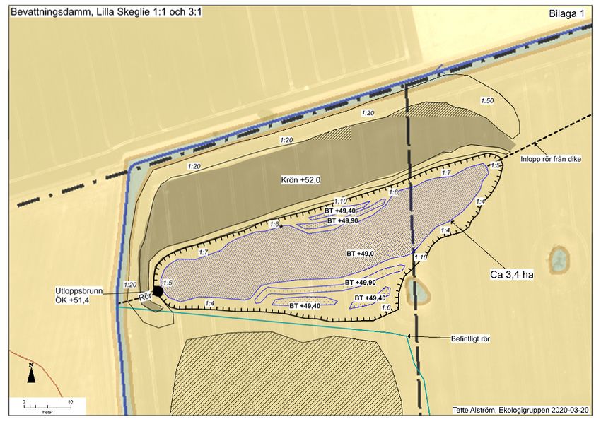
Figure 7a, 7b & 7c: Picture of the pond taken in May of 2020 (left), picture of the pond taken in
March 2020 (middle) and map with location of pond marked with an arrow (right)(Vattenatlas
2020).

2.1.2 Fertilization of agricultural fields during testing

According to the owner of Gårdstånga Nygård Gustaf Ramel (2020) a field
adjacent to Rödabäck was fertilized using 75 kg/ha of nitrogen and 10 kg/ha of
sulfur on March 7th of 2020. The field has an area of 58 ha.

2.1.3 Future constructed wetland

In the near future a new wetland will be constructed at Gårdstånga Nygård. The
planners of the wetland, Ekologigruppen, have expressed that the new wetland’s
main function will be to act as a reservoir for water that will later be used for
irrigation. The amount of water available for irrigation that the wetland will be
able to hold is 100 000 m3. Additionally, the planners have said that the new
wetland will be beneficial for nearby ecosystems and that the wetland will trap
nutrients traveling with the water in the wetland. (Alström, Tette 2020)
Appendix 2 shows how the new wetland will be positioned and shaped, and it
can also be read from the picture in appendix 2 that the wetland will have an
area of about 3.4 hectare. Appendix 1 shows the shape of the catchment of
Rödabäck, and the new wetlands’ position is also shown with a marker in the
shape of a star.

 8

2.2 Water quality

The requirements in order for the quality of water to be considered good is
different depending on what the water in question is going to be used for. Water
that is going to be used for irrigation for example, which is the case for the
water in the water bodies about Gårdstånga Nygård, cannot contain excessive
amounts of minerals because that could cause adverse osmotic processes
occuring in the plants. Having sufficient water quality in water courses is also
strongly correlated with the survival of plants and animals in the aquatic
ecosystems. The water bodies that are presented in the section called “2.1.1
Current water management system” of this report are, and will be in the future,
used as sources of water for irrigation and as habitat for various aquatic
organisms, and for this it is of great importance that these water bodies maintain
a high water quality. (Boyd 2020, p.ix)
 In the remainder of this section (2.2 Water Quality) some problems
related to water quality in an agricultural setting and some of the parameters that
can be used to indicate the existence of these problems will be exhibited.

2.2.1 Agricultural leaching

Agricultural leaching is a natural process occurring in soil used in agriculture
when it’s exposed to irrigation and rain. When leaching occurs the water that is
being transported through the soil interacts with the surfaces of different kinds
of materials in the soil. (Swedish National Encyclopedia (n.d.)) Easily
accessible parts of these materials are then dissolved and carried away with the
water. The physical movement of water that occurs in conjunction with
agricultural leaching can also result in larger particles being moved by the
water. When compounds and larger particles have been made mobile by the
water they are likely to be transported out of the Critical Zone, which means
that the compounds and larger particles that are or consist of nutrients can no
longer be beneficial for agricultural crops and are likely to affect the
surrounding environment in a negative way, namely by increasing the rate of
eutrophication in bodies of water. (Richardson 2016) Phosphorus and nitrogen

 9

are both substances that often reach bodies of water as a result of fertilization of
land in an agricultural setting and the leaching of said land, and the amount of
phosphorus and nitrogen in a body of water is a good parameter to take into
account when assessing the water quality in said body of water. (United States
Geological Survey (n.d)) The way in which the amount of phosphorus and
nitrogen affects water quality is illustrated in greater detail under the heading
“Phosphorus, nitrogen, total organic carbon and eutrophication”.
 Beyond nutrient leaching it is also important to consider the importance
of salt leaching in agriculture. Too much salt in the Critical Zone can impact
crops in a significantly negative way, which means that leaching is necessary in
agriculture. In order to avoid too much nutrients and too little salt being
transported from the soil the irrigation must be carried out in an appropriate
way. (Richardson 2016) Salt leaching is also relevant to take into account when
assessing water quality, and parameters that can be used for this are dissolved
solids and electrical conductivity (Boyd 2020, p.84). The reason for why it is
relevant to measure these parameters when assessing water quality is explained
under the header “Dissolved solids and electrical conductivity”.

2.2.2 Dissolved solids and electrical conductivity

Dissolved solids and electrical conductivity are both indicators of salinity in
water which makes them both relevant parameters when assessing water quality.
(Boyd 2020, p.84) The quantification of to which extent a material conducts or
resists electric currents is called the material’s electrical conductivity. Electrical
conductivity is measured in a unit called Siemens (S). The conductivity of water
is strongly correlated with the amount of ions that are dissolved in the water,
which is why measuring conductivity is a good way of estimating the salinity of
water samples. (Swedish National Encyclopedia (n.d.)) Extensive deviations in
conductivity from what is considered the normal conductivity is an indicator
that some kind of disturbance has affected the water course, which means that
looking for change in the degree of conductivity in water is a good way of
discovering whether some kind of disturbance, for example a disturbance

 10

created by nearby agricultural activity, has affected the water course in some
point of time (United States Environmental Protection Agency (n.d.)).
 Solids that are dissolved in water consist of inorganic material, namely
minerals, and organic material. Most of the dissolved solids in water are often
minerals which is why waters with a high amount of dissolved solids are said to
be highly mineralized. In order to be drinkable for humans the amount of
dissolved solids in water should not exceed 550 mg/L, but it is normal for
freshwater to contain as much as 1000 mg/L of dissolved solids. (Boyd 2020,
p.84)

2.2.3 Phosphorus, nitrogen, total organic carbon and
eutrophication

High concentrations of phosphorus and nitrogen in water bodies usually result
in eutrophication, and high concentrations of phosphorus and nitrogen is often a
result of activities carried about by humans, such as fertilizer being used in an
agricultural setting. (Boyd 2020, p.308, 289)
 Eutrophication is the development towards an environment in a body of
water that is richer in nutrients, which leads to an increase in the growth rate of
algae and aquatic plants. The increased amount of algae and plants in the body
of water means that there is an increase in the amount of organic material (also
known as total organic carbon) present (Swedish Environmental Protection
Agency 2019), which then leads to a decrease in water quality, namely a
decrease in the amount of dissolved oxygen present (Swedish National
Encyclopedia (n.d.)). The significance of dissolved oxygen in bodies of water is
illustrated in detail under the heading called “Dissolved oxygen”.
 To gain perception about if and to which extent human influence affects
a body of water, measurement of phosphorus content, nitrogen content and total
organic carbon (also known as organic material) can be carried out. By
measuring these parameters both upstream and downstreams from a suspected
source of pollution one can determine whether the suspected source of pollution
is a source of pollution. (Carrow, Duncan and Huck 2009) Note that agricultural
activities can be a direct source of phosphorus, nitrogen and organic carbon, but

 11

that the quantity of organic carbon in a body of water can be enlarged even
further as a result of the presence of nitrogen and phosphorus (Swedish
Environmental Protection Agency 2019). Phosphorus levels in fresh water is
generally lower than 0.5 mg/L (Boyd 2020, p. 302). It is normal for the total
nitrogen in streams flowing through farmland to reach values of 2 mg/L to 15
mg/L and over (Ekologgruppen i Landskrona AB 2014), whereas the total
nitrogen in freshwater that does not flow through farmland, that is relatively
unpolluted water, generally does not exceed 2 mg/L (Boyd 2020, p. 287).

2.2.4 Dissolved oxygen

The existence of dissolved oxygen in water, in the form of molecular oxygen, is
essential for all aerobic organisms living in water. Beyond the fact that enough
oxygen being dissolved in water is important to the respiration of aquatic
organisms, levels of dissolved oxygen that are too high can be deadly to
organisms living in the water. (Boyd 2020, p.6-7) An acceptable level of
dissolved oxygen in a shallow water course such as Rödabäck is 4-15
milligrams per litre. 4-15 milligrams per litre of dissolved oxygen constitutes a
dissolved oxygen level high enough for aquatic life to thrive in shallow waters.
 Dissolved oxygen in water has a correlation with the temperature of
said water, namely the same water sample that has one value for dissolved
oxygen at 5℃ has a lower value for dissolved oxygen at 10℃. (Fondriest
2013a)
 Oxygen is dissolved in water through the photosynthesis of plants
inhabiting the water or by being diffused into the water through the atmosphere.
The rate in which oxygen dissolves into water is dependent on the amount of
dissolved oxygen already present in the water, the size of the contact area
between the water and the air and turbulence level of the water. (Boyd 2020,
p.6-7)

 12

2.2.5 Turbidity and suspended solids

Both suspended solids and turbidity are parameters related to the the amount of
particles present in water, the difference between them is that turbidity is a
parameter measuring the water clarity, namely it expresses to which extent light
travels through water (which depends on the amount of solids in the water),
whereas suspended solids is a parameter directly related to amount of particles
in the water.
Clear bodies of water, namely bodies of water with a low turbidity and a low
amount of suspended solids are usually considered healthier than bodies of
water with a high turbidity and a high amount of suspended solids. Note that it
is possible for a water course with what is considered a low clarity and a high
amount of suspended solids to be healthy, and a sudden change in the clarity
and the amount of suspended solids in a water course is greater cause for
concern than a water course with a consistently high level of turbidity and
amount of suspended solids.
 A sudden increase in turbidity and suspended solids is often caused by
human influence such as pollution from wastewater treatment plants or
agriculture. Activities that include disturbing areas by loosening soil, such as
construction and agriculture, also increase the probability that nearby water
bodies see an increase in turbidity and suspended solids. Animal waste and
fertilizers are transported into water courses from farms unintentionally with
runoff and sometimes intentionally with discharge, which causes increased
turbidity and amount of suspended solids, increased pathogen concentration and
eutrophication. Tilling, also an activity often carried out in conjunction with
agriculture, increases the amount of erosion in the soil, which leads to an
increase in soil particles reaching the water courses and raising the turbidity and
amount suspended solids, therefore causing disturbances in aquatic ecosystems.
 The amount of suspended solids in a water course having a value below
20 milligrams per litre and the turbidity having a value below 55 NTU usually
means that the water course in question is considered clear. (Fondriest 2014)

 13

2.2.6 pH

When measuring the acidity or the alkalinity of water pH is used. Water that is
considered safe for the majority of aquatic organisms has a pH level between
6.5-9.0. A pH level that is not within this range can cause a decrease in survival
rates of aquatic organisms and a change in the solubility of elements and
compounds, causing eutrophication and further disturbances in aquatic
ecosystems.
 Changes in pH can occur due to both human and natural influences.
Natural processes that can lead to changes in stream water pH include for
example lightning, nearby fires and the existence of sulfate-reducing bacteria in
wetlands. Man-made pH influencers include pollution related issues such as
acid rain and wastewater discharge. (Fondriest 2013b) The pH level of water in
inland waters is also correlated with the way in which the water in question has
traveled through the landscape and into the water course, pH in water is
generally lower if the water has infiltrated soil and higher if the water has
traveled overland. This is because water infiltration in the soil often results in
the water being charged with carbon dioxide, lowering the pH of the water.
(Boyd 2020, p.97)

2.2.7 Temperature

The conditions for aquatic life in a water course is dependent on the water’s
temperature. Temperature changes due to human influence may affect water
course habitants and perturb the natural competition between organisms living
in the water course. (Credit Valley Conservation 2020)

 14

2.3 Water quantity

2.3.1 Discharge flow

The cross sectional area of a stream multiplied with the velocity of the water in
the stream is the stream’s discharge flow. When assessing the characteristics
and quality of a water course it is very important to take the flow of water in the
water course into consideration. The flow in a water course affects the
concentration of substances in the water, the water temperature and the amount
of dissolved oxygen, sediment and suspended solids in the water. Which aquatic
organisms that live in a given water course is highly dependent on the flow of
said water course.
 The greatness of flow in a water course is dependent on the amount of
precipitation within the catchment of the water course, however the effects of
precipitation on water courses are more or less high depending on the vegetation
in the watershed and whether there are any ponds or wetlands nearby.
Vegetation, ponds and wetlands all prolong the time it takes for water to travel
into a water course, which means that existence of vegetation, ponds and/or
wetlands in a watershed lowers the maximum flow that the water in a
watercourse takes on because of a nearby rain- or snowfall. (Water On The Web
2020)

2.3.2 Water balance

The concept of a water balance is built upon the fact the existing water amount
is unchanging, meaning that all the water within earth’s atmosphere is part of
the hydrological cycle. By implementing the water balance equation (see the
section called “3.2.2 Water Balance”) one can gain information the availability
of water resources within in a specified area over a specified period of time.
(Abd-Alhadi et al. 2007)

 15

2.3.3 Water level

Because many water quality parameters depend on water
level, measuring water level is important to determine when assessing
water quality. (Credit Valley Conservation 2020)

 16

3. METHOD, MATERIALS & EXECUTION

The study consisted of both examining already existing data and of going to the
relevant site, the catchment of Rödabäck, and collecting new data.
 It is important to note that the investigation dealt with two different time
periods, the parts of the project that dealt with water quality and the part that
involved measuring the stream flow rate of Rödabäck is relevant to the spring of
2020, whereas the part of the report that dealt with water balance concerns any
year with what is considered extreme weather prerequisites. The reason that the
part about water quality and the part about measuring stream flow rate is
relevant to the spring of 2020 is that the spring of 2020 is the time period within
which the measurements for these parts were taken. The reason for that the
water balance calculations were done using data from 2017 and 2018 is
explained in section 3.2.2. The investigation concerning water quality and
stream flow rate in Rödabäck in the spring of 2020 were done in order to gain
perception about how the nearby agricultural activities are affecting the water
quality of Rödabäck, whereas the implementation of a water balance equation
could lead to a better understanding of availability of water in the catchment.

3.1 Assessing Water Quality

The assessment of water quality of the water in Rödabäck was done by first
identifying five locations of water from which data about water quality could be
used to draw conclusions about how the water quality in water courses about
Gårdstånga Nygård is being affected by the nearby agricultural activities. The
locations from which the water samples were taken are shown in Figure 8 in the
form of red rings:

 17

Figure 8: The locations from which water samples were taken and temperature was measured on
site (Vattenatlas 2020).

The respective locations shown in the figure are labeled with the letters A, C, E,
F and G, and those are names that will be used for the locations throughout the
report. Location A, C and E were considered places of interest because
conclusions about how the drainage pipe (shown in the Figure 8 as a dashed
dark yellow line) leading into Rödabäck at location C (see Figures 5a and 5b)
affects the water quality in Rödabäck downstream from the place of the outlet.
A comparison of the values assigned to the different water quality parameters in
locations A, C and E could lead to a better understanding about how the
drainage water coming into Rödabäck through the drainage pipe (which
dewaters a large area of nearby farmland) affects the water quality of the
stream.
 Location F is located in a pond that is connected to Rödabäck
downstream from the previously discussed locations (see Figures 6a and 6b). A
water quality assessment of water samples fetched from location F was included
because it was thought that it could be valuable when determining to which
extent the agricultural activities about Gårdstånga Nygård affects the local water
courses in general, and for non-flowing, stationary water in particular.

 18

A location further south compared to the previously mentioned location
is called location G, and is part of an additional pond (see Figures 7a, 7b and
7c). This location was included in the investigation because it is also part of a
pond in which drainage water from farmland is collected.
 The dates on which the water samples were collected were February
7th, March 3rd, March 27th, April 3rd and May 16th (all during the year of
2020). On the respective days one water sample from each previously
mentioned location was collected.

3.1.1 In field

Water samples from locations A, C, E, F and G were collected in plastic bottles
and later brought to laboratories to be tested. The water temperature of each
location was measured on site using a thermometer.

3.1.2 In the laboratory

The samples were stored in a refrigerator with a temperature of about 9 ℃ in the
lab before being tested. Firstly, the suspended solids, dissolved solids, dissolved
oxygen, turbidity, pH and conductivity of the collected water samples was
measured in the laboratory of the division of Water Resource Engineering at
Lund University. The conductivity and the amount of total dissolved solids was
measured using a Conductivity Meter CO 310 (VWR, Germany). The amount
of dissolved oxygen in the water samples was measured using a dissolved
oxygen meter, VWR® DO 220 model (VWR, International). The turbidity was
measured using a turbidity meter called Turb® 430 IR (VWR, Germany). The
pH was measured using a pHenomenal® pH1100L meter (VWR, Germany).
The total amount of suspended solids was measured using a Lovibond MD 100
(VWR, Germany).
The water samples were then sent to another laboratory to be tested for
phosphorus- (TP), nitrogen- (TN) and organic carbon (TOC) content.

 19

3.2 Assessing Water Quantity

3.2.1 Discharge flow

The volume flow rate of a stream was calculated through the following
equation:

 = ∙ (1)

 = [ ! / ]
 = [ " ]
 = [ / ]

Below it is explained how the data about velocity and cross sectional area was
collected during observations. The discharge flow was measured at two
locations. The first location at which the discharge flow was measured was in
the stream (see the bottom marking in Figure 9) and the second location was in
a pipe which was leading water into the stream (see the top marking in Figure
9).

Figure 9: The locations from which the water discharge was measured (Vattenatlas 2020).

 20

Measuring cross sectional area of the stream
To find the cross sectional area of the stream a measuring tape was spanned
horizontally across the watercourse. The water level was then measured in
intervals of 10 centimeters using a ruler, this process is illustrated in Figure 10.

Figure 10: Illustration of the measuring of water levels in the cross section not made to scale.

The water levels on the different places in the stream were recorded in
Microsoft Excel and then used to make a cross section diagram which was used
to calculate the area of the cross section.

Measuring velocity of water in the stream
In order to find the velocity of the water in the stream The Float Method was
used. A distance of 10 meters was measured and marked out along the stream.
An object was then placed at the start of the 10 meters (this location is marked
out in Figure 11) and was allowed to travel along the stream to the finish of the
10 meters. The time it took for the object to travel from the starting point to the
finishing point in the stream was recorded. The placing of the object and
measuring of its travel time was repeated three times.

 21

Figure 11: Illustration of setup for The Float Method not made to scale.

The collected data of the object’s travel time was then used to calculate the
average travel time for the specific location using Eq. (2).

 1 + 2 + 3
 ̅ = (2)
 3

The calculated average travel time was used to calculate velocity of the stream.

 &
 = (3)
 '

 = = 10 

Determining discharge flow in pipe
The discharge flow in the pipe was measured using the same method that was
used when measuring the discharge flow of the stream, however the cross
section area of the water in the pipe was calculated using the diameter of the
pipe d, the water level in the pipe and the equation for calculating a segment of
a circle:

 22

($ )
 = "
 (*+, − sin ) (4)

 = 
 = ℎ 

The traveled distance l was set to 0.6 meters when measuring velocity of the
water in the pipe.

 23

3.2.2 Water balance

Data from two different years was used in order to examine how the amount of
water stored in the soon to be constructed wetland (see appendix 2) could vary
depending on the amount of precipitation occurring. The two years from which
data was used is 2017 and 2018 and the reasoning behind choosing these two
years was that 2017 was an unusually wet year in terms of precipitation and
2018 was an unusually dry year in terms of precipitation. Precipitation data
from 2017 and 2018 does well in representing a spectrum in which the amount
of precipitation varies in the relevant area. The following equation was used
when calculating the water balance:

 = + + ± ∆ ± ∆ (5)

 = [ ]
 = [ ]
 = [ ]
∆ = ℎ [ ]

There is assumed to be no subsurface flow across the watershed.
 , ∆ = 0

In the sections below it is explained how the factors used in the water balance
were produced.

Precipitation
Data concerning precipitation in the area in the years 2017 and 2018 was found
through the website of the Swedish Meteorological and Hydrological Institute
(SMHI) on April 15th 2020. In Table 1 the precipitation data for each month
during 2017 and 2018 is reported.

 24

Table 1: Approximated precipitation within the catchment for each month of 2017 and 2018
(SMHI)

 Month
 Jan Feb Mar Apr May Jun Jul Aug Sep Oct Nov Dec
 %&'(
 27.7 64.3 46.0 45.2 33.4 112.3 58.1 55.7 111.1 90.1 70.3 70.3
 [mm]
 %&')
 55.6 29.7 55.2 34.4 2.3 18.1 2.5 90.7 32.4 56.1 27.0 73.1
 [mm]

The data from 2017 and 2018 respectively shown in Table 1 was used to
calculate the total precipitation for the whole years of 2017 and 2018.

 '-',",*/ = 784.5 
 '-',",*+ = 477.1 

Potential evapotranspiration
The penman formula was used to approximate the potential evapotranspiration
from Rödabäck and a document supplied by Lund University’s Faculty of
Engineering was used as a guide through the calculating process. The potential
evapotranspiration (PET) was calculated using the following equation:

 ∆
 012,
 = + ∆ (6)
 1*
 +

During the process of calculating the potential evapotranspiration it was
necessary to use the website of SMHI to retrieve data about air temperature,
wind speed, cloudiness and relative humidity. Because all SMHI stations with
which they measure various parameters do not all measure air temperature, wind
speed, cloudiness and/or relative humidity it was not possible to rely on one
station to retrieve all the data needed to do the calculations.
 Firstly, data about temperature 3 was found using the website of
SMHI, a map included in appendix 4 shows which measuring station was used
to retrieve data about the temperature. The temperature data for each month is

 25

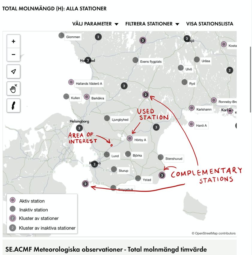
an average of all the data that was recorded that month. When the monthly mean
 ∆
air temperature had been made available the empirical parameter could be
 5
determined using one of the tables in the document supplied by the faculty. The
 ∆
values for 5 and 3 are included in appendix 3.
 The energy budget H was calculated using equations (7), (8), (9), (10)
and (11):

 = (1 − ) 67 − - (7)
 (1 − ) 67 = 0.95 3 (0.18 + 0.55 / ) (8)
 - = 38 (0.56 − 0.09\ 9 )(0.10 + 0.9 / ) (9)
 / = 1 − (10)
 9 = ∙ 3 (11)

The incoming radiation 67 is calculated using Eq. (8) and the parameters 3 , r
and n/N. The value of the albedo r is 0.05. 3 is the solar radiation and its value
depends on the latitude of the relevant location, latitude 60 in this case, and
which time of the year it is. The value of 3 was retrieved from the document
supplied by the faculty, and the values of 3 that were used in the calculations
are attached in appendix 3.
 n/N describes the ratio between the actual sunshine hours and the
possible sunshine hours. Data that was used to calculate the value of n/N was
found through the website of SMHI. The data that was retrieved from SMHI in
order to calculate n/N was data about cloudiness. How n/N is calculated from
the cloudiness is shown in Eq. (10). All the recorded data that was available was
used to calculate a monthly mean cloudiness. When retrieving the data about
cloudiness it was discovered that using only the station closest to the catchment
was not enough, this was because that station had malfunctioned during two
long periods of time during 2017 and 2018. Because of this, three other stations
were used as complement to the first station and for the months in which the
first station had malfunctioned the mean monthly cloudiness was calculated by
finding the average of the cloudiness for the three complement stations. The
values for n/N that was used in further calculations are reported in appendix 3
and a map showing from which stations the data was collected is attached in

 26

appendix 5, in appendix 3 it is also indicated which monthly mean values were
calculated using several stations. The values for the incoming radiation 67 that
were found using 3 , r and n/N are attached in appendix 3.
 The outgoing radiation - was calculated using Eq. (9). 38 the
theoretical black body radiation and its value was found in the document
supplied by the faculty using the previously mentioned monthly mean air
temperature 3 . The values of the black body radiation for each month used in
the calculations are attached in appendix 3.
 The actual vapor pressure edwas calculated using Eq. (11). The relative
humidity RH is found through the SMHI website and the saturation vapor
pressure 3 was found through the document supplied by the faculty. The values
of 9 , 3 and RH that were used in the calculations are included in appendix 3
and a map showing the locations of the station that were used to measure RH are
included in appendix 6. The values for the outgoing radiation - that were
found using 38 , n/N and 9 are attached in appendix 3. The values for the
energy budget H are included in appendix 3.
 The mass transfer 3 was calculated using the equation below:

 $:
 3 = 0.35(0.5 + *,, ( 3 − 9 ) (12)

The way in which the parameters 9 and 3 were found is explained in earlier
parts of the text. " is the wind speed and it’s values were found through SMHI.
The mean monthly sizes of the wind speed in the area are reported in appendix
3. A map showing the location of the station from which the data about wind
speed was collected is also included in appendix 7. The values of the mass
transfer 3 for the various months is included in a table in appendix 3.
 In Table 2 the approximated potential evapotranspiration is reported and
the values were calculated using Eq. (6). Note that in the case of January,
November and December in 2017 and March and November in 2018 the
potential evapotranspiration was set to 0 millimeters per day. In the case of
March of 2018 the potential evaporation was set to 0 because the monthly
average temperature 3 was below 0℃ which meant that the evapotranspiration
was negligible. The potential evapotranspiration of January, November and
December in 2017 and November in 2018 was set to 0 millimeters per day

 27

because the calculations showed a negative value for the potential
evapotranspiration which meant that the potential evapotranspiration in those
cases also was negligible.

 28

Table 2: Potential evapotranspiration within the catchment for each month of 2017 and 2018.

 Month
 Jan Feb Mar Apr May Jun Jul Aug Sep Oct Nov Dec
 %&'(
 0.0 4.7 19.5 51.1 97.2 117.9 112.2 77.1 42.8 16.9 0.0 0.0
 [mm]
 %&')
 0.7 4.8 0.0 47.0 114.9 134.3 143.4 98.8 54.9 16.0 0.0 0.5
 [mm]

The data from 2017 and 2018 respectively shown in the Table 2 was then used
to calculate the actual evapotranspiration (AET) the process of which is shown
later in the report.

Actual evapotranspiration
The actual evapotranspiration AET was calculated using the equation (Allen et
al. 1998, ch. 6) below:

 = ; ∙ (13)

 = [ ]
 < = [−]

The crop coefficient that was used for calculating the actual evapotranspiration
of each of the months of 2017 and 2018 is a rough estimate based on a report
published by SMHI and an average crop coefficient during March and until the
end of September produced via hydrological modelling with a value of 0.637
(Persson, M. 2020). In the previously mentioned report published by SMHI
Figure 12 can be found:

 29

Figure 12: The difference in value between PET (lines) and AET (bars) for each month (monthly
averages) in a location in southern Sweden. A map showing the location relevant for the figure is
included in appendix 10 (Brandt and Grahn (1998)).

Figure 12 was used to approximate the way that the crop coefficient varies
throughout a year. The monthly average crop coefficient for the months March-
September in the case shown in figure 12 was calculated to 0.65, and because
of the similarity between this value and the average crop coefficient produced
via hydrological modelling (0.637) the information displayed in figure 12 was
marked as usable for approximating the crop coefficient for each month of the
year. Note that time period of which Figure 12 is based is 1961-1990, namely
not the same time period for which the water balance was calculated. The
following table shows the crop coefficient for each month approximated using
figure 12:

Table 3: Approximated crop coefficient for each month of a year.

 Month
 Jan Feb Mar Apr May Jun Jul Aug Sep Oct Nov Dec

 - [-] 0.95 0.20 037 0.91 0.92 0.64 0.58 0.55 0.59 0.91 0.95 0.95

 30

The approximated actual evapotranspiration could then be calculated using Eq.
(13) and tables 2 and 3. The approximated actual evapotranspiration for each
month is shown in table 4:

Table 4: Actual evapotranspiration within the catchment for each month of 2017 and 2018.

 Month
 Jan Feb Mar Apr May Jun Jul Aug Sep Oct Nov Dec
 %&'(
 0.0 0.9 7.2 46.5 89.5 75.4 65.1 42.4 25.3 15.4 0.0 0.0
 [mm]
 %&')
 0.7 1.0 0.0 42.8 105.8 85.9 83.2 54.4 32.4 14.5 0.0 0.5
 [mm]

The monthly values can then be used to calculate a yearly value for actual
evapotranspiration for 2017 and 2018:

 '-',",*/ = 367.7 
 '-',",*+ = 420.9 

Runoff
Because data about the surface runoff in the catchment was not available a
approximation of monthly values for the surface runoff R was made by first
calculating a total yearly value of R for 2017 and 2018 using Eq. (5). In Eq. (14)
it is shown how Eq. (5) can be modified when considering a water balance on a
yearly basis.

 '-' = '-' + '-' (14)

The term for change in storage ∆ is not shown because it is typically
nonexistent over a time period of one year. The calculated values for P year and
AET year are displayed earlier in the text and they can be used to calculate the
yearly runoff in 2017 and 2018.

 '-',",*/ ≈ 2893.2 

 31