COVID-19 infection data encode a dynamic reproduction number in response to policy decisions with secondary wave implications
←
→
Page content transcription
If your browser does not render page correctly, please read the page content below
COVID-19 infection data encode a dynamic
reproduction number in response to policy
decisions with secondary wave implications
Michael A. Rowland ( michael.a.rowland@usace.army.mil )
U.S. Army Engineer Research & Development Center
Todd Swannack
U.S. Army Engineer Research & Development Center
Michael L. Mayo
U.S. Army Engineer Research & Development Center
Matthew Parno
U.S. Army Engineer Research & Development Center
Matthew Farthing
U.S. Army Engineer Research & Development Center
Ian Dettwiller
U.S. Army Engineer Research & Development Center
Glover George
U.S. Army Engineer Research & Development Center
William England
U.S. Army Engineer Research & Development Center
Molly Reif
U.S. Army Engineer Research & Development Center
Jeffrey Cegan
U.S. Army Engineer Research & Development Center
Benjamin Trump
U.S. Army Engineer Research & Development Center
Igor Linkov
U.S. Army Engineer Research & Development Center
Brandon Lafferty
U.S. Army Engineer Research & Development Center
Todd Bridges
U.S. Army Engineer Research & Development Center
Research Article
Page 1/12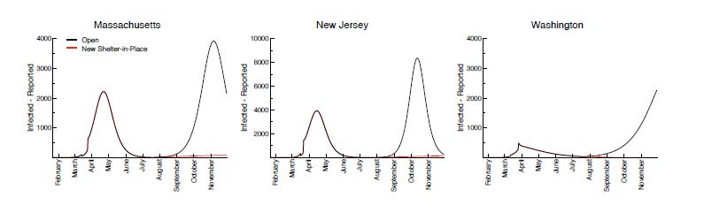
Keywords: modeling, simulations, COVID-19
DOI: https://doi.org/10.21203/rs.3.rs-75665/v1
License: This work is licensed under a Creative Commons Attribution 4.0 International License.
Read Full License
Page 2/12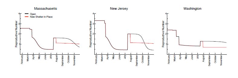
Abstract
The SARS-CoV-2 virus is responsible for the novel coronavirus disease 2019 (COVID-19), which continues
to spread to populations throughout the continental United States. Most state and local governments
have adopted some level of “social distancing” policy, but infections have continued to spread despite
these efforts. Absent a vaccine, authorities have few other tools by which to mitigate further spread of the
virus. This begs the question of how effective social policy really is at reducing new infections that, left
alone, would likely overwhelm the existing hospitalization capacity of many states. We developed a
mathematical model that captures correlations between state-level “social distancing” policies and
infection kinetics for all U.S. states, and use it to illustrate the link between social policy decisions,
disease dynamics, and an effective reproduction number that changes over time, for case studies of
Massachusetts, New Jersey, and Washington states. In general, our ndings indicate that the potential for
second waves of infection, which result after reopening states without an increase to immunity, can be
mitigated by a return of social distancing policies as soon as possible after the waves are detected.

Introduction
The virulent SARS-CoV-2 virus is responsible for the pandemic of novel coronavirus dis- ease 2019
(COVID-19) currently a icting the global population. The rst con rmed instance of COVID-19 in the
United States was recorded on 21 January 2020; since then, total reported in- fections have soared to
4,363,511 con rmed cases and over 149,375 deaths in the United States as of 29 July 2020 [1, 2] . By
March 2020, relatively few forecasting tools were available for relia- bly estimating trends in reported
infections [3, 4] . This led to a level of uncertainty in the e cacy of social policy to control the rate of
further infections in both urban and rural populations. At a federal level, the United States Army Corps of
Engineers (USACE), Federal Emergency Manage- ment Agency (FEMA), and the Department of Health &
Human Services have responded to the COVID-19 pandemic with domestic relief efforts [5] , but these are
primarily reactive and localized to existing outbreak hotspots. Limitations in the availability of personal
protective equipment (e.g., N95 masks) and critical care tools (e.g., ventilators) require a more proactive
approach to understanding where and when the most severe outbreaks will occur. The largely unknown
e - cacy of social policy to reduce the interactions between infected and susceptible individuals that lead
to new COVID-19 infections makes a proactive approach especially important. Even more uncertain is the
potential for sequestered yet susceptible individuals to fuel a “second wave” of infections. Therefore, we
can expect that the timing of social distancing policies will correlate with future infection waves through
population immunity, other dynamic features of population movement, and accessibility to infected
individuals. Here we report on efforts to deduce these dependencies from infection data reported by the
health departments of Massachusetts, New Jersey and Washington—states with extensive, early COVID-
19 outbreaks—by developing new methods capable of adapting to and anticipating dynamic trends in a
diurnally updated time se- ries, using a tool we refer to as the Engineer Research & Development Center
Susceptible-Ex- posed-Infected-Recovered (ERDC SEIR) model.
                                                    Page 3/12
Methods
Data acquisition
Available COVID-19 datasets primarily represent data aggregated from the individual re- ports of state
health departments and are made publicly available by several organizations, most notably by the Johns
Hopkins University (JHU) [1] and USAFacts (https://usafacts.org/visualiza- tions/coronavirus-covid-19-
spread-map/). We chose to use the USAFacts datasets that report COVID-19 cases for all 3,141 counties
and parishes of the United States, whereas the JHU datasets report a mixture of municipalities and
multiple scales (state and county) in addition to a selection of foreign locations. The USAFacts datasets
represent the cumulative number of positive COVID- 19 cases reported over time. As the pandemic
proceeds across the United States, we should therefore expect these data to represent trends that rise
exponentially with the rst COVID-19 reports to plateau when the infection wanes. The in ection point of
this cumulative reported infection curve therefore represents the peak in new daily reported infections.
There are several unique challenges associated with modeling COVID-19 infection data. First, datasets
are continually updated to include new reports that serve to reduce the uncer- tainty in infectious trends
as the disease progresses with time. Second, there are few studies informing key epidemiological
parameters that help to model progression of COVID-19 in suscep- tible populations, leading to greater
uncertainty surrounding values for the latency period (3-10 days), Z, or the duration of symptoms (5-14
days), D [6-8]. Other challenges exist, such as wide- spread testing delays that potentially contribute to a
sampling bias in the available data [9]. SARS- CoV-2 is an RNA virus, meaning that reverse transcription
polymerase chain reaction (RT-PCR) testing is required to detect the presence of virus in samples [10]. The
RT-PCR testing is often slow and testing locations have limited capacity to process existing samples and
adapt to in- creased demand. Finally, a combination of variation in disease onset and severity, and testing
limitations leads to an effective delay in the number of new positive cases reported by health agencies.
The number of COVID-19 cases reported today therefore represents only a fraction of the total number of
infections at some time in the past. Timescales of disease progression com- pound directly with
observational delays to obscure the current magnitude of the health crisis as seen through reported
COVID-19 cases. To leverage these data for understanding COVID-19 in- fection dynamics, we must rst
account for the mechanisms associated with infection and dis- ease progression, followed by an
accounting of how infected individuals are tested and reported to authorities.
Model formulation
For a population in which the total number of individuals remain xed over time, mathe- matically-
speaking, we assign each individual to any one of four possible disease states: suscep- tible, exposed,
infected, and recovered. These states are consistent with standard epidemiologi- cal descriptions of those
who are susceptible to COVID-19 infections, or those exposed to in- fected individuals through either
direct (e.g., airborne particulates) or indirect interactions (e.g., interaction with common infected
surfaces). Individuals in such an exposed state will develop a symptomatic infection after a latency
period. Finally, we assume that infected individuals will transition into a recovered state in which
Page 4/12individuals are no longer contagious. While those in the recovered state include fatalities and non-lethal
recoveries, this could also include those who are sick in the hospital but isolated and unable to spread the
disease. To remain consistent with the available data, we make a distinction between individuals in an
infected state that have had a positive test reported to the relevant health department and those that
remain unreported. Other models have also distinguished between infected and infected-reported COVID-
19 infec- tions [11]. This allows the model to capture individuals who have been tested and have a higher
transmission rate historically due to early screening quali cations presented by the CDC to qualify for
testing, including physical symptoms, recent travel to an outbreak site, and direct contact with someone
with a known infection [12].
We make a number of additional assumptions about each modeled population to further simply our
approach. First, we assume that the SARS-CoV-2 virus affects all individuals identically, which is
unrealistic because it ignores a potentially signi cant source of variation within the pop- ulation. For
example, there is substantial clinical evidence that COVID-19 symptoms are more severe in older
individuals than younger ones [13]. Although older individuals may be overrepre- sented in o cial fatality
estimates, we are not aware of any evidence related to an age depend- ent bias in exposure potential to
COVID-19, which would affect our interaction model between susceptible and infected individuals.
Otherwise, differences between spatially separated popula- tions will manifest in our model through
different parameter values, such as the disease trans- missibility (see below). For single population
centers, our assumption of homogeneity is more appropriate for larger population centers, where the
coe cient of variation is smaller than in population centers with fewer individuals. This makes a
deterministic description appropriate for modeling larger geographic scales of interest. If these
assumptions hold, then we may reasonably ignore the statistics of transition between the four disease
states described above. We assume that state transitions proceed from susceptible to exposed to
infected, and, nally, to the recov- ered state, at which point recovered individuals cannot be re-infected
and are no longer infec- tious. These assumptions lead to a set of coupled, deterministic ordinary
differential equations that together model the number of individuals in each disease state over time.
State-transition statistics are therefore replaced by a number of “currents,” each of which describe either
the number of individuals entering or leaving their respective state per unit time, and the balance of these
currents de nes a rate of accumulation or depletion of individuals associated with a disease state over
time. The mathematical details of the model are available in the Supplementary Meth- ods.
We model these deterministic transition rates using a number of parameters with com- mon
epidemiological interpretation. In addition to the latency and duration mentioned above, we include the
disease transmissibility, β, which is the potential per unit time that an interaction with an infectious
individual develops into an infection, the fraction of infected individuals that seek out and receive a RT-
PCR test, α, and a weighting factor, µ, which attenuates the transmis- sibility of individuals with an
unreported infection. These parameters are su cient to estimate the effective reproduction number, Re,
which accounts for the number of additional infections that originate from each infected individual.
Page 5/12Results
Model segmentation captures dynamical trends in COVID-19 datasets
Shelter-in-place orders (SIPOs) are premised on a hypothesis that if COVID-19 spreads primarily through
interactions between infected and susceptible individuals, then reducing the number of these interactions
will reduce the number of individuals that develop an infection. By 20 April 2020, at least 40 state
governors had issued SIPOs, and a statistical analysis of data ac- quired for a 3-week period between 8
March and 17 April linked these policy decisions to a 44% reduction in the number of cumulative
infections that followed policy implementation [14]. Thus, SIPO compliance appears to correlate with a
reduction in COVID-19 cases, possibly through a reduction in population mobility. This prompts the
question of whether a population mobility mechanism can be used to link dynamical features in COVID-
19 time series data with SIPO dates. We cannot directly incorporate a reduction of population mobility
into our compart- mentalized model because our assumption that accumulation or depletion rates are
“reaction limited” eliminates their explicit spatial dependence. In our model, new COVID-19 infections
emerge from interactions between susceptible and infected individuals, so we could achieve the effects
of reduced population mobility by altering the accessibility of susceptible individuals to infected ones. As
shown in the Supplementary Material, at a date in the time series associated with a SIPO, we partition a
fraction, !, of the susceptible population at time t, St, into one or more subsets, (1 − !)&!, which remain
inaccessible to infected individuals for the duration of the SIPO period. We note that this methodology
lacks an associated period of compliance, which is at least as long as the COVID-19 latency [14].
We t our deterministic model to new daily infection data using a Bayesian approach, which de nes a
probability distribution over the model parameters given daily new infection data. The distribution
depends on the nonlinear form of our model and does not follow any standard form. Computationally, we
employ a combination of maximum a posteriori (MAP) esti- mation and Markov chain Monte Carlo
(MCMC) sampling. Our approach rst identi es a set of model parameters that maximize the likelihood
of observing the reported COVID-19 time series data and then explores the entire posterior distribution to
characterize the uncertainty in the model parameters. Posterior samples of the model parameters get
propagated through the model equations to characterize the model’s predictive uncertainty. This Bayesian
approach re- quires the de nition of a prior probability distribution for the model variables and a
statistical error model for the difference between predictions and observations. We adapt a previously re-
ported prior distributions for the model parameters [11], while using a combination of log-normal and
uniform distributions to represent our prior knowledge of the initial conditions of the mod- eled
subpopulations. We then make the common assumption that differences at time t between model
predictions and data are normally distributed, with a constant variance that is estimated in a hierarchical
Bayesian formulation alongside the model parameters.
We focus our model optimization on the last 28-day segment of time-series infection da- tasets for each
of the three states we examined. As human behavior can be dynamic, the model t to these truncated
data provide a picture of the current disposition of a state’s residents in relation to SIPOs. This can be
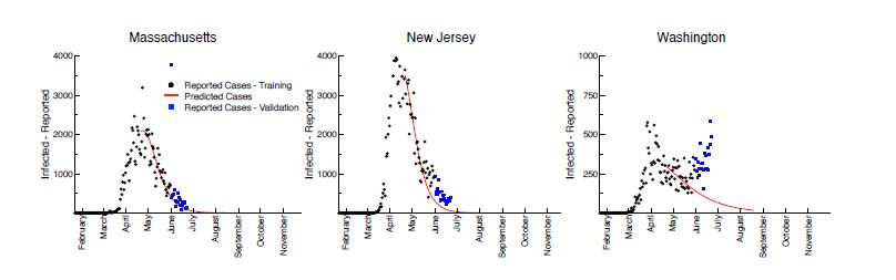
Page 6/12seen in our ts for Massachusetts, New Jersey, and Washington, in which the deterministic model was t
to time-series data from 22 January 2020 to 31 May 2020 (Figure 1). Here, black circles illustrate the new
daily reported infections, whereas the red curves illustrate the forecast associated with the median of the
ensemble trajectories identi ed through our Bayesian curve- tting method. Finally, the blue squares
illustrate the daily reported infec- tions since the model’s training, from 01 June 2020 to 22 June 2020.
Massachusetts and New Jersey have tracked well with the model’s predictions, while Washington has
seen a positive trend in new cases since the beginning of June not predicted by the model. This suggests
either a change in SIPOs policies in Washington, such as the introduction of the phased returns that
began 01 June 2020 [15], or changes in adherence and population behavior, resulting in out- breaks such
as those in agricultural businesses and long-term care facilities such as those seen in eastern
Washington [16], driving the increase. This highlights the primary limitation of the model: the resulting
forecasts are only applicable given a continuance of SIPOs policy and social behaviors.
Linking policy decisions to additional infection waves
Model ts to new daily case data are greatly improved if we sequester a fraction of sus- ceptible
individuals to limit access to infected ones (Fig. 1), but clearly these individuals do not inde nitely remain
immobile. If a goal of SIPOs is to minimize the extent and severity of COVID- 19 infections, then it seems
reasonable to lift them once infections fall below an acceptable level. What is this level and what
happens if SIPOs are removed too early or ignored, as we have seen in Washington and other states?
The Spanish Flu pandemic of 1918-1919 offers some insight, speci cally in that it pre- sented as three
successive waves of infections across the world [17, 18]. Mathematical modeling of this disease at a
population level suggests that its three infectious waves were rooted in the time dependence of its
population-averaged transmission rate [19]. Social factors, such as changes in population mobility, in
addition to others, can facilitate these trends. However, the Spanish Flu pandemic is thought to have been
affected by antigenic drift, which could also con- tribute changing immunity and transmission rates [20,
21]. A more general survey of mechanisms that might reproduce multiple infection waves for in uenza
pandemics suggests that a time-de- pendent transmission rate is su cient to t long-term infection
trends with low error [22]. This study also suggested that only very strong intervention (i.e., approx. 90%
reduction in initial sus- ceptibility) eliminated the appearance of second waves. Although the molecular
details of these viruses differ, these studies suggest that concepts such as a time-dependent
transmissibility and manipulation of susceptible populations are general enough to describe how
multiple waves of COVID-19 infections could evolve in the future.
We demonstrate a hypothetical second wave scenario for Massachusetts, New Jersey, and Washington in
Figure 2. A fraction of the population (70%, in this example) is reserved in isolation early in the simulation,
then released on 15 July 2020 when the SIPOs are relaxed in these scenarios. We then forecast through
the end of November for each state. States then see the peak of the second wave in mid-October to mid-
November 2020. Note that, without the re- implementation of social distancing, the second waves are
more severe than the rst, reaching over twice the number of active cases in the peak days compared to
Page 7/12the rst wave (Figure 2, black). We also test the scenario in which states stand up SIPOs starting 2 weeks
into the second wave, upheld through the end of the simulation. These policies result in a nearly-complete
atten- uation of the second wave (Figure 2, red). This result highlights the necessity to analyze current
policies and prepare populations to socially distance themselves as quickly as possible once an- other
wave is detected.
The effective reproductive number, Re, is a metric of the transmissibility of the virus; vi- ruses with Re
greater than 1 are likely to spread while those with R0 less than 1 are likely to die. An early review of Re
estimates for China found the average to be 3.28, with a median of 2.79 [23]. We have implemented a
“next-generation” matrix method to estimate the R0 for each day [11, 24]. This allows us to dynamically
track the Re and determine how changes in policy affect the transmissibility of the virus in state level
populations.
We demonstrate in Figure 3 the daily changes in the Re for the completely open and shel- tered-in-place
second wave scenarios for the three states. Initially, the Re ranges between 2-3.5 before dropping due to
changes in social distancing policy and behavior in the model. These then gradually decrease until Re is
less than 1. If current conditions are maintained, Re=1 quanti es a threshold below which the population
will eventually return to a disease-free state. Once the SIPO is lifted on 15 July 2020, the Re increases
back to approximately 1-2 due to an in ux of people from isolation, peaking in advance of secondary
infection waves. These Re values fall to below 1 again in the “open state” scenario, trending
monotonically down throughout the extent of the second wave. However, reimplementation of the SIPO 2
weeks after the second wave begins, sees Re values fall back below 1 where they persist, hearkening
back to the attenuation of the curve we demonstrated in Figure 2. This suggests that observation of a
dynamic Re could be used to monitor current and future waves of infections and to justify changes in
state policy and social behavior to mitigate public health impacts.
Conclusion
Ultimately, the ERDC SEIR represents a powerful tool to monitor the COVID-19 pandemic, as well as future
outbreaks of COVID-19 and other diseases by accounting for a range of drivers and stressors related to
population behavior and policy activity as well as daily-adjusted param- eters to calculate conditions that
may generate future waves of pandemic activity. In the near future, we anticipate making second wave
forecasts publicly available to further support USACE and FEMA responses and help guide state and
federal policy, while maintaining the production and distribution of forecasts. Finally, sudden events that
bring people together or induce mobil- ity, such as political protests and rallies or potential evacuations
resulting from hurricanes during the 2020 storm season have the potential to complicate our ability to
manage the COVID-19 pandemic, especially if people carry the virus into large congregations of people,
shelters or even other cities as well as emergency response teams being exposed. Overall, the ability to
under- stand the conditions and activities that fuel future waves can give policymakers and emergency
responders valuable time to prepare for and absorb COVID-19 disruptions, as well as consider actions
that may future mitigate disease spread.
Page 8/12Declarations
Opinions, interpretations, conclusions, and recommendations are those of the authors and are not
necessarily endorsed by the U.S. Army. The authors do not claim any con icts of interest.
References
1. S. Dong, H. R. Du, L. Gardner, An interactive web-based dashboard to track COVID-19 in real time.
Lancet Infect Dis 20, 533-534 (2020).
2. Patel, D. B. Jernigan, 2019-nCoV CDC Response Team, Initial public health response and interim
clinical guidance for the 2019 novel coronavirus outbreak - United States, December 31, 2019-
February 4, 2020 (Reprinted from Recomm Rep, vol 68, 2019). Am J Transplant 20, 889-895 (2020).
3. Pei, J. Shaman, Initial Simulation of SARS-CoV2 Spread and Intervention Effects in the Continental
US. medRxiv 2020.03.21.20040303, (2020).
4. IHME COVID-19 health service utilization forecasting team, Forecasting COVID-19 impact on hospital
bed-days, ICU-days, ventilator-days, and deaths by US State in th enext 4 months. medRxiv, (Murray,
CJL).
5. S. Army Corps of Engineers, Alternate Care Sites (ACS)
https://www.usace.army.mil/coronavirus/alternate-care-sites/. (2020).
6. W. Du et al., Risk for Transportation of Coronavirus Disease from Wuhan to Other Cities in China.
Emerg Infect Dis 26, 1049-1052 (2020).
7. Riou, C. L. Althaus, Pattern of early human-to-human transmission of Wuhan 2019 novel coronavirus
(2019-nCoV), December 2019 to January 2020. Eurosurveillance 25, 7-11 (2020).
8. Imai et al., Report 2: Estimating the potential total number of novel Coronavirus cases in Wuhan City,
China. https://www.imperial.ac.uk/mrc-global-infectious-disease- analysis/news--
wuhancoronavirus/, (2020).
9. M. Rong, L. Yang, H. D. Chu, M. Fan, Effect of delay in diagnosis on transmission of COVID-19. Math
Biosci Eng 17, 2725-2740 (2020).
10. Tahamtan, A. Ardebili, Real-time RT-PCR in COVID-19 detection: issues affecting the results. Expert
Rev Mol Diagn 20, 453-454 (2020).
11. Y. Li et al., Substantial undocumented infection facilitates the rapid dissemination of novel
coronavirus (SARS-CoV-2). Science 368, 489-+ (2020).
12. S. Center for Disease Control and Prevention (CDC).
(https://www.cdc.gov/coronavirus/2019-ncov/hcp/clinical-criteria.html, 2020).
13. Richardson, J. S. Hirsch, M. Narasimhan, Presenting Characteristics, Comorbidities, and Outcomes
Among 5700 Patients Hospitalized With COVID-19 in the New York City Area (Apr,
10.1001/jama.2020.6775, 2020). Jama-J Am Med Assoc 323, 2098-2098 (2020).
Page 9/1214. M. Dave, A. I. Friedson, K. Matsuzawa, J. J. Sabia, When Do Shelter-in-Place Orders Fight COVID-19
Best? Policy Heterogeneity Across States and Adoption Time. IZA Discussion Papers, No. 13190,
Institute of Labor Economics (IZA), Bonn, (2020).
15. King 5 Staff, Associated Press, in KING 5.
(https://www.king5.com/amp/article/news/health/coronavirus/washington-state- coronavirus-covid-
19-pandemic-updates/281-7e6196f3-0cf4-4dac-b2fa-999bbe334d73, 2020).
16. Blethen, in The Seattle Times. (2020).
17. K. Taubenberger, D. M. Morens, 1918 in uenza: the mother of all pandemics. Emerg Infect Dis 12, 15-
22 (2006)
18. Radusin, The Spanish Flu - Part II: the second and third wave. Vojnosanit Pregl 69, 917- 927 (2012).
19. H. He, J. Dushoff, T. Day, J. L. Ma, D. J. D. Earn, Mechanistic modelling of the three waves of the
1918 in uenza pandemic. Theor Ecol-Neth 4, 283-288 (2011).
20. K. Taubenberger, A. H. Reid, T. A. Janczewski, T. G. Fanning, Integrating historical, clinical and
molecular genetic data in order to explain the origin and virulence of the 1918 Spanish in uenza
virus. Philos T Roy Soc B 356, 1829-1839 (2001).
21. H. Reid, J. K. Taubenberger, T. G. Fanning, The 1918 Spanish in uenza: integrating history and
biology. Microbes Infect 3, 81-87 (2001).
22. Mummert, H. Weiss, L. P. Long, J. M. Amigo, X. F. Wan, A Perspective on Multiple Waves of In uenza
Pandemics. Plos One 8, (2013).
23. Liu, A. A. Gayle, A. Wilder-Smith, J. Rocklov, The reproductive number of COVID-19 is higher
compared to SARS coronavirus. J Travel Med 27, (2020).
24. M. Heffernan, R. J. Smith, L. M. Wahl, Perspectives on the basic reproductive ratio. J R Soc Interface
2, 281-293 (2005).
Figures
Page 10/12Figure 1
The ERDC SEIR model forecasts for Massachusetts, New Jersey, and Washington. The black dots
represent the number of active cases as represented by data, while the red line is the median number of
active cases predicted by the model.
Figure 2
The ERDC SEIR second wave hypothetical scenarios for Massachusetts, New Jersey, and Washington,
assuming a second wave start date of 15 July 2020. The black curves represent the median number of
reported infections predicted by the model if no social distancing policies are put in place to mitigate the
second wave. The red curves represent the median number of re- ported infections predicted by the model
if shelter-in-place policies are enacted 2 weeks into the wave.
Figure 3
The dynamic reproductive number for SARS-CoV-2 over the two wave scenarios for Massachusetts, New
Jersey, and Washington as presented in Figure 2. The black curves represent the reproductive numbers
over time for the open scenario, while the red curves represent the reproductive numbers over time for the
shelter-in-place scenarios.
Page 11/12Supplementary Files
This is a list of supplementary les associated with this preprint. Click to download.
ERDCSEIRSI.pdf
Page 12/12You can also read