Modifiable Areal Unit Problem (MAUP): Analysis of Agriculture of the State of Paraná-Brazil - Agris on-line Papers ...
←
→
Page content transcription
If your browser does not render page correctly, please read the page content below
Agris on-line Papers in Economics and Informatics
Volume XIII                                                                                       Number 2, 2021

Modifiable Areal Unit Problem (MAUP): Analysis of Agriculture
of the State of Paraná-Brazil
Elizabeth Giron Cima1, Weimar Freire da Rocha-Junior1, Miguel Angel Uribe-Opazo1, Gustavo Henrique
Dalposso2

1
    Western Paraná State University (UNIOESTE), Cascavel-PR, Brazil
2
    Federal University of Technology – Paraná (UTFPR), Toledo-PR, Brazil

Abstract
The way the researcher groups his research data will influence the result of his work. In the literature, this
phenomenon is treated as a Problem of the Modifiable Areal Unit. The objective of this article was to analyze
the three spatial levels by Municipalities, Regional Centers and Mesoregions using the following data:
gross domestic product, effective agricultural production, grain production and gross value of agricultural
production for the state of Paraná-Brazil in the period since 2012 until 2015. The methodological procedure
studied data from the Paranaense Institute for Economic and Social Development of the above-named
variables collected on the website of the Paranaense Institute for Economic and Social Development
of the 399 municipalities, 23 regional centers and 10 mesoregions. The results found show the presence
of the Modifiable Areal Unit Problem, presenting different results for each level of grouping. The study
revealed the problem of the modifiable areal unit is a relevant occurrence and it should be disregarded
by researchers who work with clusters of spatial data in their studies. The results found allow a better
understanding of the scale effect and demonstrate the efficiency of spatial analysis in socioeconomic data.

Keywords
Aggregation, agribusiness, autocorrelation, scale effect, spatial process, decision making

Cima, E. G., Freire da Rocha-Jr., W., Uribe-Opazo, M. A. and Dalposso, G. H. (2021) "Modifiable Areal
Unit Problem (MAUP): Analysis of Agricultural of the State of Paraná-Brazil", AGRIS on-line Papers
in Economics and Informatics, Vol. 13, No. 2, pp. 35-50. ISSN 1804-1930. DOI 10.7160/aol.2021.130203.

Introduction                                                    obtained within a system of area units are directly
                                                                related to different ways in which they can be
Following the development of science, new                       grouped and consequently different results can be
challenges are imposed on researchers, once new                 obtained by simply alteration of the boundaries
problems arise, consequently, new resolutions are               established (Janelle et al., 2004; Wei et al., 2017;
proposed, according to Kupriyanova et al. (2019).               Duque et al., 2018; Didier and Louvet, 2019).
Surveys work with different spatial boundaries
for the analysis of the most varied themes, in which            Some studies, already carried out, realized
the relationship between time and space is analyzed,            the importance of MAUP in spatial data (Lee et al.,
the size of the clusters changes and the phenomenon             2015; Cabrera-Barona et al., 2018; Pietrzak, 2019).
entitled Modifiable Areal Unit Problem (MAUP)                   Investigating the effect of MAUP aims to study
can present different results according to the spatial          various sizes of spatial resolutions that can lead
boundaries are changed. Observation and evaluation              researchers to determine the most appropriate scale
of the effects of the Modifiable Areal Unit Problem             to be used for analysis purposes, Wei et al. (2017)
become a relevant issue in the modeling, because                report that the effects of MAUP can be completed
if the appropriate levels of geographic scale                   through statistical results.
and zone configuration are not defined                          Chaves et al. (2018) report that the problem
and identified; statistical models based on spatial             modifiable areal unit can alter the support
data can induce the misleading conclusions.                     of soybean cultivation, inform that is not possible
Thus, considering the same population under                     to cultivate soybean and other crops in the same
study, the spatial definition of its borders affects            environment simultaneously, highlight that MAUP
the results will be obtained. The estimations                   is related to two specific problems, namely:

                                                         [35]
Modifiable Areal Unit Problem (MAUP): Analysis of Agricultural of the State of Paraná-Brazil
the scale effect and zoning effect, economically this the regression coefficients at the local level.
result may compromise the planning of soybean The spatial regression methods allow taking into
productivity. account the dependence between the sample elements
collected in regions considering the location
Lee et al. (2018) in their studies found that
of the data (Lesage, 2015; Duan et al., 2015).
the problem of the modifiable areal unit has
a clear and evident scale effect for the uncertainties This article presents a study of MAUP
surrounding its relations with spatial autocorrelation, from a database of the gross domestic product,
identified in their experiments with simulation, that effective of agricultural production, total grain
in an initial level, autocorrelation spatial plays production and gross value of agricultural
an important role in the nature and extent production, obtained through the Paranaense
of the effects of MAUP. Institute of Economic and Social Development
(IPARDES) in the years 2012 to 2015. The analysis
According to the United Nations Program
focused on three levels: Municipalities, Regional
for Sustainable Development - UNDP (2020)
Centers and Mesoregions. The objective of this
suggest that researchers should work with
study was to analyze the MAUP, in the state
disaggregated data in economic analyzes according
of Paraná-Brazil, using different spatial resolutions
to the 2030 Agenda that addresses the Sustainable
and to show the extent to which the different scale
Development Goals (SDGs).
effects can directly reflect in the decision making
Salmivaara (2015), Santo et al. (2015), Cabrera- of regional analyzes of public and private
Barona et al. (2016) and Burdziej (2019) studied institutions in the agribusiness economics.
and evaluated the scale effect (MAUP) at different
levels of spatial units. Recent studies consider Materials and methods
the scale effect in decision-making (Xu et al., 2018;
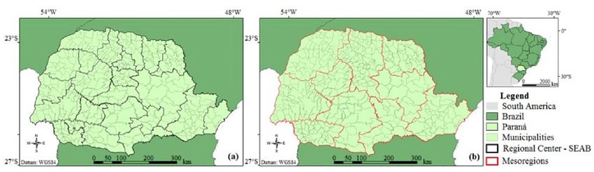
Tunson et al., 2019). The study area comprises 399 municipalities,
23 regional development centers (Figure 1a)
Anselin (2018) presents Geary's global univariate
and 10 mesoregions (Figure 1b) in the state
index (c) and Geary's local (ci) to study the spatial
of Paraná. Socioeconomic data from the years 2012
autocorrelation of quantitative characteristics
to 2015 and the variables were used: gross domestic
considering the location of the data. Spatial
product [R$], effective agricultural production
regression models, such as spatial autoregressive
[quantity/unit], gross value of agricultural
(SAR), conditional autoregressive (CAR)
production [R$], Total grain production (soybeans,
and geographically weighted spatial model
corn 1st harvest, corn 2nd harvests, and wheat) [t].
(GWR), are established to study the relationship
of an interested variable to its covariables and For the analysis of spatial autocorrelation,
considering the location of the data and from your the hypothesis test was used by means of the Z(c)
close neighbors. (Anselin and Bel, 2013; Araújo pseudo-significance statistic (Almeida, 2012).
et al., 2014; Meyappan et al., 2014; Javi et al.,
Exploratory Spatial Data Analysis was applied
2015; Zou and Wu, 2017). The SAR and CAR
to this database to identify its global spatial
models are considered global models; their
associations and clusters. Then, the spatial
results are valid for the entire study area, whereas
regression models SAR, CAR and GWR were
the GWR explores local variations and estimates
Source: Adapted from SEAB-DERAL (2015)
Figure 1: Delimitation of study area (Figure 1a and Figure 1b).
[36]
Modifiable Areal Unit Problem (MAUP): Analysis of Agricultural of the State of Paraná-Brazil

applied to verify which model best explains                      significant spatial clusters, and the property that
the gross value of agricultural production (Vpb).                the sum of ci for all regions is proportional
For the analysis of spatial autocorrelation, the                 to the indicator of global spatial autocorrelation
global Geary index (c) (Equation 1) was used, which              c by Geary (Anselin, 2018).
allows the assessment of global autocorrelation.
                                                                                                                (3)
The Geary global index (c) assumes the spatial
autocorrelation depends on the distance between                  The linear spatial models SAR, CAR and GWR
two or more observations, assumes the values                     estimated by maximum likelihood for gross value
between 0 and 2 (ANSELIN, 2018), and if c = 0,                   of agricultural production (Vpb) as a function
it indicates direct positive spatial autocorrelation;            of the total quantity of bovine production
if c = 1, it indicates absence of autocorrelation and            (QTbovine), total quantity of pig production
if c > 1, it indicates negative spatial autocorrelation          (QTpig), total quantity of production of poultry
(Anselin, 2018).                                                 (QTpoultry) and total amount of grain production
                                                                 (Totgrain) are presented in Equations (4), (5)
                                                   (1)           and (6), respectively:

on what,
n: number of spatial units (areas);                                                                             (4)
xi and xj: values of attribute X considered in regions
i and j;
  : average value of attribute X in the studied region;                                                         (5)

wij: element of the normalized neighborhood
matrix, corresponding to the spatial weights 0
and 1, being 0 for areas i and j that do not border
between themselves and 1 for areas i and j that                                                                 (6)
border between each other. In this work, the Queen
Contiguity criteria (Anselin, 2018) was used.                          estimated parameters of each model (SAR,
                                                                 CAR and GWR), y = 0,…, 4;
Considering the following hypothesis test
                                                                 WVpb: expresses the weighted spatial dependence
H0: There is no association between the observed
                                                                 with weight allocation of the spatial neighborhood;
value in a region and the observed value in nearby
regions, c values are close to 1; versus                             estimated autoregressive spatial coefficient;
H1: There is an association between nearby                            estimated autoregressive coefficient;
regions, c values are close to 0. In order to verify             Wɛ: error component with spatial effects,
the significance of the global Geary index (c),
                                                                 (ui, vi): denotes the coordinates of the centroid
if there is no association between the value observed
                                                                 of the i-th area, i = 1, ..., 399;
in a region and the value observed in nearby regions,
it is done through the pseudo-significance statistic                                  realization of the continuous
Z (c) (Equation 2) (Anselin, 2018).                              function          on the ketoid of the i-th area,
                                                                 i = 1,…, 399 (Fotheringhan et al., 2002).
                                                   (2)           Lopes et al. (2014) employed, in the comparison
                                                                 of the SAR, CAR and GWR models, the highest
where, E(c) is the expected value of the Geary
                                                                 value of maximum likelihood logarithm (MLL),
global index (c); Sd(c) is the standard deviation
                                                                 which represents the best fit to the observed data.
of Geary's global index (c). About H0, the Z(c)
                                                                 The Akaike Information Criterion (AIC)
statistic has a standard normal distribution
                                                                 and the Baysian Criterion (BIC) were also used
with mean 0 and variance 1 (Almeida, 2012).
                                                                 in this study, considering the best model is which
Geary's     local  autocorrelation   index    (ci)               has the lowest value of AIC and BIC (SPRING,
(Equation 3), which measures the degree of spatial               2003).
correlation at each specific location (Anselin,
                                                                 The data analysis was performed with the aid
2018). The local statistic ci is an indicator
                                                                 of free software R (R Core Team, 2018).
of spatial association called LISA because it
                                                                 The following packages were used: GISTools,
satisfies two requirements, namely: the ability
                                                                 Spdep, Spgwr, Rgeos and Nortest.
for each observation to signal statistically

                                                          [37]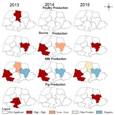
Modifiable Areal Unit Problem (MAUP): Analysis of Agricultural of the State of Paraná-Brazil

Results and discussion                                                      productive and economic potential.

On Table 1, they are presented Geary global spatial                         With this information, it is possible to develop public
autocorrelation indexes (c) and Z(c) significance                           policies in municipalities with disparate results
tests, for Gross Domestic Product (GDP), bovine                             and in municipalities with low productivity detect
production, Pig production, Poultry production,                             problems and improve production. The information
Production of milk, Gross value of agricultural                             can thus subsidize state agricultural policies
production, Grain production for the municipalities                         in the municipalities with the greatest difficulties,
belong to Paraná state (Brazil).                                            in the case of milk there is a very high contingent
                                                                            of family farmers.The global Geary index (c)
It is possible to check in the 2012’s GDP,                                  for each year studied by the Regional Centers
Geary's global spatial autocorrelation index was                            (Table 2) indicated positive spatial autocorrelation
not significant, realized the absence of spatial                            of 5% significance for the production of bovine,
autocorrelation.This result is justified according                          pig and poultry, and gross value of agricultural
as inform IBGE (2012) this period there were                                production.
climatic problems such as the drought in the first
half, affecting crops and the retraction of factory                         However, in the product gross domestic product
production in the state of Paraná-Brazil. For 2013,                         and in the total production of grains (soybeans,
2014 and 2015, there are some significant positive                          corn 1st and 2nd harvest and wheat) there were
spatial autocorrelation of the GDP.                                         no significant spatial autocorrelation because
                                                                            the indices were close to one, presenting the data
There was a significant positive spatial                                    are randomly distributed over the analyzed years.
autocorrelation for all variables studied. This
behavior shows that in the Paraná state, there are                          From this point, the presence of the problem
municipalities with high and /or low livestock                              of the modifiable areal unit (MAUP) begins to be
production, total grain production and gross                                perceived in which by changing the spatial level
value of agricultural production surrounded                                 of area, different statistical results are obtained
by municipalities that have similar characteristics,                        (Table 2). Jiawei et al., (2020) comment that
with the mean spatial autocorrelation being                                 the spatial scale is also a major concern
c̅ = 0.5016. (Table 1).                                                     in the research on grain production and so, as you
                                                                            highlight Chen (2018),when choosing analytical
Economically it is observed through the results                             units to quantify regional economic structure
found, specifically for the production of milk                              for a specific study, future research should pay
and production of poultry, values close to zero,                            attention to scale-related problems.
which implies that municipalities economically with
high and or low production of these commodities                             Comparing the spatial level of the regional centers
are surrounded by neighbors also with high and                              and the spatial level of the municipalities, through
or low productions, this information is economically                        Geary's global analysis (c) the results show
very necessary and important because it allows                              the presence of a MAUP effect in the Gross
showing the reality of the economic and agricultural                        Domestic Product and in the Total grain production,
scenario of these locations, thus highlighting their                        as it is possible to check in the Tables (1) and (2).

    Variables                                           2012                    2013                   2014                    2015
    GDP                                                0.928Ns                 0.794*                 0.790*                  0.827*
    Bovine production                                  0.525*                  0.522*                 0.510*                  0.509*
    Pig production                                     0.421*                  0.421*                 0.402*                  0.412*
    Poultry production                                 0.590*                  0.592*                 0.629*                  0.613*
    Milk Production                                    0.397*                  0.395*                 0.369*                  0.361*
    Gross value of agricultural production                 .                   0.668*                 0.621*                  0.674*
    Grain production                                   0.408*                  0.410*                 0.403*                  0.456*

   Note: Ns - not significant values; * statistically significant at the level of 5% probability; . - absence of information in the official
   database.
   Source: own calculations
     Table 1: Global Geary Index (c) of gross domestic product (GDP), actual agricultural production (bovine, pig, poultry, milk),
      gross value of agricultural production and total grain production (soybeans, corn 1st and 2nd harvest) and wheat) since 2012
                            until 2015 of the three hundred and ninety-nine municipalities in Paraná-Brazil.

                                                                    [38]
Modifiable Areal Unit Problem (MAUP): Analysis of Agricultural of the State of Paraná-Brazil
Variables 2012 2013 2014 2015
GDP 0.900Ns 0.920Ns 0.895Ns 0.954Ns
Bovine production 0.514* 0.515* 0.541* 0.536*
Pig production 0.557* 0.557* 0.560* 0.572*
Poultry production 0.610* 0.611* 0.561* 0.548*
Milk Production 0.418* 0.415* 0.405* 0.391*
Gross value of agricultural production . 0.751* 0.683* 0.701*
Grain production 0.850 Ns
0.868 Ns
0.900 Ns
0.861Ns
Note: Ns - not significant values; * statistically significant at the level of 5% probability; . - absence of information in the official
database.
Source: own calculations
Table 2: Global Geary Index (c) of gross domestic product (GDP), effective agricultural production (bovine, pig, poultry, milk),
gross value of agricultural production and total grain production (soybeans, corn 1st and 2nd harvest) and wheat) from the years
2012 to 2015 of the twenty-three regional centers of SEAB-Paraná-Brazil.
Therefore, it shows the problem of the modifiable The Modified Areal Unit Problem in the three
areal unit can reflect negatively on the decision- verified spatial levels had a relevant presence,
making process of public and private agencies mainly in the regional centers and mesoregions
(Table 2). when compared to municipalities, evidences
of it were the values analyzed in the mesoregions
In the Table 3, the global index of Geary (c)
where were not significant for any variable studied
by Mesoregions belonging to Paraná state
(Table 3).
demonstrates the presence of MAUP, because
all indexes c presented values close to 1, a value These results showed the importance of the MAUP
indicative of a random spatial pattern, a fact study in the decision-making process and it
corroborated by the test of pseudo-significance suggests how necessary is consider the possibility
Z(c), which indicates absence of significant spatial of individual differences between the analyzed
autocorrelation. variables and the individual difference cannot be
generalized, which is corroborated by Burdziej
In the analysis of Geary's global autocorrelation
(2019).
(c) for the Mesoregions of Paraná, Table (3) shows
a high effect of the Modified Areal Unit Problem Geary's local autocorrelation indexes (ci) are
(MAUP) in all studied variables, it means that presented using the LISA Cluster Map for poultry
the statistical results found were quite different production from 2013 to 2015 by municipality,
from those found in municipalities and regional in Figure 2. The result shows spatial grouping
centers. All values of the Geary index (c) which of points in the studied regions, namely: West,
were close to 1 characterized absence of spatial Southwest, Central South and part of the North
autocorrelation. Central region, suggesting significant positive
spatial autocorrelation, having regions with high
This spatial behavior shows how serious
or low production of birds surrounded by regions
the Modifiable Area Unit Problem (size
with similar characteristics (dark red color and pink
of the spatial resolution) is, considering the same
color in Figure 2).
study population. Comparing the three studied
spatial levels (municipalities, regional centers and It was also observed the presence of negative
mesoregions) (Table 1, Table 2 and Table 3), it is spatial autocorrelation during 2013, 2014
required the decision-making process must respect and 2015; it suggests regions with high and/or
to the different results found and the decision should low poultry production surrounded by neighbors
be made cautiously, in the sense order to better with similar characteristics and regions with low
understand the different results of the spatial levels poultry production, surrounded by regions
analyzed associated with the real study scenario. with high poultry production, in the light blue color
Considering the same population of studies, of Figure 2.
the different scales tested must be consistently
It is observed the Modifiable Areal Unit Problem
evaluated, begin that many studies point
(MAUP) is very visible when comparing
to the use of disaggregated data. It is suggested
the Municipal Map (Figure 2) to the Regional
non-generalization of the facts, it means, they all
Centers Map (Figure3), there is a significant
share a similar characteristic.
[39]Modifiable Areal Unit Problem (MAUP): Analysis of Agricultural of the State of Paraná-Brazil
Variables 2012 2013 2014 2015
GDP 1.160 Ns
1.159 Ns
1.128 Ns
1.211Ns
Bovine production 0.943 Ns
0.943 Ns 1.002 Ns
0.995Ns
Pig production 0.959Ns 0.959 Ns 0.977Ns 1.028Ns
Poultry production 0.759 Ns
0.759 Ns 0.794Ns 0.802Ns
Milk Production 0.702Ns 0.702Ns 0.755 Ns 0.759Ns
Gross value of agricultural production . 1.234 Ns 1.181 Ns 1.216Ns
Grain production 1.142 Ns
1.151 Ns
1.165 Ns
1.118Ns
Note: Ns - not significant values; * statistically significant at the level of 5% probability; . - absence of information in the official
database.
Source: own calculations
Table 3: Global Geary Index (c) of gross domestic product (GDP), effective agricultural production (bovine, pig, poultry, milk),
gross value of agricultural production and total grain production (soybeans, corn 1st and 2nd harvest) and wheat) from the years
2012 to 2015 of the twenty-three regional centers of SEAB-Paraná-Brazil.
Source: own research
Figure 2: LISA Cluster Map maps, related to poultry production, bovine, milk and pig by municipalities for the years 2013 to 2015.
difference between them. This results corroborates Through Geary's local autocorrelation index (ci),
with the results obtained by Zen et al., (2019), who it is observed, in the bovine production from 2013
accessed the sensitivity to the MAUP, by calculating to 2015 (Figure 2), spatial patterns of clusters
global statistics over there grid displacements. occur. In which, it is present positive spatial
[40]Modifiable Areal Unit Problem (MAUP): Analysis of Agricultural of the State of Paraná-Brazil
autocorrelation and negative spatial autocorrelation, of the municipalities, there was a greater frequency
it means, the producing regions are similar to each of significant positive spatial autocorrelation,
other and they are close to each other, as well represented by the colors dark red and pink
as regions distant from each other, allowing in Figure 2, with a predominance of regions with
the identification of significant clusters (5%) shown high milk production, surrounded by neighbors
in Figure 2, light pink. also with high milk production, mainly in the West,
Southwest and Center South regions.
In the 399 municipalities of Paraná state, it was
observed clusters of municipalities with high Regions with significant negative spatial
bovine production surrounded by neighbors autocorrelation were also observed, mainly
with similar characteristics (dark red color in the Metropolitan Region and Eastern Center,
in Figure 2). The pattern of spatial concentration in Figure 2, identified as light blue color.
was observed most frequently in the municipalities The results demonstrate the pig production,
of Guarapuava, Pitanga, Laranjeira do Sul, for the years studied presented, in its great majority,
Catanduvas, Boa Vista de Aparecida, Guaraniaçu positive spatial autocorrelation (Figure 2, in dark red
and Umuarama. Municipalities with significant and pink colors), emphasizing on the mesoregions,
negative spatial autocorrelation were observed, namely, Centro Oriental, North Central, South
it means, municipalities with high bovine Center, West and Northwest.
production surrounded by municipalities
It is important to note, for the year 2013, there were
with low bovine production (light blue color
municipalities with high pig production surrounded
in Figure 2) and municipalities with low cattle
by neighbors with this same characteristic,
production surrounded by neighbors with high
in the West, Center South and part of the
bovine production, this behavior signals spatial
Central Eastern region, for 2014 and 2015,
outliers, showing low spatial interaction between
these same similarities were observed in parts
the municipalities.
in the municipalities belonging to the Northwest
Between 2014 and 2015, it was observed that and North Pioneiro regions. In 2014 and
there was a greater spatial concentration of data 2015, there was a decrease in pig production
showing similar characteristics (High-High) in the municipalities (Low-Low) represented
in the municipalities of Guarapuava, Laranjeira in pink. This fact may be related to the high
do Sul, Loanda, Altonia, Três Barras, Catanduvas, production costs of this herd, which corroborates
Campo Bonito, Umuarama, Altamira do Paraná Embrapa, (2016) who studied the costs of pig
and Quedas do Iguaçu. This behavior may be related production in the main states of Brazil, including
to the incentive in the use of confinement technique, Paraná and as a result, he found the variable
which allows greater control over production costs. most influencing the costs of pig production is
the cost of labor, this result is relevant, since
The adoption of the bovine confinement system
agricultural production also fluctuates according
allows greater gains in production and signals
to the prices practiced in the markets associated
that it is a profitable and viable livestock activity
with the production costs borne by rural producers,
(Barbieri; Carvalho and Sabbag, 2016). This
if the price to be paid to the finished final product is
technique allows to concentrate more animals
not attractive, the tendency is that much producers
per area and consequently to have a larger scale
choose to migrate to other more profitable activities.
reducing costs, besides obtaining bigger gains
when providing more concentrated food without Considering that livestock production is
generating the movement of the animal generating economically demanding, a viable alternative
greater added value to the product at the time would be to add technologies, investments in labor
of commercialization, allowing greater gains (technical and professional education) in order
to the producers. to improve good agricultural practices by promoting
greater incentives to the activity that requires a lot
Regions that are not prone to agricultural
of experience and planning on the part of rural
cultivation due to steep topographic conditions,
producers.
relief demographics, among others, which do not
favor the planting of agricultural crops, are destined The results presented in Figure 3, for poultry
for other activities such as bovine raising. production, point out three significant clusters
Cultivation techniques, no-till techniques are (High-High) just for the regional centers
restricted in these environments. of Cascavel, which differentiates it in great
relevance to the map of the municipalities (Figure
Considering milk production, in most
[41]Modifiable Areal Unit Problem (MAUP): Analysis of Agricultural of the State of Paraná-Brazil
2 in the dark red shade). This difference is Centers and Mesoregions are quite different
accentuated when compared to the results from those observed in the municipal map
of the mesoregions, as shown in Figure 4, (Figure 3 and Figure 4). The significant cluster
for the year 2013, which characterizes the MAUP, agglomeration suggesting positive spatial
in which there was a high-high cluster just autocorrelation for bovine production appears
for the North Central mesoregion, already in the regional centers of Pitanga, Laranjeira
for the years 2014 and 2015 there were no clusters do Sul, Francisco Beltrão, Paranavaí, Maringá
with significant results. The statistical results are and Cianorte (Figure 3 in brown). The regional
different. There was the presence of a Low-Low centers that make up the municipalities of the West
group, mainly in the Regional Centers of Pitanga, region practically disappear in 2013 and 2014
Guarapuava, Irati and União da Vitória (Figure 3 (Figure 3 in white).
in pink).
The same fact occurs in the mesoregions
The MAUP is clearly observed, comparing (Figure 4). On the other hand, in 2015, the regional
the maps made from the same database, the results center of Cascavel, Toledo, Guarapuava and União
of the significant clusters of the Regional da Vitoria presented a cluster (Low-Low), and their
Source: own research
Figure 3: LISA Cluster Map maps, relative to the production of poultry, bovine, milk and pig by Regional Centers for the years
2013 to 2015.
[42]Modifiable Areal Unit Problem (MAUP): Analysis of Agricultural of the State of Paraná-Brazil
municipalities were not identified on the municipal Therefore, as it appears in the municipal data, it
map, suggesting the difference between these is necessary to have coherence and consideration
maps. For milk production, the result also shows when analyzing the data by regional centers.
the presence of MAUP, demonstrating significant The MAUP is clearly visible in these presented
differences between maps of municipalities results. The group considering different spatial
and maps of regional centers, Roces-Díaz et al. resolutions can generate complications in decision-
(2018) comment that when analyzing spatial data making process, which in fact shows it in this
in different scales, they found different results analysis. For the production of pigs in 2013,
between the levels studied, concluded that the use significant clusters (High-High) were observed
of spatial data in different resolutions, the results in the following regional centers: Toledo, Cascavel,
found showed significant differences. Dois Vizinhos, Laranjeira and Guarapuava
(Figure 3 in dark red). In 2014 and 2015, there
The result points to significant clusters, suggesting
were significant regional clusters in these same
positive spatial autocorrelation (High-High) just
regions (Low-Low), which is very different
for the regional centers of: Cascavel, Laranjeira
from the municipal map and map by mesoregion
do Sul, Francisco Beltrão, Dois Vizinhos, Pato
(Figure 3), once other regions had this characteristic.
Branco, Irati and Umuarama. Toledo regional
center (major producer milk from Western Paraná) The results found make sense, because there was
simply disappeared from the map (Figure 3). a slowdown in pig production in 2014 and 2015 due
Source: own research
Figure 4: LISA Cluster Map maps, relative to the production of poultry, bovine, milk and pig by Mesoregions for the years
2013 to 2015.
[43]Modifiable Areal Unit Problem (MAUP): Analysis of Agricultural of the State of Paraná-Brazil
to the high production costs (EMBRAPA, 2016). function - 160.670. The other indexes point
It was observed constant productions in these to a model adjusted with the addition of spatial
periods. The results presented in Figure 4 dependence on the response variable
demonstrate the MAUP to the production of poultry, = 0.45283. The results inherent to the application
bovine, milk and pig. Comparing the maps made of the CAR model to estimate the gross value
through the three levels of differentiated spatial of agricultural production (Vpb) to 2013 explains
resolutions, the results of the significant clusters R2 = 77.8%, presenting a significant autoregressive
of the Mesoregions are different from those coefficient λ (Lambda) (0.490*), showing that
observed in the maps of the Municipalities and spatial autocorrelation attributed to the error was
maps of the Regional Centers (Figure 4). significant at the 5% level of significance (Table 4).
The municipality agglomeration in the West Table 4 also shows the estimated GWR model
Mesoregion practically disappeared to the effective for the gross value of agricultural production (Vpb)
production of poultry and pig production in 2014 with a determination coefficient R2 = 83.3%.
and 2015 in the state of Paraná (Figure 4), which It shows that there was, through the analysis
suggests how worrying the problems were, which of the GWR model, the best fit, considering
can occur mistaken decision-making process, the SAR and CAR models, once it presented
when analyzed through the same study population the highest MLL value and the lowest values
considering a single level of analyzed spatial for AIC and BIC. Therefore, the local GWR
resolution. model was the best explanation to the gross value
of agricultural production (Vpb) for the year 2013.
For each year (2013, 2014 and 2015), SAR, CAR
and GWR models of the gross value of agricultural Table 5 shows the results of the SAR, CAR
production (Vpb) were built in relation to livestock and GWR models of the gross value of agricultural
production and total grain production for each year, production (Vpb) in 2014 for the municipalities.
considering the existence of spatial autocorrelation. In all models, the estimated parameter 2
is
The results to the municipalities in the state negative, which implies an inversely proportional
of Paraná are presented in Tables 4, 5 and 6. effect of the total quantity of pigs (QTpig)
in the gross value of agricultural production (Vpb)
The SAR, CAR and GWR forecast models
for the year 2014, in the years 2014 to 2015 there
for the gross value of agricultural production (Vpb)
was retraction in the production of pig, which
considering the explanatory variables: total amount
may be related to the high production costs in this
of bovine production (QTbovine), total amount
activity (IBGE, 2016).
of pig production (QTpig), total amount of poultry
production (QTpoultry) and total amount of grain The results also showed, for 2014, the best model,
production (Totgrain) for the year 2013, are shown which explains the estimate of the gross value
in Table 4. of agricultural production (Vpb), was the GWR
model. As it is a local model, it attributed
All the estimated parameters ´s are observed
a significant improvement to the spatial regression
in all models are positive, which implies a directly
process in the studied region (Table 5).
proportional influence of the herds of the livestock
production and total grain production in 2013. In 2015, it was observed, similarly to previous
years, the GWR model was the best explanation
The result indicated the response variable: the SAR
to the gross value of agricultural production (Vpb)
autoregressive model at R2 = 77.32% explained
as a function of cattle production, pig production,
gross value of agricultural production (Vpb)
poultry production and total grain production
in 2013 (coefficient of determination).
of the 399 municipalities of Paraná (Table 6).
The Maximum logarithm value of the likelihood
Statistics MLL R2 AIC BIC
0 1 2 3 4
SAR 2.734 0.043 0.081 0.452 0.076 0.452* - - 160.670 0.774 343.340 387.163
CAR 4.32 0.053 0.080 0.451 0.074 - 0.490* - 165.013 0.778 344.026 371.913
GWR 4.55 0.042 0.093 0.430 0.067 - - 0.310 0.833 322.957 311.735
Note: * significant probability level of 5 %; , auto-regressive coefficients; MLL: maximum likelihood logarithm ratio; R2 adjusted
coefficient of determination; AIC: Akaike information criterion; BIC: Bayesian information criterion; bold: best adjusted model.
Source: own calculations
Table 4: Statistical results of the SAR, CAR and GWR models for the gross value of agricultural production in 2013 for municipalities.
[44]Modifiable Areal Unit Problem (MAUP): Analysis of Agricultural of the State of Paraná-Brazil
Statistics MLL R2 AIC BIC
0 1 2 3 4
SAR 10.970 0.0097 -2.461 0.287 0.065 0.451* - -195.165 0.773 412.329 456.153
CAR 17.259 0.0901 -2.825 0.283 0.064 - 0.492* -199.548 0.768 413.095 440.983
GWR 18.109 0.073 -3.580 0.262 0.057 - - 0.340 0.831 354.374 343.152
Note: * significant probability level of 5 %; , auto-regressive coefficients; MLL: maximum likelihood logarithm ratio; R2 adjusted
coefficient of determination; AIC: Akaike information criterion; BIC: Bayesian information criterion; bold: best adjusted model.
Source: own calculations
Table 5: Statistical results of the SAR, CAR and GWR model for the gross value of agricultural production in 2014 for municipalities.
Statistics MLL R2 AIC BIC
0 1 2 3 4
SAR 6.627 0.138 -2.369 0.381 0.062 0.400* - -243.147 0.793 508.295 552.118
CAR 7.710 0.118 -2.862 0.373 0.064 - 0.469* -252.732 0.783 519.464 547.351
GWR 7.744 0.025 0.341 -0.036 0.089 - - 0.393 0.840 400.421 393.021
Note: * significant probability level of 5 %; , auto-regressive coefficients; MLL: maximum likelihood logarithm ratio; R2 adjusted
coefficient of determination; AIC: Akaike information criterion; BIC: Bayesian information criterion; bold: best adjusted model.
Source: own calculations
Table 6: Statistical results of the SAR, CAR and GWR model for the gross value of agricultural production in 2015 for municipalities.
In similar way of studies based on municipal the GWR model, it was possible to adjust a model
database, the SAR, CAR and GWR models for the gross value of agricultural production
to Regional Centers of the state of Paraná-Brazil (Vpb) for the studied years, this fact is justified
were studied. because the estimation of the parameters takes into
account the spatial information, Table 10, Table 11
It is observed according to the results presented
and Table 12.
in Tables 7 to 9 that the parameters ,
of the SAR and CAR models are not significant. In accordance with Table 11 and Table 12, it was
The geographically weighted spatial regression observed the SAR and CAR models were also
model (GWR) was the best representation not significant, showing the spatial structure is
of the gross value of agricultural production (Vpb) not being incorporated into the model, which
in the three years 2013 to 2015. Therefore, resulted in a multivariate regression model,
the result shows the SAR and CAR models with a significant degree of explanation
of the gross value of agricultural production for the studied variables. Indeed, this fact confirms
(Vpb) is associated to the study unit that are the scale effect, characterizing the presence
the municipalities. of MAUP in the studied mesoregions.
Whereas just in the regional centers Therefore, the MAUP is visible in the study,
and mesoregions, the GWR model is significantly considering the comparative analysis of the SAR,
related to production of bovine, pigs, poultry CAR and GWR models. The GWR model was
and grains. In this sense, the MAUP effect is the one that explained the variable response gross
observed in the database of regional centers value of agricultural production.
and mesoregions. This result corroborates
In the analysis of these models, it was clear
the results obtained by Jonatan and Brewer (2017),
the presence of MAUP in the comparison among
who, in their findings, verified that the aggregated
the results based upon municipal, regional center
data are sensitive to MAUP, and the levels
and mesoregions databases.
of aggregation, sizes and zones, affect the validity
and reliability of the results. Their findings suggest
that researchers need to choose the most appropriate
scale for specific problems analyzes.
It is evident the presence of MAUP (Table 7,
Table 8 and Table 9) in the analysis of the spatial
level by regional centers. MAUP is also observed
in the mesoregions for the models (SAR and CAR),
once the parameters related to the spatial level were
not significant in any studied year. Considering
[45]Modifiable Areal Unit Problem (MAUP): Analysis of Agricultural of the State of Paraná-Brazil
Statistics MLL R2 AIC BIC
0 1 2 3 4
SAR 11.150 -0.039 0.393 0.137 -0.045 -0.341 Ns
- 2.797 0.829 16.405 28.895
CAR 5.450 -0.022 0.316 0.313 -0.021 - 0.030Ns 0.181 0.785 13.636 21.584
GWR 5.485 -0.022 0.316 0.310 -0.022 - - 0.234 0.795 24.392 13.170
Note: * significant probability level of 5 %; , auto-regressive coefficients; MLL: maximum likelihood logarithm ratio; R adjusted
2
coefficient of determination; AIC: Akaike information criterion; BIC: Bayesian information criterion; bold: best adjusted model.
Source: own calculations
Table 7: Statistical results of the SAR, CAR and GWR model of the gross value of agricultural production by regional centers in 2013.
Statistics MLL R2 AIC BIC
0 1 2 3 4
SAR 37.323 -0.042 -11.486 0.033 -0.040 -0.537Ns - 7.605 0.90 6.788 19.278
CAR 25.106 -0.013 -9.817 0.106 -0.027 - -0.164Ns 4.768 0.873 4.462 12.410
GWR 25.013 -0.013 -9.851 0.111 -0.022 - - 0.193 0.877 20.563 9.341
Note: * significant probability level of 5 %; , auto-regressive coefficients; MLL: maximum likelihood logarithm ratio; R2 adjusted
coefficient of determination; AIC: Akaike information criterion; BIC: Bayesian information criterion; bold: best adjusted model.
Source: own calculations
Table 8: Statistical results of the SAR, CAR and GWR model of the gross value of agricultural production by regional centers in 2014.
Statistics MLL R2 AIC BIC
0 1 2 3 4
SAR 25.03 -0.05 -12.76 0.18 -0.05 -0.39 Ns
- 1.56 0.88 18.87 31.36
CAR 17.58 -0.03 -11.39 0.23 -0.03 - 0.05Ns -1.92 0.84 17.85 25.80
GWR 5.485 -0.022 0.316 0.310 -0.022 - - 0.234 0.795 24.392 13.170
Note: * significant probability level of 5 %; , auto-regressive coefficients; MLL: maximum likelihood logarithm ratio; R adjusted
2
coefficient of determination; AIC: Akaike information criterion; BIC: Bayesian information criterion; bold: best adjusted model.
Source: own calculations
Table 9: Statistical results of the SAR, CAR and GWR model of the gross value of agricultural production by regional centers in 2013.
Statistics MLL R2 AIC BIC
0 1 2 3 4
SAR 13.34 -0.007 0.30 0.497 -0.11 -0.47Ns - 8.44 0.94 5.10 8.43
CAR 8.73 -0.04 0.26 0.549 -0.21 - -1.39Ns 4.04 0.86 5.90 8.02
GWR 5.91 0.02 0.37 0.053 -0.06 - - 0.16 0.86 14.20 2.98
Note: * significant probability level of 5 %; , auto-regressive coefficients; MLL: maximum likelihood logarithm ratio; R2 adjusted
coefficient of determination; AIC: Akaike information criterion; BIC: Bayesian information criterion; bold: best adjusted model.
Source: own calculations
Table 10: Statistical results of the SAR, CAR and GWR model of the gross value of agricultural production by regional centers in 2013.
Statistics MLL R2 AIC BIC
0 1 2 3 4
SAR 13.01 0.19 -6.837 -0.35 0.23 -0.17 Ns
- 14.24 0.93 -6.48 -3.15
CAR 25.64 -0.01 -8.22 0.10 -0.11 - -1.49Ns 8.52 0.91 -3.04 -0.93
GWR 25.76 0.03 -10.64 0.01 -0.04 - - 0.12 0.85 12.08 0.86
Note: * significant probability level of 5 %; , auto-regressive coefficients; MLL: maximum likelihood logarithm ratio; R adjusted
2
coefficient of determination; AIC: Akaike information criterion; BIC: Bayesian information criterion; bold: best adjusted model.
Source: own calculations
Table 11: Statistical results of the SAR, CAR and GWR model of the gross value of agricultural production by regional centers in 2013.
Statistics MLL R2 AIC BIC
0 1 2 3 4
SAR 16.83 0.09 -9.91 0.07 -0.03 -0.18Ns - 10.48 0.94 1.02 4.35
CAR 17.69 0.03 -13.36 0.11 0.01 - 0.47Ns 3.06 0.89 7.87 9.98
GWR 17.10 0.04 -12.06 0.06 0.00 - - 0.17 0.88 14.80 3.58
Note: * significant probability level of 5 %; , auto-regressive coefficients; MLL: maximum likelihood logarithm ratio; R2 adjusted
coefficient of determination; AIC: Akaike information criterion; BIC: Bayesian information criterion; bold: best adjusted model.
Source: own calculations
Table 12: Statistical results of the SAR, CAR and GWR model of the gross value of agricultural production by regional centers in 2013.
[46]Modifiable Areal Unit Problem (MAUP): Analysis of Agricultural of the State of Paraná-Brazil
Conclusion different levels of spatial analysis and compare
their results, whenever possible. Maintaining,
The result indicates Geary's global and local spatial throughout a research, a single territorial
association indicators were more intense when delimitation of the object of study, it may not be
analyzing municipalities in detriment of regional ideal for decision-making process.
centers and mesoregions.
Therefore, the resources for analyzing spatial
There were variations among municipalities, data and spatial regression models, which we
regional centers and mesoregions in the gross have only a snapshot of what can be analyzed, act
value of agricultural production from 2013 to 2015 in the direction of providing a more accurate picture
and the effects of the effective agricultural of such dynamics. The use of these techniques does
production varied strongly in the universe not provides just a new visualization resources,
of regions in the study. It shows there is a difference but also new regional performance indicators that
in the gross value of agricultural production related presuppose the use of georeferenced databases,
to the number of agricultural production according this situation may allow regional researchers
to their location. to consider spatial aspects in their empirical
The geographically weighted spatial regression analyzes.
model (GWR) was the best representation
of the gross value of agricultural production (Vpb) Acknowledgments
in the three analyzed years, this evidence is all
comparisons made. The authors would like to thank the financial
support of the Coordination for the Improvement
The SAR and CAR models were highly sensitive of Higher Education Personnel - Brazil (CAPES),
when using different spatial resolutions, Financing Code 001 and the National Council
demonstrating their instability. for Scientific and Technological Development
The GWR model remained stable with the changes (CNPq) and the Graduate Program in Regional
in the different spatial resolutions analyzed, and its Development and Agribusiness at Unioeste
use in studies involving Spatial Area Statistics is – Paraná - Brazil and the Spatial Statistics
more prudent. Laboratory (LEE) of the State University
of Western Paraná-Brazil.
A general recommendation is to work using
Corresponding authors
Elizabeth Giron Cima
Post-Doctoral in Post-Graduation Program in Regional Development and Agribusiness (PGDRA)
at the Western Paraná State University – UNIOESTE- Toledo-PR-Brazil (2020)
Rua Universitária, 1619, Cascavel, Paraná, 85819-170, Brazil
Phone: +55 (45) 3220-3000, E-mail: egcima74@gmail.com
Orcid ID: http://orcid.org/0000-0003-3539-4305
References
[1] Almeida, E. (2012) “Econometria Espacial Aplicada”, Alínea, p. 498, ISBN 8575166018.
[2] Anselin, L. (2018) “A Local Indicator of Multivariate Spatial Association: Extending Geary’s c”,
Geographical Analysis, Vol. 51, pp 133-150. ISSN 1538-4632. DOI 10.1111/gean.12164.
[3] Anselin, L. and Bel, A. (2013) “Spatial fixed effects and spatial dependence in a single
cross-section”, Papers Regional Science, Vol. 92, No. 1, pp. 3-17. E-ISSN 1435-5957.
DOI 10.1111/j.1435-5957.2012.00480.x.
[4] Araújo, C. E., Uribe-Opazo, M. A. and Johann, J. A. (2014) “Modelo de regressão espacial para
a estimativa da produtividade da soja associada a variáveis agrometeorológicas na região oeste
do estado do Paraná”, Engenharia Agrícola, Vol. 34, No. 2, pp 286-299. ISSN 0100-6916.
DOI 10.1590/S0100-69162014000200010.(in Spain).
[5] BANCO MUNDIAL (2020) “A Economia nos Tempos de COVID-19. Relatório Semestral sobre
a América Latina e Caribe”, pp.1-66. (in Spain).
[47]Modifiable Areal Unit Problem (MAUP): Analysis of Agricultural of the State of Paraná-Brazil
[6] Barbieri, R. S., Carvalho., J. B. and Sabbag, O. J. (2016) “Análise de viabilidade econômica
de um confinamento de bovinos de corte”, Interações, Vol. 17, No. 3, pp. 357-369. ISSN 1984-042X.
DOI 10.20435/1984-042X-2016-v.17-n.3(01). (in Spain).
[7] Burdziej, J. (2019) “Using hexagonal grids and network analysis for spatial accessibility
assessmente in urban environments – a case study of public amemities in Torun´”, Miscellanea
Geographica-Regional Studies on Development, Vol. 23, No. 2, pp. 99-110. ISSN 2084-6118.
DOI 10.2478/mgrsd-2018-0037.
[8] Cabrera-Barona, P., Wei, C. and Hangenlocher, M. (2016b) “Multiscale evaluation of an urban
deprivation index: implications for quality of life and healthcare accessibility planning”, Applied
Geography, Vol. 70, pp. 1-10. ISSN 0143-6228. DOI 10.1016/j.apgeog.2016.02.009.
[9] Cabrera-Barona, P., Blaschke, T. and Gaona, G. (2018) “Deprivation, Healthcare Accessibility
and Satisfaction: Geographical Context and Scale Implications”, Applied Spatial Analysis
and Policy, Vol. 11, No. 2, pp. 313-332. ISSN 1874-463X. DOI 10.1007/s12061-017-9221-y.
[10] Chaves, E. M. D., Alves, M. C. and Oliveira, M. S. (2018) “A Geostatistical Approach for Modeling
Soybean Crop Area and Yield Based on Census and Remote Sensing Data”, Remote Sensing,
Vol. 10, No. 680, pp. 2-29. ISSN 1366-5901. DOI 10.3390/rs10050680.
[11] Chen, J. (2018) “Geographical scale, industrial diversity, and regional economic stability”,
Journal of Urban and Regional Policy, Vol. 50, No. 2., pp. 609-663. ISSN 1468-2427.
DOI 10.1111/grow.12287.
[12] Duque, J. C., Laniado, H. and Polo, A. (2018) “S-maup: Statistical test to measure the sensitivity
to the modifiable areal unit problem”, Plos One, Vol.13, N. 11, pp. 1-25. ISSN 1177-3901.
DOI 10.1371/journal.pone.0207377.
[13] Duan, P., Qin, L., Yeqiao, W. and Hongshi, H. (2015) “Spatiotemporal Correlations between Water
Footprint and Agricultural Inputs: A Case Study of Maize Production in Northeast China”, Water,
Vol.7, No. 8, pp. 4026-4040. ISSN 2073-4441. DOI 10.3390/w7084026.
[14] EMBRAPA, Empresa Brasileira de Pesquisa Agropecuária (2016) “Custos de produção de suínos
e de frangos de corte sobem em maio e chegam a pontuação recorde”. [Online]. Avaiable:
http://www.embrapa.br/busca-de-noticias/-/noticia/13594416/embrapa-custos-de-producao-de-
suinos-e-de-frangos-de-corte-sobem-em-maio-e-chegam-a-pontuacao-recorde-style.htm [Accessed:
2 May 2019]. (in Spain).
[15] Fotheringham, A.S., Brunsdon, C. and Charlton, M. E. (2002) “Geographically Weighted Regression:
The analysis of spatially varying relationship”, Wiley, pp. 284. ISBN 978-0-471-49616-8.
[16] IBGE, Instituto Brasileiro de Geografia e Estatísticas (2012) “Pesquisa Pecuária Municipal”.
[Online]. Avaiable: https://biblioteca.ibge.gov.br/visualizacao/periodicos/84/ppm_2012_v40_
br.pdf. [Accessed: 1 Feb. 2020]. (in Spain).
[17] IBGE, Instituto Brasileiro de Geografia e Estatísticas (2016) “Pesquisa Pecuária Municipal”.
[Online]. Avaiable: https://biblioteca.ibge.gov.br/visualizacao/periodicos/84/ppm_2016_v44_
br.pdf. [Accessed: 1 Feb. 2020]. (in Spain).
[18] IPARDES, Instituto Paranaense de Desenvolvimento Econômico e social (2015) “Índice Ipardes
de Desempenho Municipal – IPDM”. [Online]. Avaiable: http://www.ipardes.gov.br/index.php?pg_
conteudo=1&cod_conteudo=19-style.htm [Accessed: 22 Apr. 2019]. (in Spain).
[19] Janelle, D. G., Warf, B. and Hansen, K. (2004) “WorldMinds: Geographical Perspectives on 100
Problems”, Springer-Sc, p. 601. ISBN 978-1-4020-16l3-4. DOI 10.1007/978-1-4020-2352-1.
[20] Javi, S. T., Mokhtari, H., Rashidi, A. and Taghipour, H. (2015) “Analysis of spatiotemporal
relationships between irrigation water quality and geo-environmental variables in the Khanmirza
Agricultural Plain, Iran”, Journal of Biodiversity and Environmental Sciences, Vol. 6, No. 6,
pp. 240-252. ISSN 2222-3045.
[48]Modifiable Areal Unit Problem (MAUP): Analysis of Agricultural of the State of Paraná-Brazil
[21] Jiawei, Pan, J., Yiyun Ch., Yan, Z., Min Ch., Shailaja, F., Bo, L., Feng, W., Dan, M., Yaolin, L.,
Limin J., Jing, W. (2020) “Spatial- temporal dynamics of grain yield and the potential driving
factors at the county level in China”, Journal of Cleaner Production, Vol. 255, pp. 120-312 .
ISSN 0959-6526. DOI 10.1016/j.jclepro.2020.120312.
[22] Nelson, J. K. and Brewer, C. A. (2017) “Evaluating data stability in aggregation structures across
spatial scales: revisiting the modifiable areal unit problem”, Cartography and Geographic Information
Science, Vol. 44, N. 1, pp 35-50. ISSN 1523-0406. DOI 10.1080/15230406.2015.1093431.
[23] Didier, J. and Louvet, R. (2019) “Impact of the Scale on Several Metrics Used in Geographical
Object-Based Image Analysis: Does GEOBIA Mitigate the Modifiable Areal Unit Problem
(MAUP)?”, International Journal of Geo-information,V ol. 8, No. 156, pp. 1-20. ISSN 2220-9964.
DOI 10.3390/ijgi8030156.
[24] Kupriyanova, M., Dronov, V. and Gordova, T. (2019) “Digital Divide of Rural Territories in Russia”,
Agris on-line Papers in Economics and Informatics, Vol. 11, No. 3, pp 80-85. ISSN 1804-1930.
DOI 10.7160/aol.2019.110308.
[25] Lee, G., Cho, D. and Kim, K. (2015) “The modifiable areal unit problem in hedonic
house-price models”, Urban Geography, Vol. 37, No. 2, pp. 223-245. ISSN 0272-3638.
DOI 10.1080/02723638.2015.1057397.
[26] Lee, S., Lee, M., Chun,Y., Griffth, D. A. (2018) “Uncertainty in the effects of the modifiable
areal unit problem under different levels of spatial autocorrelation: a simultation study”,
International Journal of Geographical Information Science, Vol. 33, No. 6, pp. 1135-1154.
DOI 10.1080/13658816.2018.1542699.
[27] Lesage, J. P. (2015) “The Theory and Practice of Spatial Econometrics”, Journal Spatial Economic
Analysis, Vol.10, No. 2, pp. 400. ISSN 1742-1772. DOI 10.1080/17421772.2015.1062285.
[28] Lopes, B. S., Brondino, M. C. N. and Silva, R. N. A. (2014) “GIS – Based analytical tools for transport
planning: spatial regression models for transportation demand forescast”, International Journal
of Geo-Information, Vol. 3, No. 2, pp. 565-583. ISSN 2220-9964. DOI 10.3390/ijgi3020565.
[29] Meiyappan, P., Dalton, M., O’Neill, C. B. and Atulk, J. (2014) “Spatial modeling of agricultural
land use change at global scale, Ecological Modeling”, Elsevier, Vol. 291, No. 1, pp. 152-174.
ISSN 0304-3800. DOI 10.1016/j.ecolmodel.2014.07.027.
[30] Nelson, J. K. and Brewer, C. A. (2017) “Evaluating data stability in aggregation structures across
spatial scales: revisiting the modifiable areal unit problem”, Cartography and Geographic Information
Science, Vol. 44, No. 1, pp 35-50. ISSN 1523-0406. DOI 10.1080/15230406.2015.1093431.
[31] Pietrzak, M. B. (2019) “Modifiable Areal Unit Problem: the issue of determining the relationship
between microparameters and a macroparameter”, Oeconomia Copernicana, Vol. 10, No. 3,
pp. 393-417. ISSN 2083-1277. DOI 10.24136/oc.2019.019.
[32] R Core Team (2018) "R: A language and environment for statistical computing", Vienna,
Austria: R Foundation for Statistical Computing. ISBN 3-90005107-0. [Online]. Avaiable:
http://www.R-project.org [Accessed: 5 May 2019].
[33] Roces-Díaz, J.V., Vayreda, J., Banqué-Casanovas, M., Díaz-Varela, E., Bonet, J.A., Brotons, L.,
de- Miguel, S., Herrando, S., Martínez-Vilalta, J. (2018) “The spatial level of analysis affects
the patterns of forest ecosystem services supply and their relationships”, Science of the Total
Environment, Vol. 626, pp. 1270-1283. ISSN 0048-9697. DOI 10.1016/j.scitotenv.2018.01.150.
[34] Salmivaara, A., Kummu, M., Porkka, M. and Keskinen, M. (2015) “Exploring the Modifiable Areal
Unit Problem in Spatial Water Assessments: A Case of Water Shortage in Monsoon Asia”, Water,
Vol. 7, No. 3, pp. 898-917. ISSN 2073-4441. DOI 10.3390/w7030898.
[35] Santos, A. H. A., Pitangueira, R. L.S., Ribeiro, G. O. and Caldas, R. B. (2015) “Estudo do efeito
de escala utilizando correlação de imagem digital”, Revista IBRACON de Estruturas e Materiais,
Vol. 8, No. 3, pp. 323-340. ISSN 1983-4195. DOI 10.1590/S1983-41952015000300005. (in Spain)
[49]Modifiable Areal Unit Problem (MAUP): Analysis of Agricultural of the State of Paraná-Brazil
[36] SPRING (2003) “Statistic 333 Cp, AIC and BIC”. [Online]. Avaiable: http:// www.stat.wisc.edu/
courses/st 333 larget/aic.pdf. [Accessed: 27 Apr. 2019].
[37] SEAB/DERAL - Secretaria da Agricultura e do Abastecimento do Paraná/Departamento
de Economia Rural (2015) "Banco de Dados da Produção Agropecuária no Paraná. Situação mensal
de plantio, colheita e comercialização de produtos agrícolas no Paraná". [Online]. Avaliable:
http://www.agricultura.pr.gov.br. [Accessed: 15 Feb. 2019].
[38] Tunson, M., Yap, M. R., Kok, K., Murray, B., Turlach, B. and Whyatt, D. (2019) “Incorporating
geography into a new generalized theoretical and statistical framework addressing the modifiable
areal unit problem”, International Journal of Health Geographics, Vol. 18, No. 6, pp. 1-15.
ISSN 1476-072X. DOI 10.1186/s12942-019-0170-3.
[39] Xu, P., Huang, H. and Dong, N. (2018) “The modifiable areal unit problem in traffic safety: Basic
issue, potential solutions and future research”, Journal of Traffic and Transportation Engineering,
Vol. 5, No. 1, pp. 73-82. ISSN 2095-7564. DOI 10.1016/j.jtte.2015.09.010.
[40] Zeffrin, R., Araújo, E. C. and Bazzi, C. L. (2018) “Análise espacial de área aplicada a produtividade
de soja na região oeste do Paraná utilizando o software R”, Revista Brasileira de Geomática, Vol. 6,
No. 1, pp. 23-43. ISSN 2317-4285. DOI 10.3895/rbgeo.v6n1.5912. (in Spain).
[41] Wei, C., Padgham, M., Barona, P. C. and Blaschke, T. (2017) “Scale-Free Relationships Between
Social and Landscape Factors in Urban Systems”, Sustainability, Vol. 9, No. 1, pp. 1-19.
ISSN 2071-1050. DOI 10.3390/su9010084.
[42] Zen, M., Candiago, S., Schirpke, U., Vigl, L. E. and Giupponi, C. (2019) “Upscaling ecosystem service
maps to administrative levels: beyondscale mismatches’’, Science of the Total Environment, Vol. 660,
pp. 1565-1575. ISSN 0048-9697. DOI 10.1016/j.scitotenv.2019.01.087.
[43] Zou, J. and Wu, Q. (2017) “Spatial Analysis of Chinese Grain Production for Sustainable Land
Management in Plain, Hill, and Mountain Counties”, Sustainability, Vol. 9, No. 348, pp. 1-12.
ISSN 2071-1050. DOI 10.3390/su9030348.
[50]You can also read