Comparison of Two Synergy Approaches for Hybrid Cropland Mapping - Semantic Scholar
←
→
Page content transcription
If your browser does not render page correctly, please read the page content below
remote sensing
Article
Comparison of Two Synergy Approaches for Hybrid
Cropland Mapping
Di Chen 1,2 , Miao Lu 1, *, Qingbo Zhou 1 , Jingfeng Xiao 2 , Yating Ru 3 , Yanbing Wei 1 and
Wenbin Wu 1, *
 1    Key Laboratory of Agricultural Remote Sensing, Ministry of Agriculture/Institute of Agricultural Resources
      and Regional Planning, Chinese Academy of Agricultural Sciences, Beijing 100081, China;
      chendi01@caas.cn (D.C.); zhouqingbo@caas.cn (Q.Z.); weiyb_caas@163.com (Y.W.)
 2    Earth Systems Research Center, Institute for the Study of Earth, Oceans, and Space,
      University of New Hampshire, Durham, NH 03824, USA; j.xiao@unh.edu
 3    International Food Policy Research Institute (IFPRI), Washington, DC 20005, USA; Y.Ru@cgiar.org
 *    Correspondence: lumiao@caas.cn (M.L.); wuwenbin@caas.cn (W.W.); Tel.: +86-10-82105070 (M.L.)

 Received: 6 December 2018; Accepted: 17 January 2019; Published: 22 January 2019

 Abstract: Cropland maps at regional or global scales typically have large uncertainty and are also
 inconsistent with each other. The substantial uncertainty in these cropland maps limits their use
 in research and management efforts. Many synergy approaches have been developed to generate
 hybrid cropland maps with higher accuracy from existing cropland maps. However, few studies
 have compared the advantages, disadvantages, and regional suitability of these approaches. To close
 this knowledge gap, this study aims to compare two representative synergy methods of cropland
 mapping: Geographically weighted regression (GWR) and modified fuzzy agreement scoring (MFAS).
 We assessed how the sample size, quality of input satellite-based maps, and various landscapes
 influence the accuracy of the synergy maps based on these two methods. The GWR model is a
 regression analysis predominantly dependent on the cropland percentage of the training samples,
 while the MFAS method is largely influenced by the consistency of input datasets, and the training
 samples only play an auxiliary role. Therefore, the GWR method was relatively more sensitive to
 the number of training samples than the MFAS method. The quality of input maps had a significant
 impact on both methods, particularly on MFAS. In regions with heterogeneous landscapes and
 high elevations, the croplands are generally more fragmented, and the consistency of the input
 satellite-based maps was lower; the application of cropland percentage samples could compensate
 for the low dataset consistency. Therefore, GWR is more suitable for regions with heterogeneous
 landscapes, while MFAS is more appropriate for regions with homogeneous landscapes. The MFAS
 method uses cropland area from the agricultural statistics to calibrate the initial synergy maps,
 while the GWR model only considers the spatial distribution of cropland and does not make use of
 the distribution information of cropland area. The MFAS method showed a higher correlation with
 the statistical data, while GWR model exhibited a stronger relationship with cropland percentage.
 Our study reveals the advantages, disadvantages, and regional suitability of the two main types
 of synergy methods (regression analysis methods and data consistency scoring methods) and can
 inform future synergy cropland mapping efforts.

 Keywords: data fusion; cropland mapping; synergy map; geographically weighted regression;
 modified fuzzy agreement scoring

1. Introduction
    Cropland is a fundamental resource for human existence and societal development [1,2], as it
provides most of the products (e.g., food commodities, feed, fiber, and biofuels) that humans rely on

Remote Sens. 2019, 11, 213; doi:10.3390/rs11030213                          www.mdpi.com/journal/remotesensing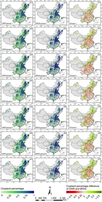
Remote Sens. 2019, 11, 213                                                                           2 of 18

for survival [3]. Croplands also play an important role in the global carbon cycle and regulate the
climate by releasing greenhouse gases (e.g., methane, nitrous oxide). Accurate information on cropland
distribution is thus of great significance for agricultural monitoring, yield estimation, and food security
assessment, and can also inform both climate policymaking and efforts to meet zero hunger of the
sustainable development goals (SDGs) of the United Nations for 2030 [4–6].
     Over the past several decades, remote sensing has become the predominant method for acquiring
large-scale cropland extent information. Some regional and global cropland maps with spatial
resolution varying from 30 m to 1 km have been derived from remote sensing and made freely
available to the public. The widely used global cropland maps include the global land cover database
of the year 2000 (GLC2000) [7], University of Maryland (UMd) land cover layer [8], the Moderate
Resolution Imaging Spectroradiometer land product Collection 5 (MODIS C5) [9], MODIS Cropland
dataset [10], and the 30 m global land cover data product (GlobeLand30) [11]. Cropland mapping
using remote sensing at regional or global scales is generally a massive task that is labor-intensive
and time-consuming. For instance, hundreds of scientists were involved in the development of the
GlobeLand30 over the years of 2010–2014 [11]. Despite the tremendous efforts, these datasets were
found to be inconsistent with each other because of the difference in sensors, classification schemes,
and classification methods [5,12,13]. The substantial uncertainty in these land cover/cropland maps
limits their application in research and management [14–16].
     In order to solve the above issue, synergy approaches have been recently developed to create
hybrid cropland maps by integrating existing cropland datasets [17–20]. These synergy approaches
can be generally classified into two groups: Regression analysis methods and data consistency scoring
methods [5,21]. The former group first establishes a regression relationship between training samples
and input datasets, and then uses it to predict the probability of the occurrence of cropland in the
non-sampled region. The regression models are typically based on a large number of training samples.
Regression analysis has been used to generate hybrid land cover maps at regional and global scales.
Kinoshita et al. [22] created a global land cover and probability map through logistic regression.
See et al. [18] used a logistic geographically weighted regression (GWR) method to establish global
land cover products at 1 km spatial resolution. In addition, Schepaschenko et al. [20] used the GWR
model to produce a global forest cover map. The second group of synergy approaches builds a score
table based on the consistency of the input land-cover products and selects pixels with high confidence
for synergy. For example, Jung et al. [23] developed a fuzzy agreement scoring method to produce a
new joint 1 km global land cover product. Following Jung et al. [23], Fritz et al. [4] used a modified
fuzzy agreement scoring (MFAS) synergy method to generate a synergy cropland map at the global
scale. Lu et al. [5] generated a synergy cropland map of China using a new hierarchical optimization
synergy approach.
     Assessing performance of synergy approaches in an objective manner is fundamental to synergy
cropland mapping. It can help users to select a method for mapping and assess the uncertainties
of results. The most common approach for performance assessment is to compare the accuracies of
synergy results with test samples. For example, Clinton et al. [24] compared nine synergy methods for
the derivation of three global land cover maps, and Lesiv et al. [25] compared five synergy methods
for creating hybrid forest cover maps using the Geo-Wiki [26,27] crowdsourced data. These two
studies indicated that GWR had better performance in global land cover mapping than other synergy
methods. However, the above studies are only limited to comparing various regression analysis
methods, not including data consistency scoring methods. More importantly, these studies only
compared the spatial accuracy of the results and did not analyze the adaptabilities of various input
datasets, training samples, and landscapes.
     To overcome such problems, this study compared and analyzed the advantages, disadvantages,
and regional adaptabilities of regression analysis methods and data consistency scoring methods.
We chose the GWR and MFAS that are the most widely used as the representative methods
respectively [5,21], and used seven satellite-based cropland maps to create synergy cropland maps.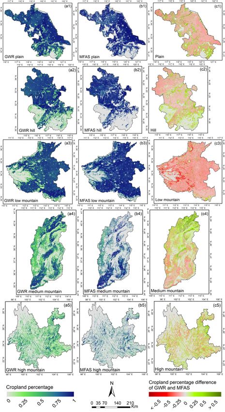
Remote Sens. 2019, 11, 213                                                                                       3 of 18

China is taken as the study area due to its large territory and high agricultural landscape heterogeneity.
Three different experiments are conducted to compare the GWR model and MFAS method in terms of
sample size, quality of input products, and landscapes. Three statistical measures, including overall
accuracy (OA), coefficient of determination (R2 ), and area difference rate (ADR), were calculated to
analyze the results of the synergy mapping.

2. Principles of the two synergy methods

2.1. Geographical Weighted Regression
     GWR is a spatial analytical method employing locational information and smoothing techniques
for regression models, in which regression parameters vary with different geographic locations [28].
Therefore, GWR usually has better simulation results for large areas than other regression methods.
The principle of GWR is that the geographical locations of the independent variables in the regression
and the observations are weighted by distance, and those closer to the studied locations have more
influence on the parameter estimates. The GWR equation can be expressed as follows:
                                                                      n
                                            yi = β 0 ( ui , vi ) +   ∑ βt (ui , vi )Xit + ε i                       (1)
                                                                     t =1

where (ui , vi ) are the coordinates of sample i; β 0 (ui , vi ) is the intercept term; β t (ui , vi ) is a geographical
location function indicating the t-th regression coefficient of sample i; ε i is the random error term of
sample i; Xit is the cropland percentage of t input maps in the training sample i, and yi is the actual
percentage of cropland in training sample i. n is the number of input maps. The estimation of the
regression coefficients is based on a weighted least squares method as shown in the following equation:
                                                                             −1
                                       β t ( ui , vi ) = X T W ( ui , vi ) X      X T W ( u i , v i )Y              (2)

where X is the matrix of the independent variables; X T is the transpose of X; W (ui , vi ) is the spatial
weight matrix whose diagonal elements represent the geographical weights of observations near i; Y is
the matrix of the dependent variables. The adaptive kernel function based on a bi-square distance
decay function is used to obtain the geographical weights. The optimal bandwidth of the bi-square
function is determined by the Akaike Information Criterion (AIC).
     The regression coefficients of the training samples are calculated by GWR, while the regression
coefficients of other pixels are calculated by the inverse distance weighted (IDW) interpolation method.
Finally, the cropland percentage map is calculated using the linear regression as follows:

                             yk = a0(uk ,vk ) + a1(uk ,vk ) × x1(uk ,vk ) + . . . + an(uk ,vk ) × xn(uk ,vk )       (3)

where yk is the cultivated land cover at each location k; (uk , vk ) is the two-dimensional vector of location
k; x1 · · · xn are the percentage of cropland from the individual input maps; a0 and a1 · · · an are the
intercept term and regression coefficients at location k calculated using GWR and IDW interpolation,
respectively; and n is the number of input maps.

2.2. Modified Fuzzy Agreement Scoring
     The logic of the MFAS method is that pixels with greater agreement among existing cropland data
products are more likely to truly be cropland pixels [4,29]. The input maps are firstly ranked by their
accuracy assessment, and then a score table is established for different map combinations according to
the map ranks. The cropland areas from the agricultural statistics are used as the standard to select
pixels with high ranks until the accumulated cropland area is close to the cropland area statistics.
     The input cropland maps are first ranked to create an initial synergy map. Specifically, the training
samples are used to assess the accuracy of each individual cropland map, and the rank of each map is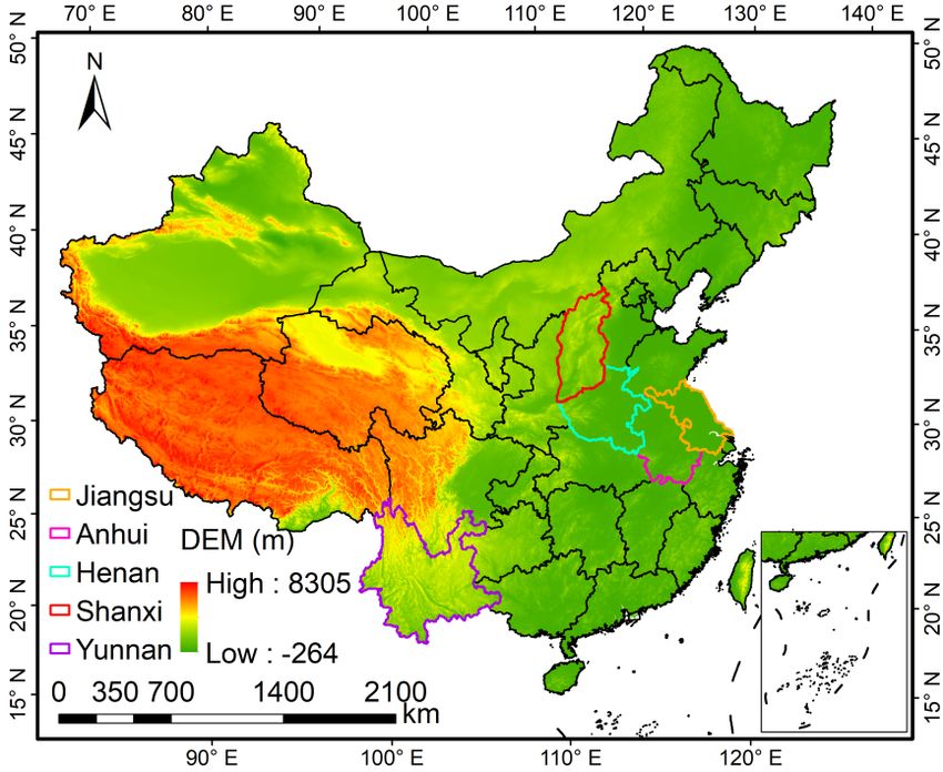
Remote Sens. 2019, 11, x FOR PEER REVIEW 4 of 19
The input cropland maps are first ranked to create an initial synergy map. Specifically, the
Remote Sens. 2019, 11, 213 4 of 18
training samples are used to assess the accuracy of each individual cropland map, and the rank of
each map is determined based on its accuracy (i.e., the higher accuracy indicates a higher rank). A
score table is then
determined basedestablished based
on its accuracy on the
(i.e., thehigher
ranks accuracy
and agreement of ainput
indicates highermaps. For
rank). A example,
score tablewhenis then
five different maps
established basedare on employed,
the ranks and theagreement
values of the score maps.
of input table range from 1 towhen
For example, 32, asfive
shown in Table
different maps
S1are
from the online Supplementary Material. The input maps are transformed
employed, the values of the score table range from 1 to 32, as shown in Table S1 from the online into an initial synergy
map using the score
Supplementary table. The
Material. The input
initialmapssynergy map is then into
are transformed calibrated bysynergy
an initial the “true”
mapcropland
using thearea score
reported
table. Thein the agricultural
initial synergy map statistics. The pixelsbywith
is then calibrated high score
the “true” values
cropland areaare selected
reported in and the total
the agricultural
cropland area
statistics. The ofpixels
these with
pixelshigh
is calculated
score values basedareon the average
selected and thecropland percentage
total cropland area and pixelpixels
of these area. is
The allocation
calculated process
based continues
on the averageuntil the total
cropland cropland
percentage andarea is very
pixel area. close to the trueprocess
The allocation area obtained
continues
from the
until the agricultural
total cropland statistics.
area is very close to the true area obtained from the agricultural statistics.
InInthis research,
this research, thethe
synergy
synergy processing
processing is conducted
is conductedfor each province.
for each For each
province. For province, the
each province,
accuracy of each
the accuracy of input map is
each input mapevaluated
is evaluatedat first
at and
firstthe
andranking of each
the ranking individual
of each individualinputinput
dataset is
dataset
determined. The score table of each province is then established to obtain an
is determined. The score table of each province is then established to obtain an initial synergy map. initial synergy map.
Finally,
Finally,the provincial
the provincial cropland
cropland areas
areas from
from the
theagricultural
agriculturalstatistics areare
statistics used
usedto to
generate
generate thethe
synergy
synergy
cropland
cropland mapmap byby calibrating
calibratingthe initial
the initial synergy
synergy map.
map.
3. 3. Data
Data andand Experiment
Experiment Design
Design
We Wedesigned
designed threecomparison
three comparison experiments
experiments using
using various
various sets
sets ofof training
training samples,
samples, multiple
multiple
cropland
cropland maps
maps with
with different
different accuracy,
accuracy, and
and different
different landscapes
landscapes (Figure
(Figure 1).1).
WeWe chose
chose China
China asasourour
study
study area
area (Figure
(Figure 2).2).
AA total
total of of seven
seven satellite-based
satellite-based cropland
cropland maps
maps at at varying
varying spatial
spatial resolution
resolution
were
were used
used in in this
this study.
study. The
The results
results of of experiments
experiments were
were assessed
assessed and
and compared
compared byby spatial
spatial accuracy,
accuracy,
consistencywith
consistency withcropland
croplandpercentage
percentage of validation
validation samples,
samples,andandconsistency
consistency with cropland
with croplandareaarea
from
the the
from agricultural
agriculturalstatistics.
statistics.
Figure
Figure 1. The
1. The flowchart
flowchart of of
thethe comparison
comparison experiments.
experiments.
Remote Sens. 2019, 11, x; doi: FOR PEER REVIEW www.mdpi.com/journal/remotesensing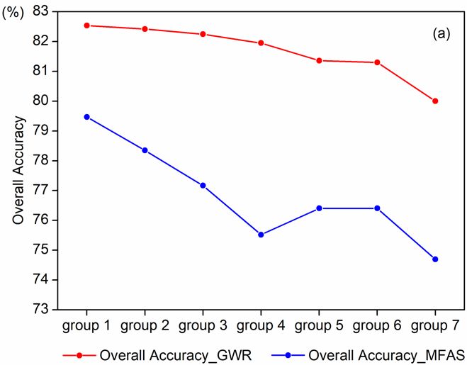
Remote Sens. 2019, 11, 213 5 of 18
Remote Sens. 2019, 11, x FOR PEER REVIEW 5 of 19
Figure 2.
Figure 2. The
Thestudy
studyarea: China
area: and and
China five provinces (Jiangsu,
five provinces Anhui, Anhui,
(Jiangsu, Henan, Shanxi,
Henan, Yunnan). The
Shanxi, Yunnan).
Digital Elevation Model (DEM) represents the landscapes of the study area. Synergy
The Digital Elevation Model (DEM) represents the landscapes of the study area. Synergy cropland cropland
mapping with
mapping with various
various training
trainingsample
samplesizes
sizesand
and synergy
synergy cropland
cropland mapping
mapping withwith different
different satellite-
satellite-based maps were conducted in China. Synergy cropland mapping with various
based maps were conducted in China. Synergy cropland mapping with various landscapes were landscapes
were conducted
conducted in provinces.
in five five provinces.
3.1. Data and
3.1. Data andprocessing
processing
Seven satellite-based
Seven satellite-basedcropland
croplandmaps,maps, including
including GlobeLand30,
GlobeLand30, Climate Change
Climate Change Initiative land land
Initiative
cover product (CCI-LC), MODIS Collection5, MODIS Cropland, GlobCover
cover product (CCI-LC), MODIS Collection5, MODIS Cropland, GlobCover 2009, Unified Cropland, 2009, Unified Cropland,
and the
and the National
Nationallandlanduse/cover
use/cover database
database of of
China
China(NLUD-C)
(NLUD-C) 2010 were
2010 usedused
were for synergy
for synergy cropland
cropland
mapping of
mapping of China
China in in 2010.
2010. The
TheGlobeLand30
GlobeLand30 map mapisisatat30
30mmspatial
spatialresolution
resolutionandandwas wasproduced
producedbased
based
on on Landsat
Landsat and HJ-1 andsatellite
HJ-1 satellite
images images
usingusing a pixel-object-knowledge
a pixel-object-knowledge method
method [30].[30].
TheThe CCI-LC
CCI-LC map is
map is a 300 m global land cover dataset based on the Medium Resolution
a 300 m global land cover dataset based on the Medium Resolution Imaging Spectrometer InstrumentImaging Spectrometer
Instrument (MERIS) time series data from 2008 to 2012 [31]. The MODIS Collection 5 land cover map
(MERIS) time series data from 2008 to 2012 [31]. The MODIS Collection 5 land cover map was
was generated at 500 m spatial resolution based on MODIS bands 1–7 and the enhanced vegetation
generated at 500 m spatial resolution based on MODIS bands 1–7 and the enhanced vegetation index
index (EVI) using a decision tree classification algorithm [9]. The MODIS Cropland map was
(EVI) using a decision tree classification algorithm [9]. The MODIS Cropland map was developed from
developed from multiyear MODIS data with 250 m spatial resolution and cropland area statistics
multiyear MODIS data with 250 m spatial resolution and cropland area statistics using a decision tree
using a decision tree classification algorithm [10]. The GlobCover 2009 map is at 300 m spatial
classification algorithm [10]. The GlobCover 2009 map is at 300 m spatial resolution and was produced
resolution and was produced by European Space Agency and the Université catholique de Louvain
by European
using Space
time series AgencyFine
of MERIS andResolution
the Université
2009 catholique
mosaics [32].deThe
Louvain using time
2014 Unified series Layer
Cropland of MERISis at Fine
Resolution
250 m spatial 2009 mosaicsand
resolution [32].was
Theproduced
2014 Unified Croplandthe
by combining Layer is at
fittest 250 m spatial
products according resolution
to four and
was produced by combining the fittest products according to four dimensions:
dimensions: timeliness, legend, resolution, and confidence [33]. The NLUD-C map was produced timeliness, legend,
resolution,
from Landsat andTM/ETM+
confidence [33]. by
images TheChinese
NLUD-C map was
Academy producedusing
of Sciences fromhuman-machine
Landsat TM/ETM+ images by
interactive
Chinese Academy
interpretation of Sciences using human-machine interactive interpretation [34,35].
[34,35].
These croplandmaps
These cropland mapsarearebased
basedonon different
different mapmap projections,
projections, classification
classification schemes,
schemes, and spatial
and spatial
resolution.
resolution. TheThepreprocessing
preprocessingof ofthese these maps
maps prior
prior to to
thethe synergy
synergy mapping
mapping included
included projection
projection
transformation, cropland
transformation, cropland definition
definition harmonization,
harmonization, and andspatial
spatialresolution
resolutionstandardization.
standardization.These Theseinput
input were
maps mapsfirst
wereprojected
first projected
into the into
samethemap
sameprojection.
map projection.
We then Weharmonized
then harmonized the cropland
the cropland definitions
definitions using the Food and Agriculture Organization (FAO) cropland
using the Food and Agriculture Organization (FAO) cropland definition as the common definition as the common
definition for
definition
the for theThe
seven maps. seven
FAOmaps. The definition
cropland FAO cropland definition
includes includes
arable land arable land crops.
and permanent and permanent
Pure cropland
crops. Pure cropland and mosaic cropland classes were given high and low
and mosaic cropland classes were given high and low weights, respectively [5]. Table S2 from weights, respectively [5]. the
Table S2 from the online Supplementary Material shows the cropland definitions
online Supplementary Material shows the cropland definitions and modified cropland percentage and modified
cropland
of percentage
the input of the input
maps. Finally, maps.were
all maps Finally, all maps were
resampled to 500resampled
m spatialtoresolution
500 m spatial withresolution
the average
with the average cropland percentage.
cropland percentage.
Remote Sens. 2019, 11, x; doi: FOR PEER REVIEW www.mdpi.com/journal/remotesensingRemote Sens. 2019, 11, 213 6 of 18
A total of 2800 cropland samples and 2851 noncropland samples were used for the experiments.
Among them, 443 cropland samples and 1687 noncropland samples were obtained from Tsinghua
University (http://data.ess.tsinghua.edu.cn/). In the collection scheme of samples from Tsinghua
University, the entire globe was partitioned by about 7000 equal area hexagons using DGGRID software,
and 10 samples were selected randomly in each hexagon [36]. The land cover types were identified
by visual interpretation via high resolution images. As there are only 443 cropland samples in China
which is not enough for experiments, the other samples were collected from the study of Lu et al.
(2017). In the sampling frame of Lu et al. (2017), the samples were selected by using the stratified
random sampling method based on the agreement of input cropland maps [5], and their land cover
types were identified by Google Earth images (provided by DigitalGlobe’s WorldView-2 satellite sensor
and obtained from the Google Earth Pro software) circa 2010. For each of these samples (pixels) that
were identified, we estimated the cropland percentage within the 500 m × 500 m pixel using Google
Earth images. In this study, we used a stratified random sampling method to divide training samples
and validation samples. 70% of the total samples were selected randomly for training, and the rest
(847 cropland samples, 848 noncropland samples) were used for validation (Figure S1 from the online
Supplementary Material).
The statistics of cropland area in 2010 were acquired from the project of Second National Land
Survey, the official national statistics in China. The cropland area was estimated based on survey base
maps which were created by remote sensing images, and the definition of cropland was similar to that
used by the FAO. In this research, the cropland area statistics at the province level (Table S3 from the
online Supplementary Material) were used for calibration in the MFAS method.
3.2. Experiment Description
The accuracy of the seven harmonized cropland maps were assessed using the validation samples
(Table 1). The maps with accuracy from high to low are Unified Cropland (#1), GlobeLand30 (#2),
NLUD-C (#3), MODIS Collection 5 (#4), CCI-LC (#5), MODIS Cropland (#6), and GlobCover2009 (#7).
Table 1. Accuracy and consistency with cropland percentages and statistics of the seven harmonized
cropland maps.
Overall R2 between Maps and the R2 between Maps and the
Cropland Maps
Accuracy (%) Cropland Percentage Cropland Area Statistics
Unified Cropland 81.18 0.68 0.79
GlobeLand30 77.76 0.60 0.80
NLUD-C 76.76 0.55 0.83
MODIS Collection5 76.58 0.38 0.74
CCI-LC 75.69 0.36 0.58
MODIS Cropland 71.86 0.27 0.44
GlobCover 2009 69.50 0.23 0.38
3.2.1. Synergy Cropland Mapping with Various Training Sample Sizes
In this experiment, we analyzed the influence of the size of training samples on the two synergy
methods. Seven groups of training samples, including 90%, 70%, 50%, 30%, 10%, 5%, and 1% of the
total training samples were randomly selected (Table 2). In order to achieve best results, we chose
the input map combination with the highest average accuracy (Unified Cropland, GlobeLand30,
and NLUD-C) for synergy cropland mapping. The resulting maps were then used to evaluate the
effects of the training sample size.Remote Sens. 2019, 11, 213 7 of 18
Table 2. The design of the experiment for assessing the influence of the size of training samples for
synergy cropland mapping. The cropland maps used are Unified Cropland (#1), GlobeLand30 (#2),
and NLUD-C (#3).
Samples 1 Samples 2 Samples 3 Samples 4 Samples 5 Samples 6 Samples 7
Proportion of total training sample 90% 70% 50% 30% 10% 5% 1%
Cropland training samples 1777 1383 969 574 176 92 15
Noncropland training samples 1783 1386 1009 613 220 106 25
Validation samples Cropland: 847 Noncropland: 848
Input datasets combination #1, #2, #3
3.2.2. Synergy Cropland Mapping with Different Satellite-Based Maps
In this experiment, we assessed the influence of the quality of the input satellite-based map on the
two synergy methods. All the training samples were employed for GWR and MFAS. We calculated the
average accuracy of each combination of three input maps, and then selected seven groups of input
map combinations, with their average accuracy ranging from high to low (Table 3). The combination
of Unified Cropland, GlobeLand30, and NLUD-C had the highest overall accuracy (78.57%), followed
by the combination of Unified Cropland, MODIS Collection 5, and CCI-LC. The combination including
CCI-LC, MODIS Cropland, and GlobCover2009 had the lowest accuracy (72.35%). The synergy
maps resulting from these experiments were then used to compare and analyze the effects of input
satellite-based maps on synergy cropland mapping.
Table 3. The experiment design of the influence of input satellite-based map quality. The cropland
maps used are Unified Cropland (#1), GlobeLand30 (#2), NLUD-C (#3), MODIS Collection 5 (#4),
CCI-LC (#5), MODIS Cropland (#6), and GlobCover2009 (#7).
Group 1 Group 2 Group 3 Group 4 Group 5 Group 6 Group 7
Input map combination #1, #2, #3 #1, #4, #5 #1, #4, #6 #2, #5, #6 #2, #3, #7 #3, #5, #7 #5, #6, #7
Average accuracy (%) 78.57 77.82 76.54 75.10 74.67 73.98 72.35
Training samples Cropland: 1953 Noncropland: 2003 Total: 3956
Validation samples Cropland: 847 Noncropland: 848
3.2.3. Synergy Cropland Mapping with Various Landscapes
In this experiment, we analyzed the influence of various landscapes on the two synergy
methods. A series of studies showed that landscapes have distinct impacts on land cover/cropland
mapping [12,13,37]. In China, the mountainous areas are usually characterized by heterogeneous
landscapes, while plain areas generally represent homogeneous landscapes. Therefore, we used the
elevation as an indicator to select areas with various landscapes for the comparison between GWR
and MFAS. Chai et al. [38] divided the geomorphologic forms into plain (1500 m). According
to this standard, we chose five provinces including Jiangsu, Anhui, Henan, Shanxi, and Yunnan
(Figure 2) for which mean elevations are shown in Table 4. All the training samples and input datasets
were employed for the synergy mapping based on both GWR and MFAS. Then, results of the five
provinces were extracted and assessed by 100 validation samples in each region.
Table 4. The experiment design of the influence of various landscapes.
Test 1 Test 2 Test 3 Test 4 Test 5
Province Jiangsu Anhui Henan Shanxi Yunnan
Landscape Plain Hill Low mountain Medium mountain High mountain
Average DEM (m) 13.26 119.01 247.59 1160.68 1889.64
Validation Cropland 74 70 70 60 35
samples Noncropland 26 30 30 40 65Remote Sens. 2019, 11, 213 8 of 18
3.3. Performance Assessment
The performance assessment included overall accuracy (OA), coefficient of determination (R2 ),
and area difference rate (ADR), which were mainly calculated in ENVI software and IDL (Interactive
Data Language). The overall accuracy (OA) was used to assess the accuracy of the synergy results.
The overall accuracy is calculated as follows:
nc
OA = × 100% (4)
n
where nc is the number of pixels that were correctly classified, and n is the total number of pixels.
According to Pontius and Millones (2010), we did not choose the Kappa coefficient to assess accuracy
because it was misleading or flawed for practical applications [39].
The coefficient of determination (R2 ) was used to evaluate the correlation between the
fusion cropland percentage and the cropland percentage identified from high-resolution images
(i.e., the cropland percentage from the Google Earth), and the correlation between the fusion provincial
cropland area and the cropland area statistical data. The area difference rate (ADR) was used to assess
the degree of difference between a single fusion cropland area and a real cropland area. ADR is
calculated as follows:
cp − sp
ADR = × 100% (5)
sp
where c p is the cropland area of a single province p estimated by the synergy map and s p is the
cropland area statistical data of the province p as the reference.
4. Results
4.1. Influence of Training Samples
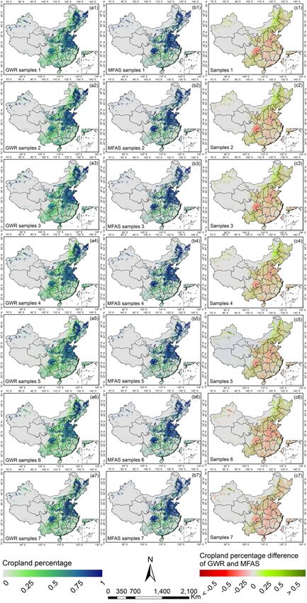
The two synergy methods (GWR and MFAS) were employed for cropland mapping with multiple
sets of training samples (Table 2). The two methods led to similar cropland distributions but exhibited
large differences in cropland percentage (Figure 3). The cropland percentage predicted by MFAS
was higher than that by GWR in some regions such as Sichuan Basin, Hunan Province, and North
China Plain. This pattern was more obvious when the number of training samples decreased.
By contrast, the cropland percentage predicted by GWR was higher than that by MFAS in Inner
Mongolia and Xinjiang.
We compared spatial accuracy, consistency with the cropland percentage identified from
high-resolution images, and consistency with the statistics to assess how the performances of GWR and
MFAS varied with the size of training samples (Figure 4). The overall accuracy of the GWR synergy
results slightly decreased with the reduction in the number of training samples, particularly when the
number of training samples was less than 10% of the original samples. The training sample size had no
significant effects on the overall accuracy of MFAS synergy results (Figure 4a). For the consistency with
the cropland percentage identified from high-resolution images, when the training samples decreased,
there was a slight reduction in R2 between the GWR synergy results and the cropland percentage
identified from high-resolution images. The impact of training samples on the R2 between the MFAS
synergy results and the cropland percentage identified from high-resolution images was small. For the
consistency with cropland area statistics, as the training samples decreased, the R2 between the GWR
synergy results and the cropland area statistical data gradually increased. The R2 values between the
MFAS synergy results and cropland area statistical data were stable and higher than those of the GWR
synergy results (Figure 4b).Remote Sens. 2019, 11, 213 9 of 18
Remote Sens. 2019, 11, x FOR PEER REVIEW 9 of 19
Figure 3. Synergy cropland results of: Geographically weighted regression
Remote Sens. 2019, 11, x; doi: FOR PEER REVIEW
(GWR) (left panel) and
www.mdpi.com/journal/remotesensing
modified fuzzy agreement scoring (MFAS) (middle panel) and their difference images (right panel).
Panels from top to bottom represent synergy results with various sample sets as shown in Table 2.cropland percentage identified from high-resolution images. The impact of training samples on the
R2 between the MFAS synergy results and the cropland percentage identified from high-resolution
images was small. For the consistency with cropland area statistics, as the training samples
decreased, the R2 between the GWR synergy results and the cropland area statistical data gradually
increased. The R2 values between the MFAS synergy results and cropland area statistical data were
Remote Sens. 2019, 11, 213 10 of 18
stable and higher than those of the GWR synergy results (Figure 4b).
Figure4.
Figure 4. Performance
Performance assessment
assessment and comparisons
and including
comparisons spatialspatial
including accuracy (a), consistency
accuracy with
(a), consistency with
cropland percentages,
cropland percentages, and
andconsistency with
consistency cropland
with area area
cropland from from
the statistics using various
the statistics sample sample
using various
sets(b).
sets (b).
4.2.Influence
4.2. Influence of Satellite-Based
Satellite-BasedMaps
Maps
Weselected
We selected three
threeofofthe
theseven maps
seven to form
maps seven
to form combinations
seven with various
combinations average average
with various accuracy.accuracy.
These combinations of satellite-based maps were applied for GWR and MFAS to generate synergy
These combinations of satellite-based maps were applied for GWR and MFAS to generate synergy
cropland maps (Figure 5). With the decrease in the average accuracy of the input maps, the
cropland maps (Figure 5). With the decrease in the average accuracy of the input maps, the difference in
difference in the cropland percentage predicted using the two methods increased, particularly in
the cropland
Shaanxi percentage
Province and nearpredicted using
the border the two
of Shanxi methods
and increased,
Inner Mongolia particularly
Provinces in5c1
(Figure Shaanxi
to c7).Province
and
When the average accuracy of the input maps was the lowest, the difference between the the
near the border of Shanxi and Inner Mongolia Provinces (Figure 5c1–c7). When two average
accuracy
methodsof thethe
was input maps was the lowest, the difference between the two methods was the largest.
largest.
It is clear that the overall accuracy of the two synergy results decreased as the average accuracy
of the input map combination decreased, and MFAS was more sensitive to the quality of input maps
compared with GWR (Figure 6a). The R2 values between both synergy methods and the cropland
percentage identified from high-resolution images decreased with the reduction in the average accuracy
of the input map combination. The average accuracy of the input map had significantly higher effects
on the MFAS synergy results than on the GWR synergy results (Figure 6b). When the average accuracy
Remote Sens. 2019, 11, x; doi: FOR PEER REVIEW www.mdpi.com/journal/remotesensing
of the dataset decreased, the R2 between the GWR synergy results and cropland area statistical data
gradually decreased. However, the R2 between the MFAS synergy results and cropland area statistical
data remained at high levels all the time and only slightly changed (Figure 6b).Remote Sens. 2019, 11, 213 11 of 18
Remote Sens. 2019, 11, x FOR PEER REVIEW 11 of 19
Figure 5. Synergy
Remote Sens. cropland
2019, 11, x; mapsREVIEW
doi: FOR PEER of GWR (left panel) and MFAS (middle panel) and their difference
www.mdpi.com/journal/remotesensing
images (right panel). Panels from top to bottom represent synergy results with various average
accuracy of input satellite-based map combinations as shown in Table 3.accuracy of the input map combination. The average accuracy of the input map had significantly
higher effects on the MFAS synergy results than on the GWR synergy results (Figure 6b). When the
average accuracy of the dataset decreased, the R2 between the GWR synergy results and cropland
area statistical data gradually decreased. However, the R2 between the MFAS synergy results and
cropland area statistical data remained at high levels all the time and only slightly changed (Figure
Remote Sens. 2019, 11, 213 12 of 18
6b).
Figure 6.
Figure 6. Performance
Performanceassessment
assessmentandand
comparisons
comparisons including spatial
including accuracy
spatial (a), consistency
accuracy with
(a), consistency with
cropland percentage,
cropland percentage,and
andconsistency with
consistency statistics
with using
statistics inputinput
using satellite-based map combinations
satellite-based of
map combinations of
various average accuracy (b).
various average accuracy (b).
4.3. Influence
4.3. Influence ofofVarious
VariousLandscapes
Landscapes
To evaluate
To evaluate the
theeffects
effectsofof
different landscapes
different on the
landscapes on synergy mapping
the synergy of the of
mapping two methods,
the we
two methods, we
selected five regions of different landscapes for comparative experiments. In plain, hill,
selected five regions of different landscapes for comparative experiments. In plain, hill, and low and low
mountain areas, the percentage of cropland predicted by MFAS was slightly higher than that by
mountain areas, the percentage of cropland predicted by MFAS was slightly higher than that by GWR
GWR (Figure 7). In medium mountain and high mountain areas where the average elevation is
(Figure 7). In medium mountain and high mountain areas where the average elevation is above 500 m,
above 500 m, the percentage of cropland predicted by GWR was gradually higher than that by
the percentage of cropland predicted by GWR was gradually higher than that by MFAS.
MFAS.
This shows that with increases in average elevation, the overall accuracy of the GWR synergy
maps decreased (Figure 8a). At elevations higher than 1500 m, the overall accuracy of GWR sharply
decreased. The overall accuracy of the MFAS also decreased with the increase in average elevation.
When the elevation is higher than 200 m, the overall accuracy of MFAS synergy maps dramatically
decreased. The variation trends in R2 between both synergy results and the cropland percentage
identified from high-resolution images (Figure 8b) were consistent with the overall accuracy trends
(Figure 8a). The area difference rate between the cropland area of the GWR synergy results and
cropland area statistical data was higher than that between the cropland area of the MFAS synergy
results and cropland area statistical data. As the average elevation increased, the gap between the area
difference rates of two approaches also gradually increased. Particularly for the GWR model, when the
elevation is higher than 500 m, the area difference rate obviously increased (Figure 8c). However,
Remote Sens. 2019, 11, x; doi: FOR PEER REVIEW www.mdpi.com/journal/remotesensing
the effect of various landscapes on the area difference rates between the cropland area of the MFAS
synergy results and cropland area statistical data was relatively low and not obvious.Remote Sens. 2019, 11, 213 13 of 18
Remote Sens. 2019, 11, x FOR PEER REVIEW 13 of 19
Figure 7. Synergy
Synergy cropland
cropland maps of GWR
GWR (left
(left panel)
panel) and
and MFAS
MFAS (middle panel) and their difference
difference
images (right panel). Panels
Panels from
from top
top to
to bottom
bottom represent
represent synergy results with various landscapes as
shown in Table 4.
Remote Sens. 2019, 11, x; doi: FOR PEER REVIEW www.mdpi.com/journal/remotesensing(Figure 8a). The area difference rate between the cropland area of the GWR synergy results and
cropland area statistical data was higher than that between the cropland area of the MFAS synergy
results and cropland area statistical data. As the average elevation increased, the gap between the
area difference rates of two approaches also gradually increased. Particularly for the GWR model,
when the elevation is higher than 500 m, the area difference rate obviously increased (Figure 8c).
However,
Remote the effect
Sens. 2019, of various landscapes on the area difference rates between the cropland area of
11, 213 14 of 18
the MFAS synergy results and cropland area statistical data was relatively low and not obvious.
Figure Performance
8. Performance
Figure 8. assessment
assessment and and comparisons
comparisons including
including spatial accuracy
spatial accuracy (a), consistency
(a), consistency with with
cropland percentage
cropland percentage (b),
(b), and
and consistency
consistency withwith statistics
statistics (c)various
(c) using using various landscapes.
landscapes.
5.5.Discussion
Discussion
The GWR
The GWR model
modelis isa regression
a regression analysis basedbased
analysis on theon cropland percentage
the cropland of the training
percentage of the training
samples [18,40], while the MFAS method mainly depends on the consistency
samples [18,40], while the MFAS method mainly depends on the consistency of input datasets, of input datasets, and and the
the training samples only play an auxiliary role [29]. We conducted three experiments to analyze the
training samples only play an auxiliary role [29]. We conducted three experiments to analyze the
influence of the size of training samples, the quality of satellite-based cropland maps, and changes in
influence of the size of training samples, the quality of satellite-based cropland maps, and changes
landscapes on the performance of the two methods. GWR generally has higher overall accuracy and
inbetter
landscapes on the
consistency performance
of cropland of thewhile
percentage, two MFAS
methods. GWRconsistency
has better generally withhas higher
croplandoverall
area accuracy
and better
statistics. consistency of cropland percentage, while MFAS has better consistency with cropland
area statistics.
Training samples are essential input data for the synergy methods. GWR is more sensitive to
and Training
dependent on training
samples samples than
are essential inputMFAS. Forthe
data for GWR, the more
synergy trainingGWR
methods. samples, the more
is more sensitive to and
accurate the synergy map is and the closer the predicted value
dependent on training samples than MFAS. For GWR, the more training samples, the is to the real value. Previous studies
more accurate
showed that the representativeness in quality and quantity of training samples, as well as their
the synergy map is and the closer the predicted value is to the real value. Previous studies showed that
spatial homogeneity, were quite important for the GWR model [20,41,42]. We also found that when
the representativeness in quality and quantity of training samples, as well as their spatial homogeneity,
the samples were relatively sufficient, the overall accuracy of the GWR synergy maps was slightly
were
higherquite
than important for the
that of the MFAS GWR maps.
synergy model [20,41,42].
However, when We thealso found
number that when
of training the was
samples samples were
relatively
very small,sufficient,
the overallthe overall
accuracy of accuracy of the GWR
the GWR synergy maps synergy
was lowermaps wasof
than that slightly
MFAS. higher
With thethan that of
the MFASofsynergy
number maps. However,
training samples decreasing,when the number
the overall accuracyofoftraining
the GWRsamples
maps and was
the very
MFASsmall,
maps the overall
decreasedofby
accuracy the3.60%
GWRand 1.36%,maps
synergy respectively.
was lowerGWR wasthat
than slightly
of MFAS. more With
sensitive to changes
the number in the samples
of training
number of training
decreasing, samples
the overall than MFAS.
accuracy of the GWR maps and the MFAS maps decreased by 3.60% and
The quality of input
1.36%, respectively. GWR was maps hasslightly
a significant
moreimpact on both
sensitive methods, in
to changes particularly
the number on MFAS. The samples
of training
MFAS method is based on the data consistency [4,29]. Previous studies have shown that the quality
than MFAS.
of the input maps is important for synergy methods based on data consistency [5,29,43]. The
The quality
improvement of quality
in the input maps of input has a significant
datasets impact
can improve the on both methods,
accuracy particularly
of the resulting synergy on MFAS.
The MFAS method is based on the data consistency [4,29]. Previous
maps [29]. Similarly, we found that the quality of the input maps influenced the accuracy of studies have shown
the that the
quality of the input maps is important for synergy methods based on data consistency [5,29,43].
Remote Sens. 2019, 11, x; doi: FOR PEER REVIEW www.mdpi.com/journal/remotesensing
The improvement in the quality of input datasets can improve the accuracy of the resulting synergy
maps [29]. Similarly, we found that the quality of the input maps influenced the accuracy of the
MFAS synergy maps (Figure 5). Our results indicated that as the quality of the input maps decreased,
the overall accuracy of the MFAS and GWR synergy maps decreased by 4.78% and 2.53%, respectively.
The GWR method was less affected because the cropland percentage of the training samples was
directly used.
The landscape is another important factor influencing the performance of the two synergy
methods. Our results showed that the accuracy of the MFAS synergy maps was significantly affected
by landscapes when the elevation is higher than 200 m. The GWR synergy maps were significantly
affected only when the elevation is above 1500 m. The quality of the training samples and input maps
was related to the landscape pattern. In heterogeneous regions with high elevation, the croplands are
generally fragmented, and the consistency of the input satellite-based maps is typically lower [13].
Our results showed that MFAS was more sensitive to the changes in landscape. In the absence of higher
resolution and more accurate input cropland maps, GWR was better than MFAS for heterogeneous
areas. Lesiv et al. [25] also indicated that, in global forest mapping, GWR was more suited to regions
with highly fragmented landscapes than other methods.Remote Sens. 2019, 11, 213 15 of 18
Compared to the GWR model, the MFAS method can generate synergy maps with a higher
correlation with the cropland statistics. That is because MFAS uses the statistics data to calibrate the
initial synergy maps, while the GWR model only considers the spatial distribution of cropland and
does not involve the distribution of cropland areas. Schepaschenko et al. [20] compared a “best guess”
hybrid global forest map by GWR and a hybrid global forest map calibrated with FAO FRA (Forest
Resource Assessment) statistics. Their research showed that at the national scale, there were some
differences between forest area based on GWR and forest area calibrated by FAO statistics partly
because FAO FRA considers forest as land use rather than land cover [20]. Similarly, GWR considers
cropland as land cover, while MFAS considers cropland as land use. It should be noted that when the
number of the training samples decreased, the correlation between the GWR synergy maps and the
cropland statistics increased. The reason is that the three input datasets used for synergy are highly
correlated with statistical data. When the number of training samples decreased, the influence of
input maps on the fusion results became larger, the prediction results were closer to the input maps
which were used for regression, and the correlation between the GWR synergy result and the statistical
data increased.
Cropland percentage predicted by the GWR has higher consistency with the cropland percentage
identified from high-resolution image, compared with MFAS. GWR uses cropland percentage samples
for regression, while MFAS employs the agreement of input maps to conduct experiments. In the MFAS
method, the samples are only used to assess the overall accuracy of the input maps and to establish a
detailed scoring table. However, GWR generally overestimated cropland percentage, such as some
areas in the south and northwest of China. In these areas, the cropland is relatively fragmented
and scarce [44]. Meanwhile, in the GWR model, regression parameters depend on geographical
locations [28], and those pixels closer to croplands are more likely to be predicted as cropland areas.
Many rivers and lakes are usually surrounded by croplands because of sufficient water supply for
irrigation. The cropland percentage of those pixels at the junction of croplands and rivers/lakes
was overestimated.
Method selection is dependent on the input data, landscape, and application purpose. The input
data is the vital baseline information for synergy mapping. Because GWR is more dependent on
training samples, when training samples are insufficient, MFAS is a better choice. For homogeneous
regions, the input cropland products usually have higher accuracies and better consistencies. Therefore,
MFAS is also a good alternative because of its easier and faster operation. For heterogeneous regions,
GWR is a better choice because it outperforms other methods [25]. MFAS can generate a synergy
map which has higher correlation with cropland statistics; therefore, this method is recommended
for synergy map applications that require accuracy cropland area, such as yield estimation [45] and
crop distribution mapping [46]. Meanwhile, for some applications, such as cropland fragmentation
analysis [47], GWR is suitable to generate synergy maps because of its accurate cropland percentage.
In this study, we only compared the two synergy methods GWR and MFAS. In the future, we will
make more comparison experiments, including Naive Bayes and Logistic Regression among others,
to provide more references for method selection.
6. Conclusions
Identifying the advantages and limitations of different synergy methods is critical for generating
accurate spatial distribution information for synergy cropland mapping. In this study, we assessed
and compared the influences of the size of training samples, quality of satellite-based cropland maps,
and changes in landscapes on the performance of two synergy methods: MFAS and GWR. We also
analyzed the advantages, disadvantages, and regional adaptabilities of regression analysis methods
and data consistency scoring methods. When the number of training samples was relatively large,
the GWR method had a higher overall accuracy than the MFAS method. The MFAS method was less
dependent on the samples, and thus it is more suitable where the number of samples is relatively small.
The quality of the satellite-based maps influenced both methods, particularly MFAS. Furthermore,Remote Sens. 2019, 11, 213 16 of 18
GWR was less sensitive to changes in landscapes than MFAS. Cropland areas estimated by MFAS were
more correlated with cropland area statistical data, while the cropland percentage predicted by GWR
was closer to the values as identified from high-resolution images in magnitude. The GWR model is
more suitable for regions with heterogeneous landscapes such as hills and low mountain areas, but the
premise is that the cropland is more widely distributed. On the contrary, MFAS is more suitable for
regions with homogeneous landscapes such as plain areas. MFAS is adequate for producing a global or
regional large-scale cropland map that can be used in a global economic, biophysical, and other land
use model, because it deals with cropland maps as land use types. If the GWR maps are applied for
land use models, calibration by statistical data (such as FAO) is necessary. MFAS is more economical
than GWR, because it is less dependent on sample data and computing resources.
Supplementary Materials: The following are available online at http://www.mdpi.com/2072-4292/11/3/213/s1,
Figure S1: Distribution of training and validation samples, Table S1: The score table of Modified Fuzzy Agreement
Scoring method (5 input maps); Table S2: Cropland definitions and modified cropland percentages of input maps;
Table S3: Provincial statistical data of cropland.
Author Contributions: D.C., M.L., Q.Z. and W.W. conceived and designed the experiments. D.C., M.L. and Y.W.
performed the experiments. D.C., M.L., J.X. and Y.R. analyzed the data. All authors contributed to the writing of
this paper.
Funding: This research was funded by the National Natural Science Foundation of China (41871356), the National
Key Research and Development Program of China (2017YFE0104600), Fundamental Research Funds for Central
Non-profit Scientific Institution (No. 1610132018017) and by the Elite Youth Program of Chinese Academy of
Agricultural Sciences.
Acknowledgments: The Agricultural Land System group at AGRIRS provided valuable support throughout
the research. We are grateful to the anonymous reviewers and academic editor for their valuable suggestions
and comments.
Conflicts of Interest: The authors declare no conflict of interest.
References
1. Foley, J.A.; Ramankutty, N.; Brauman, K.A.; Cassidy, E.S.; Gerber, J.S.; Johnston, M.; Mueller, N.D.;
O’Connell, C.; Ray, D.K.; West, P.C.; et al. Solutions for a cultivated planet. Nature 2011, 478, 337–342.
[CrossRef] [PubMed]
2. Kearney, J. Food consumption trends and drivers. Philos. Trans. R. Soc. B 2010, 365, 2793–2807. [CrossRef]
[PubMed]
3. Godfray, H.; Beddington, J.; Crute, I.; Haddad, L.; Lawrence, D.; Muir, J.; Pretty, J.; Robinson, S.; Thomas, S.;
Toulmin, C. Food security: The challenge of feeding 9 billion people. Science 2010, 327, 812–818. [CrossRef]
[PubMed]
4. Fritz, S.; See, L.; Mccallum, I.; You, L.; Bun, A.; Moltchanova, E.; Duerauer, M.; Albrecht, F.; Schill, C.;
Perger, C.; et al. Mapping global cropland and field size. Glob. Chang. Biol. 2015, 21, 1980–1992. [CrossRef]
5. Lu, M.; Wu, W.; You, L.; Chen, D.; Zhang, L.; Yang, P.; Tang, H. A synergy cropland of china by fusing
multiple existing maps and statistics. Sensors 2017, 17, 1613. [CrossRef] [PubMed]
6. Stansfield, J. The United Nations sustainable development goals (SDGs): A framework for intersectoral
collaboration. Whanake Pac. J. Community Dev. 2017, 3, 38–49.
7. Bartholome, E.; Belward, A.S. GLC2000: A new approach to global land cover mapping from earth
observation data. Int. J. Remote Sens. 2005, 26, 1959–1977. [CrossRef]
8. Hansen, M.; Defries, R.; Townshend, J.; Sohlberg, R. Global land cover classification at 1 km spatial resolution
using a classification tree approach. Int. J. Remote Sens. 2000, 21, 1331–1364. [CrossRef]
9. Friedl, M.; Sulla-Menashe, D.; Tan, B.; Schneider, A.; Ramankutty, N.; Sibley, A.; Huang, X. MODIS collection
5 global land cover: Algorithm refinements and characterization of new datasets. Remote Sens. Environ. 2010,
114, 168–182. [CrossRef]
10. Pittman, K.; Hansen, M.; Beckerreshef, I.; Potapov, P.; Justice, C. Estimating global cropland extent with
multi-year MODIS data. Remote Sens. 2010, 2, 1844–1863. [CrossRef]Remote Sens. 2019, 11, 213 17 of 18
11. Chen, J.; Chen, J.; Liao, A.; Cao, X.; Chen, L.; Chen, X.; Peng, S.; Han, G.; Zhang, H.; He, C.; et al. Concepts
and key techniques for 30 m global land cover mapping. Acta Geod. Cartogr. Sinica 2014, 43, 551–557.
(In Chinese)
12. Wu, W.; Shibasaki, R.; Yang, P.; Zhou, Q.; Tang, H. Remotely sensed estimation of cropland in China:
A comparison of the maps derived from four global land cover datasets. Can. J. Remote Sens. 2008, 34,
467–479. [CrossRef]
13. Lu, M.; Wu, W.; Zhang, L.; Liao, A.; Peng, S.; Tang, H. A comparative analysis of five global cropland datasets
in China. Sci. China Earth Sci. 2016, 59, 2307–2317. [CrossRef]
14. Congalton, R.; Gu, J.; Yadav, K.; Ozdogan, M. Global land cover mapping: A review and uncertainty analysis.
Remote Sens. 2014, 6, 12070–12093. [CrossRef]
15. Yu, L.; Wang, J.; Clinton, N.; Xin, Q.; Zhong, L.; Chen, Y.; Gong, P. FROM-GC: 30 m global cropland extent
derived through multisource data integration. Int. J. Digit. Earth 2013, 6, 521–533. [CrossRef]
16. Liang, L.; Gong, P. Evaluation of global land cover maps for cropland area estimation in the conterminous
United States. Int. J. Digit. Earth 2015, 8, 102–117. [CrossRef]
17. Castanedo, F. A review of data fusion techniques. Sci. World J. 2013, 2013, 704504. [CrossRef]
18. See, L.; Schepaschenko, D.; Lesiv, M.; McCallum, I.; Fritz, S.; Comber, A.; Perger, C.; Schill, C.; Zhao, Y.;
Maus, V.; et al. Building a hybrid land cover map with crowdsourcing and geographically weighted
regression. ISPRS J. Photogramm. Remote Sens. 2015, 103, 48–56. [CrossRef]
19. Verburg, P.; Neumann, K.; Nol, L. Challenges in using land use and land cover data for global change studies.
Glob. Chang. Biol. 2011, 17, 974–989. [CrossRef]
20. Schepaschenko, D.; See, L.; Lesiv, M.; Mccallum, I.; Fritz, S.; Salk, C.; Moltchanova, E.; Perger, C.;
Shchepashchenko, M.; Shvidenko, A.; et al. Development of a global hybrid forest mask through the
synergy of remote sensing, crowdsourcing and FAO statistics. Remote Sens. Environ. 2015, 162, 208–220.
[CrossRef]
21. Chen, D.; WU, W.; Lu, M.; Hu, Q.; Zhou, Q. Progresses in land cover data reconstruction method based on
multi-source data fusion. Chin. J. Agric. Resour. Reg. Plan. 2016, 37, 62–70. (In Chinese)
22. Kinoshita, T.; Iwao, K.; Yamagata, Y. Creation of a global land cover and a probability map through a new
map integration method. Int. J. Appl. Earth Obs. Geoinf. 2014, 28, 70–77. [CrossRef]
23. Jung, M.; Henkel, K.; Herold, M.; Churkina, G. Exploiting synergies of global land cover products for carbon
cycle modeling. Remote Sens. Environ. 2006, 101, 534–553. [CrossRef]
24. Clinton, N.; Yu, L.; Gong, P. Geographic stacking: Decision fusion to increase global land cover map accuracy.
Glob. Land Cover Mapp. Monit. 2015, 103, 57–65. [CrossRef]
25. Lesiv, M.; Moltchanova, E.; Schepaschenko, D.; See, L.; Shvidenko, A.; Comber, A.; Fritz, S. Comparison of
data fusion methods using crowdsourced data in creating a hybrid forest cover map. Remote Sens. 2016, 8,
261. [CrossRef]
26. Fritz, S.; McCallum, I.; Schill, C.; Perger, C.; Grillmayer, R.; Achard, F.; Kraxner, F.; Obersteiner, M.
Geo-wiki.org: The use of crowdsourcing to improve global land cover. Remote Sens. 2009, 1, 345–354.
[CrossRef]
27. Fritz, S.; McCallum, I.; Schill, C.; Perger, C.; See, L.; Schepaschenko, D.; van der Velde, M.; Kraxner, F.;
Obersteiner, M. Geo-wiki: An online platform for improving global land cover. Environ. Model. Softw. 2012,
31, 110–123. [CrossRef]
28. Fotheringham, A.S.; Charlton, M.E.; Brunsdon, C. Geographically weighted regression: A natural evolution
of the expansion method for spatial data analysis. Environ. Plan. A 1998, 30, 1905–1927. [CrossRef]
29. Fritz, S.; You, L.; Bun, A.; See, L.; Mccallum, I.; Schill, C.; Perger, C.; Liu, J.; Hansen, M.; Obersteiner, M.
Cropland for sub-saharan Africa: A synergistic approach using five land cover data sets. Geophys. Res. Lett.
2011, 38, 155–170. [CrossRef]
30. Chen, J.; Chen, J.; Liao, A.; Cao, X.; Chen, L.; Chen, X.; He, C.; Han, G.; Peng, S.; Lu, M.; et al. Global land
cover mapping at 30 m resolution: A POK-based operational approach. ISPRS J. Photogramm. Remote Sens.
2015, 103, 7–27. [CrossRef]
31. Defourny, P.; Kirches, G.; Brockmann, C.; Boettcher, M.; Peters, M.; Bontemps, S.; Lamarche, C.; Schlerf, M.;
Santoro, M. Land Cover CCI: Product User Guide Version 2. Available online: http://maps.elie.ucl.ac.be/
CCI/viewer/download/ESACCI-LC-PUG-v2.5.pdf (accessed on 8 February 2018).You can also read