The Light Source Metaphor Revisited-Bringing an Old Concept for Teaching Map Projections to the Modern Web - MDPI
←
→
Page content transcription
If your browser does not render page correctly, please read the page content below
Article

The Light Source Metaphor Revisited—Bringing an
Old Concept for Teaching Map Projections to the
Modern Web
Magnus Heitzler 1,*, Hans-Rudolf Bär 1, Roland Schenkel 2 and Lorenz Hurni 1
 1 Institute of Cartography and Geoinformation, ETH Zurich, 8049 Zurich, Switzerland;
   hbaer@ethz.ch (H.-R.B.); lhurni@ethz.ch (L.H.)
 2 ESRI Switzerland, 8005 Zurich, Switzerland; roland.schenkel@gmail.com

 * Correspondence: heitzler@karto.baug.ethz.ch

 Received: 28 February 2019; Accepted: 24 March 2019; Published: 28 March 2019

 Abstract: Map projections are one of the foundations of geographic information science and
 cartography. An understanding of the different projection variants and properties is critical when
 creating maps or carrying out geospatial analyses. The common way of teaching map projections in
 text books makes use of the light source (or light bulb) metaphor, which draws a comparison
 between the construction of a map projection and the way light rays travel from the light source to
 the projection surface. Although conceptually plausible, such explanations were created for the
 static instructions in textbooks. Modern web technologies may provide a more comprehensive
 learning experience by allowing the student to interactively explore (in guided or unguided mode)
 the way map projections can be constructed following the light source metaphor. The
 implementation of this approach, however, is not trivial as it requires detailed knowledge of map
 projections and computer graphics. Therefore, this paper describes the underlying computational
 methods and presents a prototype as an example of how this concept can be applied in practice. The
 prototype will be integrated into the Geographic Information Technology Training Alliance
 (GITTA) platform to complement the lesson on map projections.

 Keywords: map projections; computer graphics; visualization; 3D; education; teaching; multimedia;
 open educational resources

1. Introduction
     Map projections are a key concept in cartography and geographic information science. Choosing
an inappropriate map projection may cause severely flawed results when carrying out geospatial
analyses (e.g., when buffering in an inappropriate projected coordinate system [1]) or may distort a
map reader’s view on the world when exploring a thematic or topographic map. Hence, a thorough
understanding of the construction process and map properties is important. Mapping software
typically implements the projection process as a set of equations that can be applied to a point in
geographic coordinates to obtain its projected coordinates. Examples for this approach can be found
in kartograph.js [2], d3.js [3], or Flex Projector [4]. However, educational resources tend to follow a
more figurative approach to explain the underlying geometrical meaning of the projection process.
This construction process typically starts with a projection center that can be imagined as a light
source (or light bulb) placed in the proximity of (or within) the globe and emitting light in all
directions. In the simplest case, the light source has the shape of a point, but other geometries exist
as well. Light rays pass through the globe, casting the colors at their intersection points on the globe's
surface onto the projection surface (usually a plane, cone or cylinder).
ISPRS Int. J. Geo-Inf. 2019, 8, 162; doi:10.3390/ijgi8040162                      www.mdpi.com/journal/ijgi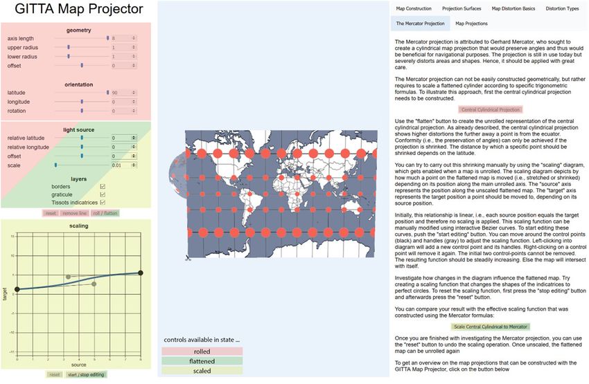
ISPRS Int. J. Geo-Inf. 2019, 8, 162                                                                         2 of 10

      Figure 1 shows three examples of how map projections may be constructed this way. Figure 1A
explains the construction of the gnomonic azimuthal projection by depicting light rays from the light
source in all directions (indicated by arrows) to hit the projection plane. The resulting map is depicted
below, showing distorted shapes of land areas. Figure 1B depicts the construction of the central conic
projection by indicating a projection cone touching the globe with the resulting unrolled map shown
below. Figure 1C intends to illustrate the different positions of the parallels for the central cylindrical
and the Mercator projection implying that an additional non-linear scaling is required to realize the
desired projection. There are numerous resources that show similar depictions, either on the web
(e.g., References [5,6]) or in printed textbooks (e.g., References [7,8]).

      Figure 1. Examples for educational resources following the light source metaphor when explaining map
      projections: (A) gnomonic azimuthal projection (https://commons.wikimedia.org/wiki/File:Comparison
      _azimuthal_projections.svg, CC BY-SA 3.0, accessed 15.02.2019); (B) central conic projection (Weisstein,
      Eric     W.      “Conic      Projection.”     From     MathWorld—A          Wolfram     Web    Resource.
      http://mathworld.wolfram.com/ConicProjection.html, © 1999–2019 Wolfram Research, Inc., accessed
      15.03.2019); (C) central cylindrical projection and Mercator projection (https://commons.wikimedia.org/
      wiki/File:Mercator_and_central_cylindrical.png, Public Domain, accessed 15.02.2019).

     These illustrations have several limitations. Firstly, each illustration shows only snapshots of the
construction process. There is still considerable mental work involved to understand the transition
from the projection concept to the resulting map. Secondly, static images only provide one view on
the construction process. It is not possible to obtain different views to get a comprehensive
understanding of the mapping process. Thirdly, exploring different configurations of these objects is
not possible as this would require interactive adjustments of the light source, projection surface,
basemap, etc. We argue that such interactivity allows improving the understanding of how different
map projections relate to each other. The authors are not aware of any interactive visualization tool,
which allows constructing map projections following an implementation of the light source
metaphor.
     These limitations can be overcome if interactive visualization methods are provided. The
computational concepts and how they can be implemented to create a fully functional web
application are the main contributions of this paper. The concepts are applicable for projections,
which can be constructed by simple geometric means (i.e., map projections that can be manually
constructed with ruler and compasses and do not require the use of formulas) by using different
configurations of the projection surface and the light source. Furthermore, the resulting map
projections may be scaled in a non-linear way to approximate variants such as the Mercator
projection.
     It is recommended to try out the prototype showcasing the concepts described in this paper
directly in the browser: https://gevian.github.io/GITTA-MP. Note that the prototype accessible at this
URL may change in the future as new versions of the prototype are released. The prototype version
described in this paper is available as a zip archive and as tag v1.0.0-light-source-metaphor at the
code repository at https://github.com/gevian/GITTA-MP.
     The prototype is open-source software (GPLv3) and depends only on other open-source projects
(D3.js, three.js). As such, it can be freely used in education and will be integrated into the open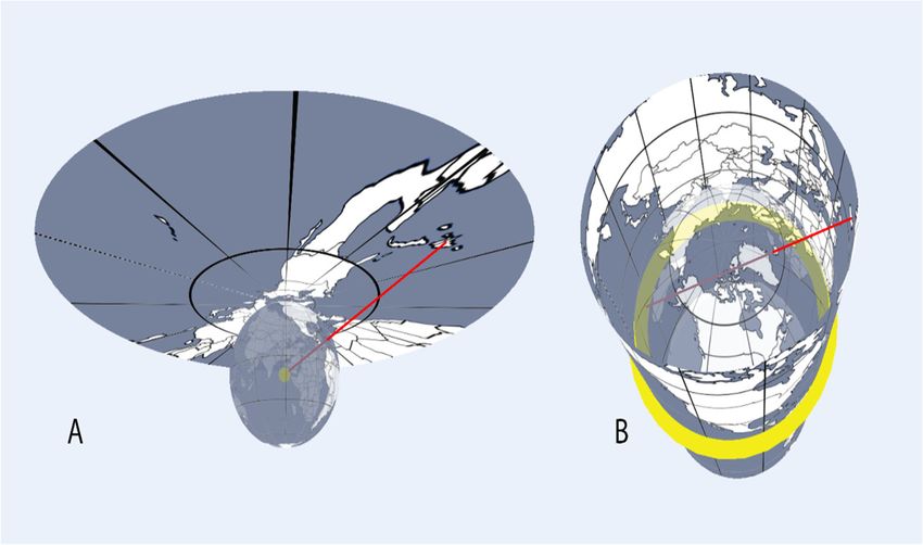
ISPRS Int. J. Geo-Inf. 2019, 8, 162                                                                         3 of 10

education platform Geographic Information Technology Training Alliance (GITTA) to make it easily
available to a wide range of learners. GITTA is accessible at http://www.gitta.info/.

2. Concept
      Providing an integrated experience for the construction process of map projections led to three
requirements. Firstly, each construction step should be easily traceable and, hence, improve the
intellectual comprehension of the entire process. Secondly, it should be possible to manually change
the parameters of each construction step to foster the understanding of the consequences that these
changes may have on the final map. Thirdly, the user should optionally be guided through each
construction step by providing tailored parameterizations for common map projections or interesting
configurations. This is advantageous since allowing an unguided exploration of parameters bears the
risk that meaningful configurations may be difficult to find. These requirements necessitate a highly
interactive application that not only allows changing each parameter in real-time, but also requires
continuously depicting the transition between two configurations such as unrolling the map, scaling
it, or setting parameters to default values. The basic objects that comprise the light source metaphor
remain the same as depicted in Figure 2.

      Figure 2. An interactive visualization following the light source metaphor to construct a map
      projection. The yellow sphere represents the point light source as the projection center. Illustrated is
      an example projection line, intersecting the globe in Cyprus and “drawing” the respective color on
      the projection surface (a disc).

     The high-level steps of the construction process and the transitions between them are depicted
in Figure 3. In the first, initial state (“rolled”), the basic projection properties such as the type of
surface and the position of the light source are defined. This already allows creating a limited set of
possible plane-based projections, such as the stereographic azimuthal or the gnomonic azimuthal
projections. Cylinder- and cone-based projections, however, need to be flattened to form the actual
map. There are numerous projections that can be obtained this way, such as Lambert’s equal area
projection or Braun’s stereographic projection. However, many projections cannot be obtained this
way such as the Mercator projection, which requires a non-linear scaling. A scaled map cannot be
directly rolled again as the introduced distortions may not be geometrically reconstructed. Therefore,
the scaling operation needs to be undone to obtain a rollable map.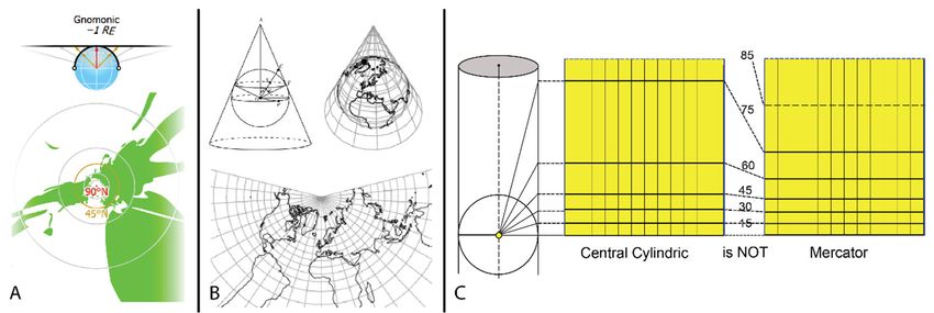
ISPRS Int. J. Geo-Inf. 2019, 8, 162 4 of 10
Figure 3. Major states of the interactive visualization process to construct different map projections.
Arrows indicate transitions between the states, which are generally realized as smooth animations.
Allowing retracing the whole process of the construction step in a continuous manner makes it
necessary to use a single three-dimensional (3D) view, in which the three main objects (globe, light
source, and projection surface) are displayed (Figure 2). Any parameter change has a direct impact
on at least one object displayed in this 3D view.
3. Projection Surface
Using a single 3D view to visualize the whole construction process has specific implications for
the projection surface as it undergoes several geometrical transformations until the final map is
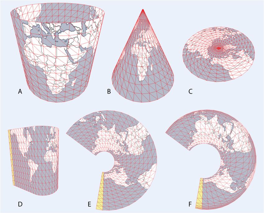
obtained (Figure 4). A single mesh is used to form all projection surfaces. Initially, this mesh structure
is constructed in the form of a cylinder based on quads with each quad consisting of two triangles
(Figure 4A). By reducing one of the two cylinder radii, a (frustum of a) cone can be constructed
(Figure 4B); by subsequently reducing the cylinder axis length, a flat disc is constructed representing
the plane (Figure 4C).
Unrolling is achieved by separating the mesh into a sequence of stripes, where each stripe
consists of a set of stacked quads. In Figure 4D, the first stripe is highlighted in yellow. All subsequent
stripes are iteratively rotated until they reside in the plane defined by the first stripe. For the second
stripe, this is done as follows: firstly, the angle and the axis of rotation need to be found. The axis of
rotation is defined by the common edge between the first and the second stripe. The angle by which
each stripe is to be rotated is equal to the angle between the normals of the two stripes. The rotation
is then applied to the second stripe and all subsequent stripes. As a consequence, the second stripe
lies in the reference plane, while all following stripes are rotated toward the reference plane (but are
not there yet). When the process is repeated for the third stripe, it will end up in the reference plane,
while all remaining stripes will be somewhat closer to it. The process is repeated until all stripes
reside in the reference plane. An intermediate result of this process for a cylinder is displayed in
Figure 4D. The ultimate result exemplified for a cone is displayed in Figure 4E.
Once flattened, the mesh can be scaled to obtain specific properties. Scaling is realized by using
a function that maps each vertex position to a new position along the vertical axis the vertex belongs
to. In the examples given in Figure 4, the vertical axes coincide with the meridians. The scaling
function can be either provided explicitly to create a desired map projection or can be defined
manually, e.g., using splines. A scaled variant of a flattened cone is depicted in Figure 4F.
This way of moving vertices to new positions in order to obtain a desired map projection based
on scaling a given map projection only yields an approximation. In fact, the image at the moved
vertex positions will be mapped exactly, while positions between vertices will be slightly inaccurate
due to interpolation. It is, therefore, important to construct a mesh with a high number of vertices to
minimize inaccurate mappings. In practice, 50 quads per stripe proved to be sufficient to reduce these
deviations to a negligible level. In addition, we want to emphasize that this way of scaling is not
trivial as the underlying formulas may make use of complicated trigonometric functions, which
cannot be easily reconstructed by simple geometric means.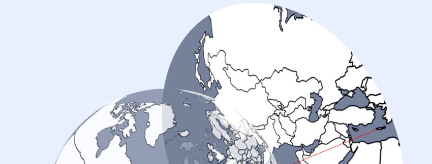
ISPRS Int. J. Geo-Inf. 2019, 8, 162                                                                         5 of 10

      Figure 4. Different ways of how the mesh is modified to represent different states of the projection
      surface: (A) a cylinder; (B) a cone; (C) a plane (disc); (D) an intermediate state during a flattening
      process; (E) a flattened cone; (F) a scaled flattened cone. The reference stripe is indicated in yellow.
      For readability, a mesh with a low resolution is depicted (30 radial and 10 vertical segments). To
      reduce graphical artefacts, a mesh with a higher resolution is recommended (e.g., 100 radial and 50
      vertical segments).

4. Light Source
     The projection center is the second dynamic object when constructing projections following the
light source metaphor. The simplest shape of a light source is that of a point, in which case, light is
emitted equally in all directions. This configuration is required for many simple map projections such
as the stereographic and gnomonic azimuthal or the central cylindrical and central conical
projections. It can be simply visualized as a glowing sphere (Figure 5A). Other projections may
require different shapes of the light source. The orthographic azimuthal projection, as a simple
example, assumes that the projection is carried out orthogonally on the plane. There are several
possibilities to visualize this arrangement, for example, by modeling the light source as a glowing
plane. However, a simpler solution is to place the point light source infinitely distant from the
projection surface, which yields parallel rays of light. Projection lines (red lines in Figure 5) can be
added to help indicate how a specific point on the projection surface obtains its color (In the
application, projection lines can be added by pressing shift and then left-clicking on the globe).

      Figure 5. Two configurations of the light source: (A) point light source placed in the center of the
      globe; (B) circular light source representing multiple varying positions of the light source depending
      on the longitude. The light rays used to draw specific points on the projection surface are highlighted
      in red.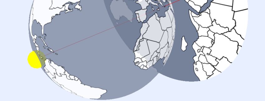
ISPRS Int. J. Geo-Inf. 2019, 8, 162                                                                 6 of 10

      There is a set of map projections which cannot be realized by a simple point light source model.
For example, the construction of Braun’s stereographic cylindrical projection assumes light rays
originating from a circular ring and passing the globe’s surface before being cast onto the projection
plane. Another special case with respect to the light source is Lambert’s cylindrical equal-area
projection which requires light rays laying in parallel planes. This corresponds to a bar-shaped light
source.
      A consequence would be that the basic light bulb metaphor can no longer be retained. In order
to cover all abovementioned cases, a light source needs to be of type (a) a point, (b) a straight line, (c)
a circular line, and (d) a circular area. The latter type enables a parallel light source without the need
to place a point light source at infinity.
      Conceptually, the introduction of different types of light sources undermines the neat light bulb
metaphor. What is missing is a single versatile light source, analogous to the projection plane whose
basic mesh construction enables forming planar, conical and cylindrical shapes. A candidate shape
for such a light source would be a scalable torus. Its parameters, the radius from the shape’s center
to the center line of the tube and the radius of the tube itself along with the scaling, enable creating
all shapes such as spheres, discs, bars, and tori.

5. Rendering
     Correctly rendering features of the earth’s surface on the projection surface requires adapting
the 3D real-time rendering pipeline as supported by common 3D application programming interfaces
(APIs) such as OpenGL/WebGL or Direct3D. The output of each rendering operation is the set of
pixels that are to be depicted on the computer screen. Hence, to accurately determine the color of a
pixel that covers the projection surface requires the following steps:
1.    Determine the pixel’s location in 3D space as if the projection surface was in the “rolled” state.
2.    Construct a projection line between the pixel’s 3D location and the light source’s 3D location.
3.    Compute the intersection with the globe.
4.    Determine the color of the globe at the intersection point (if there is any).
5.    Assign the determined color to the respective pixel on the screen.
      A more detailed explanation of these steps is given below. Changing the mesh of the projection
surface is carried out either by modifying the local position vertices vl of these triangles (e.g., by
reducing one of the radii) or by modifying the mesh’s linear transformation matrix (e.g., by changing
the orientation of the surface). The latter is typically referred to as the model matrix MM and is used
to transform the vl with respect to the local coordinates of the projection surface into global position
vertices vg with respect to the center of the 3D scene. In the next step, the so-called view matrix MV is
used to transform the vg into the view coordinates vv with respect to the position of the 3D camera
pointing to the scene. Afterward, the projection matrix Mp is used to carry out the perspective
distortion of the vv into the perspectively distorted vertices vp. The transformed triangles consisting
of vp are finally rasterized according to a given resolution, typically that of the screen. The result of
this process is the two-dimensional (2D) image I, which is shown to the user. Generally, image I can
contain pixels of other objects as well. For the sake of simplicity, we assume that it only contains
pixels that originate from the projection surface.
      As explained above, it is required to construct a line (or arcs, in some cases) between the
projection center and a point on the projection surface. The color of the point on the projection surface
is then equal to the color of the globe where it is intersected by the line. In the continuous case, there
is an infinite number of points for which these colors have to be determined. However, since I is
discrete (the screen pixels), it suffices to carry out the projection process for each of these pixels.
      This requires providing each pixel with its global position vg, which can be stored as an
additional attribute for each triangle vertex. By default, each of these attributes is interpolated during
rasterization and, thus, can be accessed when calculating the color of each pixel in I.
      The straight projection line can be constructed given vg and the projection center c. To calculate
the intersection between the line and the globe (modeled as a sphere), the equation provided by
ISPRS Int. J. Geo-Inf. 2019, 8, 162 7 of 10
Reference [9] is used. In the case of two intersections, the position closest to the projection surface is
chosen; in the case of no intersection, the pixel is colored gray.
Determining the pixel color based on the position of the intersection is carried out by sampling
a texture, i.e., an image that can be referenced using the 2D normalized coordinates u, v ∈ [0, 1].
Probably the simplest way to retrieve such normalized coordinates based on an intersection point is
as follows: firstly, the 3D coordinates with x, y, z ∈ [−1, 1] of the intersection point have to be
converted into 3D spherical coordinates with inclination θ ∈ [0, π], azimuth φ ∈ [−π, π], and radius
r = 1. Normalizing both, θ and φ, to the range [0, 1] yields an exact mapping to the required texture
coordinates u, v. This direct mapping of spherical coordinates to Cartesian coordinates requires the
texture to depict the earth in the equirectangular projection. Sampling is carried out using anisotropic
filtering to ensure a crisp image (see, e.g., Reference [10] for more details). A texture can contain any
information of interest, such as the globe’s topography, the geographic grid, or Tissot’s indicatrices.
Overlaying different textures can be achieved by blending the colors from each texture sample.
Flattening and scaling the projection surface effectively changes the global vertex positions and,
hence, the projection procedure using vl will lead to undesirable results. Therefore, before flattening
the surface, the local coordinates vl are saved as an auxiliary attribute vlr, which consequently remains
unchanged when the surface is flattened and scaled. The calculation of the intersection point is then
carried out using vgr, which is calculated by applying MM on vlr. Since vgr is known in all states, it is
possible to investigate the effects of a modified light source even if the surface is already flattened or
scaled.
6. Prototype
The proposed visualization concept was implemented in a prototypical educational tool to allow
unguided and guided exploration of the map construction process in a comprehensive and
interactive manner. Its central 3D view shows the arrangement of the required objects: the projection
surface, the light source, and the globe. Figure 6 shows the prototype in the final “scaled” state. This
state was constructed by first creating the central cylindrical projection in the “rolled” state, then
unrolling the surface to obtain the “flattened” state, and finally by manually scaling the flattened
surface to approximate the Mercator projection, representing the “scaled” state.
Figure 6. The prototype allowing for an interactive understanding on the construction of map
projections. A flattened central cylindrical projection was manually scaled in such a way that the
Mercator projection could be approximated. Tissot’s indicatrices were added to visualize the
conformity property. Left: user interface elements to explore different configurations of map
projections. Center: the three-dimensional (3D) view containing the relevant 3D objects to construct
map projections. Right: example page of the tutorial with explanations on the Mercator projection.
On the left side, a control panel allows changing the configuration in the 3D view and toggling
the transition from one state (see Figure 3) to another. The initial state is “rolled”. The availableISPRS Int. J. Geo-Inf. 2019, 8, 162 8 of 10
options during this state primarily consist of controls to modify the shape of the projection surface
(“geometry”) and to change its orientation in respect to the globe (“orientation”), as well as buttons
to create the default gnomonic azimuthal projection by pushing the “reset” button and to remove
projection lines using the “remove line” button. To trigger the transformation state, the “flatten”
button will result in an animated flattening. At the end of this animation, the state “flattened” is
obtained. The button formerly labeled “flatten” will change to “roll”, allowing to move back from the
“flattened” state to the “rolled” state. The “scaled” state can be obtained by pushing the “start
editing” button, which allows manually scaling the flat map using Bézier curves. More Bézier curves
can be added by left-clicking into the widget. They can be removed by right-clicking them. Returning
to the “flattened” state requires resetting any applied scaling using the “reset” button below the
scaling widget.
For all states, the “light source” and “layers” controls are available as their changes can be
directly propagated through all states without any limitations. It is, however, advisable to use them
primarily in the “rolled” state as this gives a better visual impression on their effects.
These controls provide high flexibility in exploring different map projections. Guided
exploration is supported via the tutorial on the right side of the application. The textual explanations
are complemented with buttons that dynamically adapt the control options on the left (and, thus, the
objects in the 3D view) to showcase important aspects. These buttons are enabled/disabled according
to the state in which they actually make sense. For example, scaling to the Mercator projection only
makes sense when the application is in the “flattened” or “scaled” state. As such it is disabled in the
“rolled” state. Additionally, a (non-comprehensive) list of map projections is provided in the tutorial,
which allows automatically creating the respective arrangements of the light source and the
projection surface.
The prototype was implemented using common web technologies HTML, CSS, JavaScript and
the libraries three.js for the 3D view and D3.js for the scaling widget. The rendering procedure was
implemented in GLSL.
7. Discussion
The prototype illustrates that the proposed way of constructing map projections based on a real-
time implementation of the light source metaphor is feasible and, as such, complements the more
conventional approach of existing libraries based on tailored formulas. Although it is believed that
this approach can bring great benefits specifically in high-school and academic undergraduate
teaching, quantitative evidence for this assumption is still missing and would require a thorough
study. The number of different parameters that need to be adapted to obtain a specific map projection
can be overwhelming and might even increase if more map projections should be supported. Hence,
it might be necessary to simplify the user interface to make it more approachable, especially for
younger students. At the time of writing, a first basic version simplifying the user interface is
available at https://gevian.github.io/GITTA-MP/basic.html.
Another limitation is the number of supported features. For example, some popular map
projections require projection arcs rather than projection lines (e.g., Plate Carrée or Lambert’s
azimuthal equal area projection). The scaling is limited to the vertical stripe axis. Some interesting
map projections (such as those of the pseudo-cylindrical family) require more complex scaling
operations. Both features require some effort to be implemented, but are considered worthy
additions, especially to support projections such as the novel Equal Earth projection [11]. Relatively
exotic map projections (e.g., Myriahedral [12]) have specific requirements such as multiple
interruptions, which would require more advanced mesh manipulation instruments. Yet, the
rendering mechanism can be applied to arbitrary geometrical surfaces, which should make the
integration of such projections feasible.
One fundamental advantage of the proposed solution is the possibility to explore different
configurations of the light source and the projection surface, as well as subsequently applying scaling
functions. This allows interactively investigating uncommon configurations and, thus, potentially
discovering entirely new map projections. A major caveat of this approach lies in the issue that theISPRS Int. J. Geo-Inf. 2019, 8, 162 9 of 10
underlying formulas (and, thus, the distortion properties) cannot be directly provided by the
application. Rather, the user would need to reconstruct the projection formulas based on the
visualization and settings as there is currently no mechanism that automatically derives the analytical
projection formulas.
When able to arbitrarily shape light sources, the question arises if light sources can be formed in
such a way as to avoid a final scaling step. This question cannot be answered right away and needs
further investigation; however, being able to show as many projections as possible using the light
source metaphor would further underline the usefulness of this interactive map projection instruction
tool.
8. Conclusions
Allowing interactively constructing map projections in a 3D environment as provided by the
described projection tool goes beyond the common static approaches provided by conventional
educational resources. As such, it is believed that it can contribute to the understanding of map
projections, especially for undergraduate and high-school students. In addition, it can bring benefits
to cartography experts as it allows an easy way to recapitulate common map projections and to
investigate uncommon configurations, eventually leading to the discovery of new map projections.
Several limitations (e.g., uniaxial scaling, no projection arcs) currently restrict the number of
constructible map projections supported by the described prototype. It is aimed to gradually address
these limitations to include the majority of common map projections and, thus, to provide a
comprehensive demonstration tool that is freely and easily accessible to a wide range of academic
institutions.
Author Contributions: Author Contributions: For research articles with several authors, a short paragraph
specifying their individual contributions must be provided. Conceptualization, Magnus Heitzler, Hans-Rudolf
Bär and Roland Schenkel; methodology, Magnus Heitzler and Hans-Rudolf Bär; software, Magnus Heitzler;
writing—Original draft, Magnus Heitzler and Hans-Rudolf Bär; writing—Review and editing, Magnus Heitzler,
Hans-Rudolf Bär, Roland Schenkel and Lorenz Hurni.
Funding: The project received funding from the GITTA association.
Conflicts of Interest: Page: 9
The authors declare no conflict of interest.
References
1. Flater, D. Understanding Geodesic Buffering—Correctly use the Buffer tool in ArcGIS. 2019. Available
online: https://www.esri.com/news/arcuser/0111/geodesic.html (accessed on 27 February 2019).
2. Aisch, G. Kartograph. 2018. Available online: https://kartograph.org/ (accessed on 27 August 2018).
3. Bostock, M.; Ogievetsky, V.; Heer, J. D3 Data-Driven Documents. IEEE Trans. Vis. Comput. Graph. 2011, 17,
2301–2309.
4. Jenny, B.; Patterson, T.; Hurni, L. Flex Projector—Interactive Software for Designing World Map
Projections. Cartograph. Perspect. 2008, 59, 12–27.
5. Kippers, R. Map Projections. 2019. Available online: https://kartoweb.itc.nl/geometrics/Map
projections/body.htm (accessed on 27 February 2019).
6. Wiki.GIS.com – The GIS Encyclopedia contributors. Map Projection. 2019.
http://wiki.gis.com/wiki/index.php/Map_projection (accessed on 27 February 2019).
7. Iliffe, J.; Lott, R. Datums and Map Projections: For Remote Sensing, GIS and Surveying; Whittles Publishing:
Dunbeath, UK, 2008.
8. Fenna, D. Cartographic Science—A Compendium of Map Projections, with Distortions; CRC Press/Taylor &
Francis Group: Boca Raton, FL, USA; London, UK; NewYork, NY, USA, 2007.
9. Eberly, D.H. 3D Game Engine Design: A Practical Approach to Real-Time Computer Graphics, 2nd ed.; Morgan
Kaufman/Elsevier: Amsterdam, NL; Boston MA, USA; Heidelberg, DE; London, UK; New York, NY, USA;
Oxford, UK; Paris, FR; San Diego, CA, USA; San Francisco, CA, USA; Singapore, SG; Sydney, AU; Tokyo,
JP; 2007.ISPRS Int. J. Geo-Inf. 2019, 8, 162 10 of 10
10. Akenine-Möller, T.; Haines, E.; Hoffman, N. Real-Time Rendering, 3rd ed.; AK Peters, Ltd.: Wellesley, MA,
USA, 2008.
11. Šavrič, B.; Patterson, T.; Jenny, B. The Equal Earth map projection. Int. J. Geogr. Inf. Sci. 2018, 33, 1–12.
12. Van Wijk, J. Unfolding the Earth: Myriahedral Projections. Cartogr. J. 2008, 45, 22–42.
.
© 2019 by the authors. Licensee MDPI, Basel, Switzerland. This article is an open access
article distributed under the terms and conditions of the Creative Commons Attribution
(CC BY) license (http://creativecommons.org/licenses/by/4.0/).You can also read