Multi-Level Surface Maps for Outdoor Terrain Mapping and Loop Closing
←
→
Page content transcription
If your browser does not render page correctly, please read the page content below
Multi-Level Surface Maps for Outdoor Terrain
Mapping and Loop Closing
Rudolph Triebel Patrick Pfaff Wolfram Burgard
University of Freiburg
Georges-Koehler-Allee 79, 79110 Freiburg, Germany
{triebel,pfaff,burgard}@informatik.uni-freiburg.de
Abstract— To operate outdoors or on non-flat surfaces, mobile maps (MLS maps) offer the opportunity to model environ-
robots need appropriate data structures that provide a compact ments with more than one traversable level. Whereas the
representation of the environment and at the same time support knowledge about horizontal surfaces is well suited to support
important tasks such as path planning and localization. One
such representation that has been frequently used in the past traversability analysis and path planning, it provides only
are elevation maps which store in each cell of a discrete grid weak support for localization of the vehicle or registration
the height of the surface in the corresponding area. Whereas of different maps. Modeling only the surfaces means that
elevation maps provide a compact representation, they lack the vertical structures, which are frequently perceived by ground
ability to represent vertical structures or even multiple levels. based vehicles cannot be used to support localization and
In this paper, we propose a new representation denoted as
multi-level surface maps (MLS maps). Our approach allows to registration. To avoid this problem, our MLS maps additionally
store multiple surfaces in each cell of the grid. This enables a represent intervals corresponding to vertical objects in the
mobile robot to model environments with structures like bridges, environment. The advantage of this approach is that they can
underpasses, buildings or mines. Additionally, they allow to be compactly stored and at the same time can be used as
represent vertical structures. Throughout this paper we present features that support the data association problem during the
algorithms for updating these maps based on sensory input, to
match maps calculated from two different scans, and to solve the alignment of maps.
loop-closing problem given such maps. Experiments carried out
with a real robot in an outdoor environment demonstrate that
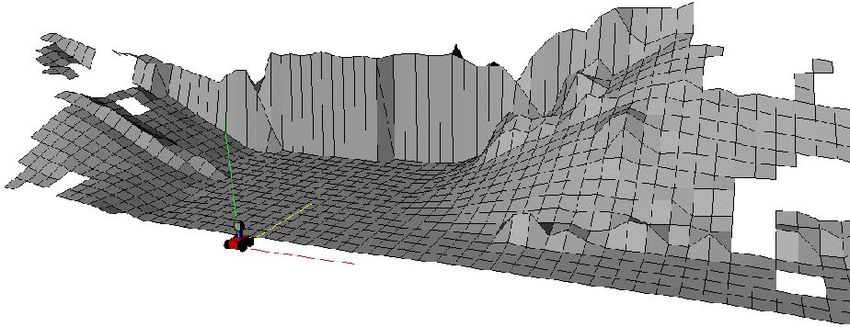
our approach is well-suited for representing large-scale outdoor As a motivating example, consider the three-dimensional
environments. data points shown in Figure 1(a). They have been acquired
with a mobile robot standing in front of a bridge. The resulting
I. I elevation map, which is computed from averaging over all scan
points that fall into a cell of a horizontal grid (given a vertical
The problem of learning maps with mobile robots has
projection), is depicted in Figure 1(b). As can be seen from
been intensively studied in the past. Especially in situations,
the figure, the underpass has completely disappeared and the
in which robots are deployed outdoors or in environments
elevation map shows a non-traversable object. Additionally,
with non-flat surfaces, the ability to traverse specific areas
when the environment contains vertical structures, we typically
of interest needs to be known accurately. In this context,
obtain varying average height values depending on how much
geometric representations have become popular. However, full
of this vertical structure is contained in a scan. When two
three-dimensional models typically have high computational
such elevation maps need to be aligned, such errors can lead
demands that prevent them from being directly applicable in
to imperfect registrations. The corresponding map calculated
large-scale environment.
with the approach of Pfaff et al. [20], which allows to deal
One popular approach to overcome this problem are eleva-
with vertical and overhanging objects, is shown in Figure 1(c).
tion maps, which apply a 2 21 -dimensional representation. An
Obviously, this approach correctly represents the underpass
elevation map consists of a two-dimensional grid in which
and allows the robot to move through the tunnel, but it makes
each cell stores the height of the territory. Whereas this
it impossible to travel over the bridge. The corresponding
approach leads to a substantial reduction of the memory
MLS map is shown in Figure 1(d). As can be seen, this
requirements, it can be problematic when a robot has to utilize
representation can correctly represent the individual surfaces.
these maps for navigation or when it has to register two
It also shows that vertical structures are correctly represented.
different maps in order to integrate them. Even extensions of
elevation maps that allow to handle vertical or overhanging
objects [20] can only be applied to environments with single This paper is organized as follows. After discussing of
surfaces. For example, a robot that uses extended elevation related work in the following section, we will describe our
maps cannot plan a path under and at the same time over a approach of MLS maps in Section III. Section IV then
bridge. introduce our constraint-based pose estimation procedure for
In this paper, we propose an extension of elevation maps calculating consistent maps. Finally, we present experimental
towards multiple surfaces. These so-called multi-level surface results in Section V.Fig. 1. Scan (point set) of a bridge (a), standard elevation map computed from this data set (b), extended elevation map which correctly represents the
underpass under the bridge (c), and multi level surface map that correctly represents the height of the vertical objects (d)
II. R W is limited.
In order to avoid the complexity of full three-dimensional
The problem of learning three-dimensional representations maps, several researchers have considered elevation maps as
has been studied intensively in the past. Recently, several an attractive alternative. The key idea underlying elevation
techniques for acquiring three-dimensional data with 2d range maps is to store the 2 21 -dimensional height information of
scanners installed on a mobile robot have been developed. A the terrain in a two-dimensional grid. Bares et al. [2] as
popular approach is to use multiple scanners that point towards well as Hebert et al. [8] use elevation maps to represent the
different directions [7], [25], [26]. An alternative is to use environment of a legged robot. They extract points with high
pan/tilt devices that sweep the range scanner in an oscillating surface curvatures and match these features to align maps
way [15], [22]. More recently, techniques for rotating 2d range constructed from consecutive range scans. Parra et al. [21]
scanners have been developed [10], [30]. represent the ground floor by elevation maps and use stereo
Many authors have studied the acquisition of three- vision to detect and track objects on the floor. Singh and
dimensional maps from vehicles that are assumed to operate Kelly [24] extract elevation maps from laser range data and
on a flat surface. For example, Thrun et al. [25] present an use these maps for navigating an all-terrain vehicle. Ye and
approach that employs two 2d range scanners for constructing Borenstein [31] propose an algorithm to acquire elevation
volumetric maps. Whereas the first is oriented horizontally maps with a moving vehicle carrying a tilted laser range
and is used for localization, the second points towards the scanner. They propose special filtering algorithms to eliminate
ceiling and is applied for acquiring 3d point clouds. Früh and measurement errors or noise resulting from the scanner and the
Zakhor [5] apply a similar idea to the problem of learning motions of the vehicle. Lacroix et al. [11] extract elevation
large-scale models of outdoor environments. Their approach maps from stereo images. Hygounenc et al. [9] construct
combines laser, vision, and aerial images. Furthermore, several elevation maps with an autonomous blimp using 3d stereo
authors have considered the problem of simultaneous mapping vision. They propose an algorithm to track landmarks and to
and localization (SLAM) in an outdoor environment [4], [6], match local elevation maps using these landmarks. Olson [18]
[27]. These techniques extract landmarks from range data and describes a probabilistic localization algorithm for a planetary
calculate the map as well as the pose of the vehicles based on rover that uses elevation maps for terrain modeling. In this
these landmarks. Our approach described in this paper does paper, we present MLS maps, which can be regarded as an
not rely on the assumption that the surface is flat. It uses m extension to elevation maps. Our approach allows to compactly
MLS maps to capture the three-dimensional structure of the represent multiple surfaces in the environment as well as
environment and is able to estimate the pose of the robot in vertical structures. This allow a mobile robot to correctly
all six degrees of freedom. deal with multiple traversable surfaces in the environment
One of the most popular representations are raw data points as they, for example, occur in the context of bridges. Our
or triangle meshes [1], [12], [22], [28]. Whereas these models approach also represents an extension of the work by Pfaff et
are highly accurate and can easily be textured, their disad- al. [20]. Whereas this approach allows to deal with vertical
vantage lies in the huge memory requirement, which grows and overhanging objects in elevation maps, it lacks the ability
linearly in the number of scans taken. Accordingly, several to represent multiple surfaces.
authors have studied techniques for simplifying point clouds Recently, several authors have studied the problem of si-
by piecewise linear approximations. For example, Hähnel et multaneous localization and mapping in the context of mobile
al. [7] use a region growing technique to identify planes. robots operating on a non-flat surface. For example, Davison
Liu et al. [13] as well as Martin and Thrun [14] apply the et al. [3] presented an approach to vision based SLAM with
EM algorithm to cluster range scans into planes. Recently, a single camera moving freely through the environment. This
Triebel et al. [29] proposed a hierarchical version that takes approach uses an extended Kalman Filter to simultaneously
into account the parallelism of the planes during the clus- update the pose of the camera and the 3d feature points
tering procedure. An alternative is to use three-dimensional extracted from the camera images. More recently, Nüchter et
grids [16] or tree-based representations [23], which only grow al. [17] developed a mobile robot that builds accurate three-
linearly in the size of the environment. According to the non- dimensional models with a mobile robot. In this approach, loop
planar structure of natural outdoor environments and the space closing is achieved by uniformly distributing the estimated
requirements for large-scale environments, the applicability of odometry error over the poses in a loop. In contrast, the work
these representations and approximations in such environments described here employs MLS maps and globally optimizes theµ a) Map Creation: An MLS map can be generated in two
different ways: either from a set of 3D measurements, i.e. a
σ
point cloud with variances, or by joining two other MLS maps
Z into one. Both ways are equivalent, i.e. if map m1 is created
d
from point cloud C1 and map m2 from cloud C2 , then the
map m3 that results from joining m1 and m2 is identical to the
map generated by the joined point cloud C3 = C1 ∪ C2 . For a
given point cloud C with variances σ1 , . . . , σn the MLS map
is created as follows:
• Each map cell with index (i, j) collects all points p =
X (x, y, z), s.t. si ≤ x ≤ s(i + 1) and s j ≤ y ≤ s( j + 1) where
Fig. 2. Example of different cells in an MLS Map. Cells can have many s denotes the size (edge length) of a map cell.
surface patches (cell A), represented by the mean and the variance of the • In each cell, we calculate a set of height intervals from
measured height. Each surface patch can have a depth, like the patch in cell the height values of the stored points. As long as two
B. Flat objects are represented by patches with depth 0, as shown by the patch
in cell C. consecutive height values are closer than a given gap size
γ, they belong to the same interval. This means that two
intervals are at least γ meters away from each other. The
pose estimates for calculating consistent maps. To achieve this, gap size should be chosen so that a robot that navigates
we efficiently solve the data association problem that occurs, through the map can still pass the gap, i.e., it should be
when two maps with different estimates about the surface higher than the robot height. In our implementation we
levels have to be matched or combined. choose 1.0m.
III. M L S M • The intervals are classified as a horizontal or a vertical
structure. These structures are distinguished according to
Suppose we are given a set of N 3D scan points C = the height of the interval. If it exceeds a thickness value
{p1 , . . . , pN } with pi ∈ 3 , and a set of variances {σ21 , . . . , σ2N }. τ = 10cm, it is considered as vertical, otherwise it is
Here, the variance σ2i expresses the uncertainty in the range horizontal.
measurement from which point pi was computed. This uncer- • For each interval classified as vertical, we store the mean
tainty grows with the measured distance. In the following, we and variance of the highest measurement in the interval.
assume that the uncertainty is equal in all three dimensions, The intuition behind this is that for traversability only
in particular the variance in height is assumed to be identical the highest measurement is relevant. Additionally, we
to σ2i . Although this assumption is often violated in real store the length of the interval, which is identified with
environments, this approximation turned out to be viable for the depth d mentioned above. This value is used when
our applications. Regarding this, we define a measurement z matching two MLS maps together.
as a pair (p, σ2 ) of a 3D point and a variance. • For each horizontal object in a cell, we compute a mean
A. Map Representation µ and a variance σ from all measurements in the interval.
A multi-level surface map (MLS map) consists of a 2D grid This is done by applying the Kalman update rule to all
of variable size where each cell ci j , i, j ∈ in the grid stores measurements. The depth d of a horizontal object is set
a list of surface patches P1i j , . . . , PiKj . A surface patch in this to 0.
context is represented as the mean µkij and variance σkij of the After computing the means, variances and depths of the
measured heights at the position of the cell ci j in the map. Each surface patches, we delete the point cloud data. All further
surface patch in a cell reflects the possibility of traversing the calculations are performed only on the map data. This substan-
3D environment at the height given by the mean µkij , while the tially reduces the memory required for an MLS map compared
uncertainty of this height is represented by the variance σkij . to point clouds and at the same time achieves a highly accurate
Throughout this paper, we assume that the error in the height representation.
underlies a Gaussian distribution, therefore we will use the b) Map Update: Whenever a new measurement z =
terms surface patch and Gaussian in a cell interchangeably. (p, σ) is inserted into an MLS map, we first need to know
In addition to the mean and variance of a surface patch, whether the measurement belongs to an object that is already
we also store a depth value d for each patch. This depth value represented in the map, or if it corresponds to a new object. To
reflects the fact that a surface patch can be on top of a vertical this end, we first determine the cell ci j in which the measured
object like a building, bridge or ramp. In these cases, the depth point falls. Then we find the Gaussian (µkij , σkij ) in ci j whose
is defined by the difference of the height hkij of the surface mean µkij is closest to the height of z. If this Gaussian is close
patch and the height h′i j k of the lowest measurement that is enough, we update it with the new measurement z, again using
considered to belong to the vertical object. For flat objects the Kalman update rule. In our implementation, we define a
like the floor, the depth is 0. Figure 2 depicts some examples Gaussian to be close to a measurement z if the height value
of the map cells in an MLS map. of z is within 3σ of the Gaussian.the error function e is defined by the sum of squared Maha-
lanobis distances between the points xic and the transformed
point y jc . In the following, we denote this Mahalanobis dis-
tance as d(xic , y jc ).
In principle, one could define this function to directly
operate on the Gaussians when aligning two different MLS
maps. One disadvantage of this approach, however, is that
a MLS map of one single scan typically includes a huge
Fig. 3. Classification result for the MLS map depicted in Figure 1(d). The number of Gaussians (15,318 on average in the data sets shown
three colors/grey levels indicate the classification result for the individual
surface patches into traversable, non-traversable, and vertical ones. in this paper). Accordingly, the nearest neighbor search in
the ICP algorithm requires a lot of computational resources.
Additionally, we need to take care of the problem that the
If z is far from the nearest Gaussian, it is still possible intervals corresponding to vertical structures vary substantially
that it corresponds to a vertical object. This can be found out depending on the view-point. Moreover, the same vertical
by checking whether z is inside the occupancy of one of the structure may lead to varying heights in the surface map when
Gaussians in the cell. In this case, the measurement z is simply sensed from different points. In practical experiments, we ob-
disregarded, because a vertical object with a Gaussian on top served that this introduces serious errors and often prevents the
already exists. Otherwise, z is introduced as a new Gaussian ICP algorithm from convergence. To overcome this problem,
into the cell. we separate Equation (1) into three components each mini-
mizing the error over the individual classes of points. These
B. Traversability Analysis and Feature Extraction three terms correspond to the three individual classes, namely
In the past, it has often been reported that the data associ- surface patches corresponding to vertical objects, traversable
ation can seriously be improved by extracting features from surface patches, and non-traversable surface patches.
the data [17], [20]. In addition to the vertical structures, we Let us assume that uic and u′jc are corresponding points,
therefore additionally classify the horizontal surface patches extracted from vertical objects. The number of points sam-
according to their traversability. To determine whether a sur- pled from every interval classified as vertical depends on
face patch is traversable, we find the nearest Gaussian in each the height of this structure. In our current implementation,
neighboring cell. In our approach, a surface patch can only be we typically uniformly sample four points per meter. The
traversable if at least 5 of the 8 neighboring cells exist and if corresponding points vic and v′jc are extracted from traversable
the distance in height between the patch and all its neighbors is surface patches, wic and w′jc are extracted from not traversable
less than 10cm. Figure 3 shows the classification result for the surfaces. The resulting error function then is
MLS map depicted in Figure 1(d). The three colors/grey levels C1 C2 C3
X X X
indicate the classification result. The yellow/light grey parts e(R, t) = dv (uic , u′jc ) + d(vic , v′jc ) + d(wic , w′jc ). (2)
of the surfaces represent the traversable surface patches. The c=1 c=1 c=1
blue/dark areas are the non-traversable parts of the surfaces | {z } | {z } | {z }
vertical cells traversable non-traversable
and the red/medium grey structures represent the vertical
objects. In this equation, the distance function dv calculates the Ma-
halanobis distance between the lowest points in the particular
C. Map Matching cells. To increase the efficiency of the matching process, we
To calculate the alignments between two local MLS maps only consider a subset of these features by sub-sampling.
calculated from individual scans, we apply the ICP algorithm.
The goal of this process is to find a rotation matrix R and a IV. L C
translation vector t that minimize an appropriate error function.
Assuming that the two maps are represented by a set of The ICP-based scan matching technique described above
Gaussians, the algorithm first computes two sets of feature works well for the registration of single robot poses into one
points, X = {x1 , . . . , xN1 } and Y = {y1 , . . . , yN2 }. Then in a global reference frame. However, the individual scan matching
second step the algorithm computes a set of C index pairs or processes result in small residual errors which quickly accu-
correspondences (i1 , j1 ), . . . , (iC , jC ) such that the point xic in mulate over time and usually result in globally inconsistent
X corresponds to the point y jc in Y for c = 1, . . . , C. Then, in maps. In practice, this typically becomes apparent when the
a third step, the error function e defined by robot encounters a loop, i.e., when it returns to a previously
visited place. Especially in big loops this error grows so large
C that the resulting inconsistencies make the map useless for
1X
e(R, t) := (xi − (Ry jc + t))T Σ−1 (xic − (Ry jc + t)), (1) navigation. Accordingly, techniques for calculating globally
C c=1 c
consistent maps are necessary. In the system described here,
is minimized. Here, Σ denotes the covariance matrix of the we apply a technique similar to the one presented in [19] to
Gaussian corresponding to each pair (xi , yi ). In other words, correct for the accumulated error when closing a loop.A. Network-based Pose Optimization In other words, g contains all local constraints expressed as 3D
translation and rotation. Next we define the constraint function
Suppose the robot recorded 3D scans at N different poses
f : 6N → 6M that maps robot poses to local constraints.
P1 , . . . , PN . A pose is defined as a 6-tuple (x, y, z, ϕ, ϑ, ψ)
of location (x, y, z) and orientation (ϕ, ϑ, ψ). Whenever two ..
.
local MLS maps mi and m j corresponding to the poses Pi
f (x1 , . . . , ψ1 , . . . , xN , . . . , ψN ) := α(P−1 i P j ) (5)
and P j are matched to each other using the map matching ..
technique described above, a constraint is imposed on the .
poses Pi and P j . If we represent all these constraints as
Here we introduced the function α which converts a pose trans-
undirected links in a graph, where the nodes are defined
form P into its 6 parameters (x, y, z, ϕ, ϑ, ψ). This constraint
by the robot poses, we obtain a network of robot poses. A
function f is non-linear due to the rotations. We therefore
global pose optimization that takes all local constraints into
linearize it according to f (p) ≈ F|p + J|p ∆p where p is
account can be performed on such a pose network. In the
the vector of all robot poses and J|p is the Jacobian of the
literature, many different approaches for network-based pose
constraint function f at p. At each iteration of the pose
optimization can be found. Recently, a good overview and
optimization F|p and J|p are recomputed for the new poses and
comparison of different approaches has been presented by
we will write simply F and J for better readability. The global
Olson et al. [19]. They authors also present a new algorithm
pose optimization can then be formulated as the minimization
based on a modified stochastic gradient descent (SGD) that
of the squared error:
is fast and robust against poor initial pose estimates. For our
application, we implemented both the LU decomposition [19] argmind k Jd − r k2 (6)
and the SGD approach. Both gave good results, although the
Here we substituted ∆p by d and (F − g) by r.
LU decomposition appeared to be slightly more robust.
By deriving with respect to d and setting to zero we obtain
B. Constraints between Robot Poses J T Jd = JT r (7)
As described above, the scan matching between two local This is a standard linear algebra problem which can be solved
MLS maps mi and m j is done by minimizing the error by LU decomposition or by multiplication with the pseudo-
function e(R, t) from Equation 2. After convergence of the inverse of J T J. The overall algorithm can then be described
ICP algorithm we have a set of correspondences between the by iterating the following steps:
feature sets Fi = (Ui , Vi , Wi ) and F j = (U j , V j , W j ) where • Compute F and J from the poses p.
Ui = {ui1 , . . . , uiC1 } and U j = {u j1 , . . . , u jC1 }. The other fea- • Minimize (6) according to Equation (7).
ture subsets Vi , Wi , V j , W j are defined analogously. Given • Compute new poses: p ← p + d.
these correspondences we define a local constraint between This is repeated as long as the residual r exceeds a threshold
two robot poses Pi and P j as the rigid-body transformation or a maximum number of iterations is reached.
between features in the local reference frame at Pi and the
corresponding features in the local reference frame at P j . This D. Implementation Details
means, if the scan matcher returns a rotation matrix Ri j and In our experiments it turned out that the described pose
a translation vector ti j between the global coordinates of the optimization technique works well in cases where the number
features, our local constraint T i j is defined by of robot poses was around 70. However, the larger the loops
are the higher is the initial pose estimation error from odom-
Ti j := P−1
i (Ri j P j (fic ) + ti j ) (3) etry, and it is not enough overlap left for the scan matching
algorithm to find correspondences between the first and the
Here we use the notation P j (fic ) for the function that trans- last robot poses. Therefore we proceed as follows: Considering
forms a feature fic from the local reference frame at the that the local scan matches between consecutive robot poses
robot position P j to the global reference frame. Accordingly, is highly accurate, we match local maps corresponding to 5
P−1 transforms a feature in global coordinates into the local consecutive poses into new and bigger local maps. This means
reference frame at position P j . that maps m1 , . . . , m5 are matched into the new map m̄1 , maps
m6 , . . . , m10 into m̄2 and so on. This way we obtain a set
C. LU decomposition of N5 new local maps, which reduces the pose optimization
Using the above notation we can now formulate the pose problem. A further improvement can be achieved by increasing
optimization problem. For a given set of initial robot poses the overlap between consecutive local maps m̄i and m̄i+1 . This
P1 , . . . , PN the scan matcher returns a set of local constraints can be done by adding the last partial map from m̄i to m̄i+1 .
T i j for i, j = 1, . . . , N, i , j according to Equation 3. These For example, the local map m5 is then also a part of the new
constraints are then encoded in a goal vector g of length 6M local map m̄2 . In this way, the scan matching error between
where M is the number of constraints T i j . the joined local maps m̄i and m̄ j can be reduced and the
global pose optimization is more likely to converge to a global
g := (. . . , xi j , yi j , zi j , ϕi j , ϑi j , ψi j , . . .) (4) optimum.Fig. 4. Two views of the resulting MLS map of the first experiment with a cell size of 10cm x 10cm. The area scanned by the robot spans approximately
195 by 146 meters. During the data acquisition, where the robot collected 77 scans consisting of 20,207,000 data points, the robot traversed a loop with a
length of 312m.
Fig. 5. Resulting MLS map of the second experiment with a cell size of 10cm x 10cm. The area scanned by the robot spans approximately 299 by 147
meters. During the data acquisition, where the robot collected 172 scans consisting of 45,139,000 data points, the robot traversed a loop with a length of
560m.
V. E accuracy. Additionally, they show that our representation is
well-suited for global pose estimation and loop closure.
Our approach has been implemented and evaluated using
our mobile outdoor platform Herbert which is a Pioneer II AT In the first experiment we acquired 77 scans consisting of
robot equipped with a SICK LMS 291 range sensor mounted 20,207,000 data points. The area scanned by the robot spans
on an AMTEC wrist PW70. To acquire the data, we steered approximately 195 by 146 meters. During the data acquisition,
the robot over the university campus. On its path, the robot the robot traversed a loop with a length of 312m. Figure 4
encountered two loops. Additionally, it traversed over a bridge shows two views of the resulting MLS map with a cell size
and through the corresponding underpass. The goal of these of 10cm x 10cm. The yellow/light grey surface patches are
experiments is to demonstrate that our representation yields classified as traversable. It requires 57.96 MBytes to store the
a significant reduction of the memory requirements compared computed map, where 24% of 2,847,300 cells are occupied.
to a point cloud representation, while still providing sufficient In the second experiment we acquired 172 scans consistingof 45,139,000 data points. The area scanned by the robot spans [9] E. Hygounenc, I.-K. Jung, P. Souères, and S. Lacroix. The autonomous
approximately 299 by 147 meters. During the data acquisition, blimp project of laas-cnrs: Achievements in flight control and terrain
mapping. International Journal of Robotics Research, 23(4-5):473–511,
the robot traversed a loop, which has a length of 560m. 2004.
Figure 5 shows the resulting MLS map with a cell size of 10cm [10] P. Kohlhepp, M. Walther, and P. Steinhaus. Schritthaltende 3D-
x 10cm. The yellow/light grey surface patches are classified as Kartierung und Lokalisierung für mobile inspektionsroboter. In
18. Fachgespräche AMS, 2003. In German.
traversable. It requires 73.33 MBytes to store the whole map, [11] S. Lacroix, A. Mallet, D. Bonnafous, G. Bauzil, S. Fleury and; M. Herrb,
where 20% of 4,395,300 cells are occupied. and R. Chatila. Autonomous rover navigation on unknown terrains:
Functions and integration. International Journal of Robotics Research,
VI. C 21(10-11):917–942, 2002.
[12] M. Levoy, K. Pulli, B. Curless, S. Rusinkiewicz, D. Koller, L. Pereira,
In this paper, we presented multi-level surface maps as a M. Ginzton, S. Anderson, J. Davis, J. Ginsberg, J. Shade, and D. Fulk.
novel representation for outdoor environments. Compared to The digital michelangelo project: 3D scanning of large statues. In
elevation maps, multi-level surface maps (MLS maps) store Proc. SIGGRAPH, pages 131–144, 2000.
[13] Y. Liu, R. Emery, D. Chakrabarti, W. Burgard, and S. Thrun. Using
in each cell of a discrete grid a list of surfaces. Additionally, EM to learn 3D models with mobile robots. In Proceedings of the
they use intervals to represent vertical structures. We presented International Conference on Machine Learning (ICML), 2001.
algorithms for updating multi-level surface maps based on [14] C. Martin and S. Thrun. Online acquisition of compact volumetric maps
with mobile robots. In IEEE International Conference on Robotics and
sensory input, for matching such maps and for solving the Automation (ICRA), Washington, DC, 2002. ICRA.
loop-closing problem using this representation. [15] M. Montemerlo and S. Thrun. A multi-resolution pyramid for outdoor
We also described an implementation of multi-level surface robot terrain perception. In Proc. of the National Conference on Artificial
Intelligence (AAAI), 2004.
maps on a Pioneer II AT platform equipped with a laser [16] H.P. Moravec. Robot spatial perception by stereoscopic vision and 3d
range scanner mounted on a pan/tilt unit. We presented large- evidence grids. Technical Report CMU-RI-TR-96-34, Carnegie Mellon
scale maps learned from the data acquired with this robot. University, Robotics Institute, 1996.
[17] A. Nüchter, K. Lingemann, J. Hertzberg, and H. Surmann. 6d SLAM
The resulting maps show a high accuracy and at the same with approximate data association. In Proc. of the 12th Int. Conference
time require one order of magnitude less space than the on Advanced Robotics (ICAR), pages 242–249, 2005.
original point data. Additionally, the results demonstrate that [18] C.F. Olson. Probabilistic self-localization for mobile robots. IEEE
Transactions on Robotics and Automation, 16(1):55–66, 2000.
multi-level surface maps allow mobile robots to operate in [19] E. Olson, J. Leonard, and S. Teller. Fast iterative alignment of pose
environments with multiple levels. In one of our experiments graphs with poor estimates. In ICRA, 2006. to appear.
the robot successfully traveled over a bridge and through the [20] Pfaff P. and Burgard W. An efficient extension of elevation maps for
outdoor terrain mapping. In Proc. of the International Conference on
corresponding underpass. Field and Service Robotics (FSR), pages 165–176, 2005.
[21] C. Parra, R. Murrieta-Cid, M. Devy, and M. Briot. 3-d modelling and
A robot localization from visual and range data in natural scenes. In 1st
International Conference on Computer Vision Systems (ICVS), number
This work has partly been supported by the German Re- 1542 in LNCS, pages 450–468, 1999.
search Foundation (DFG) within the Research Training Group [22] K. Pervölz, A. Nüchter, H. Surmann, and J. Hertzberg. Automatic
1103 and under contract number SFB/TR-8. reconstruction of colored 3d models. In Proc. Robotik 2004, 2004.
[23] H. Samet. Applications of Spatial Data Structures. Addison-Wesley
R Publishing Inc., 1989.
[24] S. Singh and A. Kelly. Robot planning in the space of feasible actions:
[1] P. Allen, I. Stamos, A. Gueorguiev, E. Gold, and P. Blaer. Avenue: Two examples. In Proc. of the IEEE Int. Conf. on Robotics & Automation
Automated site modeling in urban environments. In Proc. of the 3rd (ICRA), 1996.
Conference on Digital Imaging and Modeling, pages 357–364, 2001. [25] S. Thrun, W. Burgard, and D. Fox. A real-time algorithm for mobile
[2] J. Bares, M. Hebert, T. Kanade, E. Krotkov, T. Mitchell, R. Simmons, robot mapping with applications to multi-robot and 3D mapping. In
and W. R. L. Whittaker. Ambler: An autonomous rover for planetary Proc. of the IEEE Int. Conf. on Robotics & Automation (ICRA), 2000.
exploration. IEEE Computer Society Press, 22(6):18–22, 1989. [26] S. Thrun, D. Hähnel, D. Ferguson, M. Montemerlo, R. Triebel, W. Bur-
[3] A.J. Davison, Y. Gonzalez Cid, and N. Kita. Real-time 3d SLAM with gard, C. Baker, Z. Omohundro, S. Thayer, and W. Whittaker. A system
wide-angle vision. In Proc. of the 5th IFAC Symposium on Intelligent for volumetric robotic mapping of abandoned mines. In Proc. of the
Autonomous Vehicles (IAV), 2004. IEEE Int. Conf. on Robotics & Automation (ICRA), 2003.
[4] G. Dissanayake, P. Newman, S. Clark, H.F. Durrant-Whyte, and [27] S. Thrun, Y. Liu, D. Koller, A.Y. Ng, Z. Ghahramani, and H. Durant-
M. Csorba. A solution to the simultaneous localisation and map building Whyte. Simultaneous localization and mapping with sparse extended
(SLAM) problem. IEEE Transactions on Robotics and Automation, information filters. International Journal of Robotics Research, 23(7-
17(3):229–241, 2001. 8):693–704, 2004.
[5] C. Früh and A. Zakhor. An automated method for large-scale, ground- [28] S. Thrun, C. Martin, Y. Liu, D. Hähnel, R. Emery Montemerlo, C. Deep-
based city model acquisition. International Journal of Computer Vision, ayan, and W. Burgard. A real-time expectation maximization algorithm
60:5–24, 2004. for acquiring multi-planar maps of indoor environments with mobile
[6] J. Guivant and E. Nebot. Optimization of the simultaneous localization robots. IEEE Transactions on Robotics and Automation, 20(3):433–442,
and map building algorithm for real time implementation. IEEE 2003.
Transactions on Robotics and Automation, 17(3):242–257, May 2001. [29] R. Triebel, F. Dellaert, and W. Burgard. Using hierarchical EM to extract
In press. planes from 3d range scans. In Proc. of the IEEE Int. Conf. on Robotics
[7] D. Hähnel, W. Burgard, and S. Thrun. Learning compact 3d models & Automation (ICRA), 2005.
of indoor and outdoor environments with a mobile robot. Robotics and [30] O. Wulf, K-A. Arras, H.I. Christensen, and B. Wagner. 2d mapping of
Autonomous Systems, 44(1):15–27, 2003. cluttered indoor environments by means of 3d perception. In ICRA-04,
[8] M. Hebert, C. Caillas, E. Krotkov, I.S. Kweon, and T. Kanade. Terrain pages 4204–4209, New Orleans, apr 2004. IEEE.
mapping for a roving planetary explorer. In Proc. of the IEEE [31] C. Ye and J. Borenstein. A new terrain mapping method for mobile
Int. Conf. on Robotics & Automation (ICRA), pages 997–1002, 1989. robot obstacle negotiation. In Proc. of the UGV Technology Conference
at the 2002 SPIE AeroSense Symposium, 1994.You can also read