Long-run impacts of early life health interventions - Center for Economic Studies (CES)

Long-run impacts of early life health
                   interventions

                   Melanie Lührmann   Royal Holloway, University of London and IFS

                   September 16, 2020

c Royal Holloway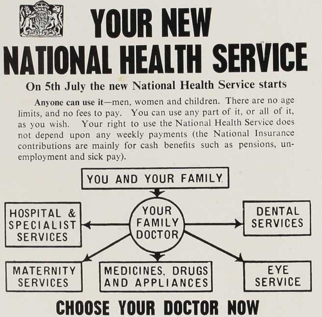

Early life interventions

    • A large literature documents large effects of early life
      environments on well-being of infants’ and children’s survival and
      childhood outcomes, and into adulthood (see Almond et al. 2019
      for a survey)
      → large returns to early investments to improve childhood
      environments
    • pareto-improvement through early targeting of redistributive
      investments?

c Royal Holloway

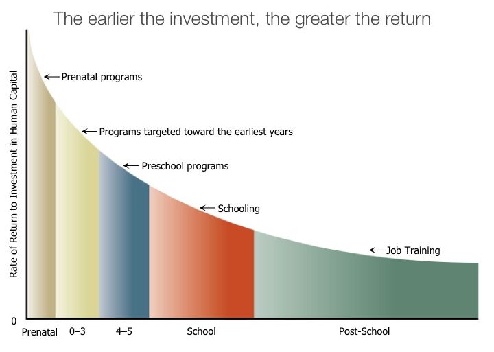
The “Heckman curve”

c Royal Holloway

Early life interventions

    • A large fraction of research focused on the role of education
      interventions and on cognitive outcomes
      → Head Start, Carolina Abecedarian Project, Perry preschool
      programs,... (see Heckman and many others)
    • in parallel, a large literature on health and nutrition conditions in
      utero establishes large returns to prenatal programs ... (e.g.
      Currie and Gruber 1996b)
      ...in terms of infancy survival
      ...education
      ...childhood health
    • emerging body of research on conditions in the infancy period
      (Bütikofer et al, 2019; Hoynes et al. 2016; Currie and Gruber
      1996a; Hjort et al. 2017; Bhalotra and Venkataramani 2015)

c Royal Holloway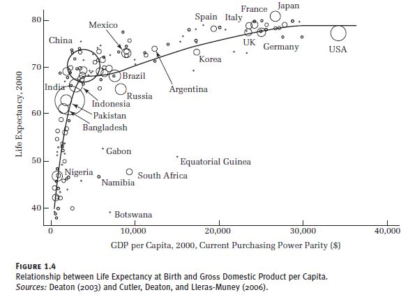

Early life interventions - types
    Type of interventions (or shocks):
    • education/cognition
      (parental time investment, stimuli, play, childcare policies,...)
    • nutrition/malnutrition
      (hunger, famine, food supplementation, school meals,
      breastfeeding, SNAP (food stamps) and similar programs)
    • healthcare/disease
            • universal healthcare or healthcare for the poor (Medicaid, NHS)
            • infectious disease outbreaks (diarrhea, tuberculosis, pandemics)
            • new drugs or treatments that improve infant and childhood
              health(e.g. deworming drugs, penicillin)

    • welfare systems (e.g. EITC, maternity leave, conditional cash
      transfers)
    • pollution/sanitation/weather
c Royal Holloway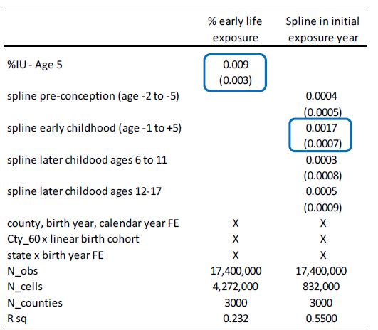

Early life interventions - stage by stage

    Fast growing literature on the (contemporaneous and long-run)
    impact of interventions and shocks
    • in utero
    • during infancy (i.e. in the first year of life)
    • during preschool years

c Royal Holloway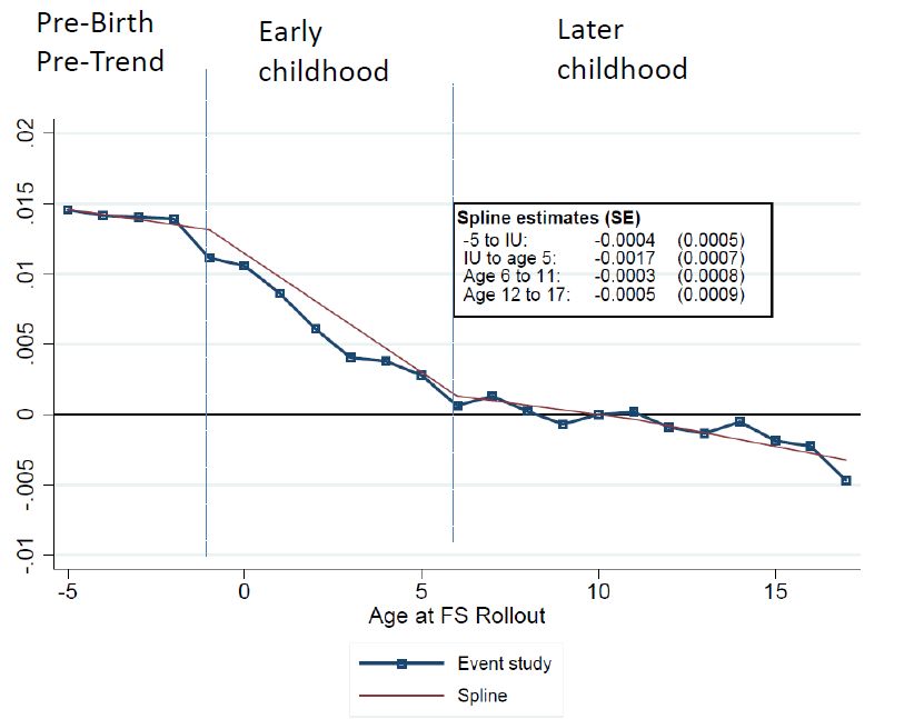

Long run impacts of early life shocks or interventions?
Why do we need movement in the data frontier?

    • How long do the impacts of these interventions last?
    • requires interventions that are “old enough” so we can follow
      treated cohorts over time
    • many large US education and welfare experiments happened in
      the 1970s and 1980s
    • those treated then are now around age 30-40, so impacts on
      completed education, earnings and other adult outcomes can be
      analysed → this has led to a surge in studies examining
      longer-run impacts of such policies
    • prior work used small survey data (PSID), often with a limited set
      of available outcomes

c Royal Holloway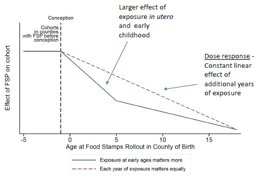

Long run health impacts of early life interventions?

    • health and mortality impacts tend to manifest later
    • severe health shocks tend to be more prevalent from about age 50
    • need about 6-7 decades of data and large samples for adequate
      statistical power

             Figure: Mortality rates by age, UK, cohorts born 1944 to 1955

c Royal Holloway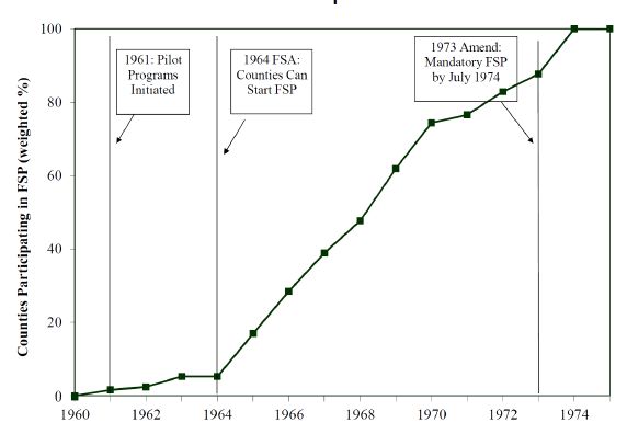

A seminal model of health capital - Grossman (1972)

    Components:
    • it’s an old seminal paper, but...
    • it is a useful conceptual framework for studying
            •   ...   most aspects of the demand for health
            •   ...   understanding sources of health inequalities
            •   ...   income and price impacts on the demand for health
            •   ...   the design of public health programmes, interventions

c Royal Holloway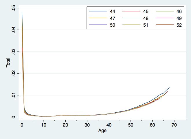

The Grossman model

    Components:
    • human capital model of the demand for health
    • health is
           1. a stock
           2. a choice (enters the utility function)
           3. produced by the individual

    Intuition:
    • health is a durable capital stock that yields healthy time as
      service flow
    • stock depreciates with age and increases with investment
    • health investments crowd out time for other activities, i.e. market
      work and leisure, and other consumption

c Royal Holloway

The Grossman model - utility

    Two goods: healthy time ht , other consumption Zt

    Intertemporal utility function

                                U = U(ht , Zt )

    where

    ht = φt Ht is consumption of health services (or healthy time) Ht :
    stock of health at t
    φt : service flow per per unit of health stock health at t

c Royal Holloway

The Grossman model - investment

    Net investment in health in t is

                           Ht+1 − Ht = It − δt Ht

    Assumption: δt is exogenous but increasing in age

c Royal Holloway

The Grossman model - production

    Individuals use time (and input goods) to produce health and other
    consumables according to the following production functions:

                            It = It (Mt , THt ; E )

                            Zt = Zt (Xt , Tt ; E )

    M,X: endogenous goods inputs
    TH,T: endogenous time inputs
    E:    consumer’s exogenous stock of knowledge (education)

    Note: there is no joint production using the same inputs here
    (e.g. vegetables may be M or X, and both affect I and Z)

c Royal Holloway

The Grossman model - constraints

       n                 n
       X pt Mt + qt Xt   X ωt TWt
                    t
                       =             + A0             Budget constraint (1)
            (1 + r )       (1 + r )t
        t=0                     t=0

                   p,q:   prices
                   TW:     hrs of work
                   ω:      wage
                   A0 :   initial assets
                   r:     interest rate

               TWt + THt + Tt + TLt = Ω               Time constraint   (2)
                   TL:    time lost through illness
                   Ω:       total time
c Royal Holloway

The Grossman model

    Substituting into BC:

      n                                       n
      X pt Mt + qt Xt + ωt (THt + Tt + TLt ) X ωt Ω
                                            =             + A0 (3)
                       (1 + r )t                (1 + r )t
       t=0                                   t=0

    Assumptions:

                              ∂TLt

The Grossman model - equilibrium conditions

                                ωt Gt        (1−δt )ωt+1 Gt+1             (1−δt )...(1−δn−1 )ωn Gn
                               (1+r )t   +      (1+r )t+1
                                                                + ... +            (1+r )n
              πt−1
                       =                                                                       (6)
           (1 + r )t−1
                                  + Uh                                     Uhn
           | {z }
                                     λ Gt + ... + (1 − δt ) ... (1 − δn−1 ) λ Gn
                                       t
           PDV of MHC
                           |                           {z                                            }
                                                         PDV of MHB

c Royal Holloway

PDV of MC of gross investment:

    depends on ...
    • the interest rate r
    • MC of gross investment, πt−1 , which is a function
                                       pt−1            ωt−1
                          πt−1 =                =                                  (7)
                                   ∂It−1 /∂Mt−1   ∂It−1 /∂THt−1

        of

             •   the price p of health inputs M
             •   the MP of input in the production of health, or, alternatively,
             •   the price of the time input TH, ω
             •   and the MP of TH into production of H

c Royal Holloway

PDV of marginal health benefit

    The marginal benefit of gross health investment in t:
                                    
                   ωt         +
                                 Uht 
                                               ·        Gt                       (8)
                    (1 + r )t     λ                    |{z}
                    |       {z      }            MP of health capital
                   discounted marginal value of of health capital

    which depends on
    • λ: MU of wealth
    • discounted wage rate (value of a unit increase in market time)
                                ∂U
    • Uht : MU of healthy time ∂h
                                                 t
                                                                    ∂ht
    • Gt : MP of health stock in healthy time production            ∂Ht   = − ∂TL
                                                                              ∂Ht
                                                                                  t

c Royal Holloway

Interpretation

    • Equation 6 determines optimal gross investment in t-1
    • Equation 7: cost is minimised when the relative price of both
      inputs (time, goods) equals the ratio of marginal productivities

    Note: AC of gross investment is constant and equal to MC due to
    • homogeneous production functions
    • prices that do not depend on the stock (or on age)

c Royal Holloway

Optimal health stock in t

    Optimal investment (not discounted)
                                    
                       Uht         t
              Gt ωt +      (1 + r ) = πt−1 (r − πg
                                                 t−1 + δt )         (9)
                         λ

    must equal rental (or user) cost of health capital,
    which depends on
    • interest rate
    • depreciation rate
    • percentage rate of change in marginal cost between period t - 1
      and period t ≈ 0

c Royal Holloway

Model predictions

    Reduction in price of medical care p

    • substitute medical care for other health inputs (here: time; in an
      extended model may also be self-care or own private medical
      expenses) due to change in relative prices (SE)
    • hold more health capital (IE)

    Increase in wages (incomes) ω
    • increases opportunity cost of time, induces lower time investment
      in health stock (SE)
    • hold more health capital (IE)
    • raises return on a healthy day → increases health capital

c Royal Holloway

Model predictions

    Increase in age (here equal to t)

    • if depreciation rate is (constant) increases in age, then rental
      price of health goes up (is constant), so health investment
      decreases (remains unchanged)
    • yet, health stock depreciates quicker, hence while health stock
      goes down, health investments may not
      (in fact, empirically, health expenditure increases in age)

c Royal Holloway

Model predictions

    Increase in educational attainment Under the assumption that more

    educated people are better at producing of health capital (higher
    productivity), i.e.
    • they are better able to determine high-yield health investments
      (prevention, timing of doctor visits, types of treatments)
    • they have a larger health stock
    • but not clear whether they invest more
    • (education also affects wages)

c Royal Holloway

Possible extensions: see here for details

   1. Uncertainty: health insurance to smooth unexpected shocks
      → shocks could be introduced via stochastic depreciation rate or
      stochastic future earnings

   2. Individual heterogeneity:
            •   depreciation rates
            •   initial health stocks
            •   productivity in producing health
            •   preference

   3. Differential mortality: role of genetics, early (in utero) health
      environments,...

c Royal Holloway

Possible extensions

   4. Health production function:
            • Multiple inputs: private vs. public health care, out-of pocket
              expenditure, health lifestyle...
            • Joint production: there may be joint production of healthy time
              and consumption (e.g. vegetable cons., sports,...)
            • constant returns to scale in health production: some lack of health
              investment may be irreversible, marginal productivity of health
              investment may be decreasing in age...

c Royal Holloway

Possible extensions

   5. Perfect foresight:
      → Over (under-) investment into health due to different
      information set about health risks, and benefits of health
      investments
      → diagnosis process or doctor visits may be informative about
      health stock and the health production function → learning about
      returns to health investments

   6. Rationality: no role for bounded rationality
      → people may be perfectly informed but find it hard to adjust
      their behaviour
      → time inconsistency: hyperbolic discounting where future
      benefits are weighted down in the short-run (present bias)
      → rational addiction models: Adda and Cornaglia (2010)
      → rational inattention, other behaviouristic biases?
c Royal Holloway

Implications for research and policy?

    • Private health investment will depend on the price of medical care
      or other health-relevant expenses (cigarettes and unhealthy foods,
      medical care and health-enhancing consumer goods, disease
      prevention,...)
    • income growth is likely going to lead to better health Figure
    • if individuals do not have perfect information, then there may be
      scope for:
            • information interventions (5 a day campaign, vaccination
              information,...)
            • some routine interventions like free prevention, health check offers
            • behavioural interventions (habit formation, ...)

    • Timing may matter in health investments: role for childhood
      interventions

c Royal Holloway

The Grossman model and early life health interventions
or: How may early childhood health environments shape adult health?

    Early, more severe decumulation of health stock (than at older ages)
    or lack of reaching potential health stock
    • Infancy is a key development period → differential return to health
      investments (loss of stock due to shocks) in different periods?

    Depreciation rate
    • Early life illness may inhibit neurological development in infancy,
      accelerating aging process (Bhalotra and Venkataramani, 2013)
      → increase in depreciation rate throughout the life cycle

    • Biological embedding (Shonkoff et al., 2009)
      Immature “organism” adapts to key environmental characteristics,
      and retains initial programming, even when environment changes
      → irreversible change in health stock?
c Royal Holloway

Important historic early life interventions

      Program                              Start year   Impacts
      Education interventions
      Perry preschool                      1970         Website
      Head Start                           1965         Garces, Thomas, Currie (2002)

      Nutrition & health interventions
      Food Stamps (SNAP)                   1962-75      Hoynes, Schanzenbach, Almond (
      Medicaid intro                       1970         Goodman-Bacon (2018, 2017)
                expansions                 80s, 90s     Brown et al. (2015)
                                                        Wherry and Meyer (2016)
                                                        Currie and Gruber (1996)
                                                        Currie et al. (2008)
      NHS intro                            1948         Luhrmann and Wilson (2020)
      Scandinavian Well-Child Programmes   1930s        Bhalotra, Karlsson, Nilsson (2017
                                                        Bütikofer, Løken, Salvanes (2018
                                                        Hjort, Sølvsten, Wüst (2017), Wu

    European health systems and welfare programmes tend to be older
    than those in the US...
c Royal Holloway

Typical identification strategies used in these studies

    • difference-in-difference model or regression discontinuity design
    • exploiting cohort-specific exposure to welfare programme or
      health intervention, combined with geographic variation from
      staggered rollout (in US states)
    • Example: long run impact of SNAP - a large US welfare
      programme - Hoynes et al (2016)
      difference-in-difference approach

c Royal Holloway

SNAP, formerly food stamps programme

    • 40.3 million recipients in 20 million households (2018)
    • average monthly benefit of USD 252 per household
    • delivered in vouchers that can be used in grocery stores
    • means testing: requires gross monthly income below 130% of
      poverty line
    • third largest US welfare programme in terms of expenditure (after
      Medicaid and EITC)

c Royal Holloway

What is the link between SNAP and health?

    • SNAP is a conditional cash transfer programme
    • it conditions on the transfer being spent on food
    • healthy nutrition is emerging as a key factor in early life
      interventions
    • cash and conditional cash transfer programmes have been
      extensively used to buffer individual shocks during the COVID-19
      pandemic
            • e.g. SNAP
            • voucher system to compensate for (unavailable) free school meals
              in the UK (affects 1.3 million children)
            • direct payout of missed school meals in the US: about 120 USD
              per month and child (affects 30 million students who receive free
              or reduced price school meals)

c Royal Holloway

Challenges to identification in SNAP

    • universal programme
    • federally administered (little variation in generosity across states)
    • few reforms
    • negative selection: typically receive SNAP when adverse shock
      hits

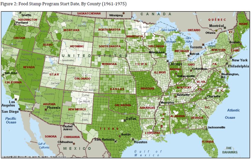
c Royal Holloway

Hoynes et al. (2016): staggered rollout of FSP

    Also used in Bailey et al. (2020)
c Royal Holloway

Hoynes et al. (2016): Staggered rollout of FSP

c Royal Holloway

Hoynes et al. (2016): difference-in-difference approach

    Compare adult outcomes for those with early childhood exposure to
    FSP in their county of birth to those born earlier (and therefore
    without childhood FSP exposure)

      yibc = α + δTc,b + Xibc β + ηc + λb + γt + θs · b + ρZc60 · b + ibc (10)

    where
    T : childhood FSP exposure (share of months FS available between
    conception and age 5 in birth county)
    b: cohort
    c: geography (here:county)
    s: state

c Royal Holloway

Hoynes et al. (2016): identifying assumptions

    • exogeneous introduction of FSP across counties
      → empirically: control for trends in the observable determinants
      of FSP adoption by including interactions between characteristics
      of the county of birth and linear trends in year of birth CB60g · c

    • common trend assumption: no competing welfare programs rolled
      out with similar staggering
      → control for county of birth characteristics (community health
      centers, hospitals and hospital beds per capita, and non-FSP
      government transfers per capita), measured as averages over the
      first five years of life.

c Royal Holloway

Hoynes et al (2009): impact of childhood safety net on
adult outcomes
    • examine change in economic resources available in utero and
      during childhood (up to age 5)
    • Food Stamp Program, rolled out across counties in the U.S.
      between 1961 and 1975.
    • Data: PSID (incl. county of birth information)
    •      3000 nationally representative hhs + 1900 low income and
      minority hhs
    •      combine with USDA annual reports on county FSP caseloads
      per county and year to construct childhood FSP exposure (share
      of time between conception and age 5 that FSP is available in
      birth county)
    •      oldest individuals can be followed up to age 53
    •      control for county characteristics
    •      good earnings, income and education information and some
      health information (summarised in metabolic health index)
c Royal Holloway

FSP exposure - timing effects?

    • Does the timing matter? Are returns of SNAP different
      depending on when benefits were received between age 0 and 5?

c Royal Holloway

Hoynes et al (2009): findings

    • childhood outcomes (Hoynes and Schanzenbach, 2009)
            • introduction of FSP increased householdsspending on food
            • increase in economic resources rather than nutrition programme
            • pregnancies exposed to FSP three months prior to birth yielded
              deliveries with increased birth weight
            • largest gains at the lowest birth weights; larger impacts for African
              American mothers
    • adult outcomes
            • food stamp program has effects decades after initial exposure
            • greater exposure to FSP before age 4-5 significantly reduces the
              incidence of adult metabolic syndrome (obesity, high blood
              pressure, and diabetes)
            • for women, an increase in economic self-sufficiency

c Royal Holloway

Followup paper: Bailey et al. (2020)

    • move to large linked dataset of survey-administrative data (> 17
      million households)
    • Social security data linked with census records
    • examine a comprehensive set of outcomes such as human capital,
      disability, mortality, incarceration
    • aggregate to birth county x birth year x survey year cells (partially
      also by race and sex)
    • but: loose information on socio-economic status (education,
      poverty) and shorter time horizon (up to age 33)
    • take into account impact of complementary welfare programs
      (EITC, Community Health Centers, WIC)

c Royal Holloway

Bailey et al. (2020) - econometric specification

                                               a=17
                                               X
    ycbt = ηc +δs(c)b +γt +Xcbt β+Zc60 bρ+                πa ·1[b−FSc = a]+cbt
                                            a=−5[a6=10]
                                                                       (11)
    where
    ηc : birthcounty FE
    δs(c)b : birth state x year FE
    Xcbt : cohort-county-year FE (all at birth)
    Zc60 b: 1960 county characteristics x linear birth cohort
    FSc : year FSP was first available in county c
    a: age when FSP was first introduced
    πa : event time coefficients, ranging from 5 years before birth to age
    17 (age 10 omitted category)

c Royal Holloway

Bailey et al. (2020) - hypotheses
    • If no pre-trends: pi should not be statistically significant for
      a < −1 (conception)
    • If earlier investment have larger returns, then π̂a should be largest
      in utero and early childhood (a=-1 to 5)
    • Estimate spline function:
                   ycbt =ηc + δs(c)b + γt + Xcbt β + Zc60 bρ
                         + ω1 1[b − FSc < −1] · (b − FSc )
                           |             {z             }
                               FS pre-conception (pre-trends)

                         + ω2 1[−1 ≤ b − FSc < 6] · (b − FSc )
                           |              {z                }
                                  FS in utero & early childhood       (12)
                         + ω3 1[7 ≤ b − FSc < 11] · (b − FSc )
                           |               {z               }
                                          FS age 6-11

                         + ω4 1[12 < b − FSc ] · (b − FSc ) +cbt
                           |             {z              }
                                       FS age 12-17
c Royal Holloway

Robustness checks

    • test for pre-trends (see above)
    • county adoption timing voluntary =? endogenous?
            • balancing test
            • birth county-corth year controls (population, mortality rates,
              complementary welfare programme rollout)
            • flexible Xcbt terms (birth cohort-county-year FE (all at birth)
            • pre-trends

c Royal Holloway

Bailey et al. (2020) - does the timing of FSP receipt
matter?

c Royal Holloway

Bailey et al. (2020) - magnitude of results

    Implies: 5yr + IU exposure → 0.009 SD increase in composite index
    similar results in spine model: 5.75 years x 0.0017=0.0098

c Royal Holloway

Bailey et al. (2020) - a few additional results

    • 7% TOT impact on earnings
    • 0.06 SD in human capital index
    • 11% reduction in mortality
    • Largest impacts on human capital, esp. years of schooling and
      attending college
    • ...concentrate among whites, particularly males
    • survival gains concentrated among non-whites
    • reductions in incarceration among non-whites (only)

c Royal Holloway

Bütikofer et al. (2019): long-run impact of infant health
care centers

    • treatment: well-child visits include physical examination and
      information on adequate nutrition (breastfeeding)
    • DiD; similar in method to Hoynes et al.
    • use the variation in exposure to infant health care services driven
      by mother and child health care center openings, and the scope of
      the services provided
    • exploit the rollout of newly established mother and child health
      care centers across municipalities over time.

c Royal Holloway

Bütikofer et al. (2019): difference-in-difference approach

    • DiD; similar in method to Hoynes et al.
    • use the variation in exposure to infant health care services driven
      by mother and child health care center openings, and the scope of
      the services provided
    • exploit the rollout of newly established mother and child health
      care centers across municipalities over time.
    • data: Norwegian registry data, combined with historic data on
      center rollout
    • health data: Cohort of Norway (CONOR) data and the National
      Health Screening Service’s Age 40 Program data

c Royal Holloway

Bütikofer et al. (2019): robustness

    • similar identifying assumptions
    • test whether municipality characteristics predict center opening
    • use sibling fixed effects to show that results are not driven by
      selective migration into municipalities with early centers

c Royal Holloway

Bütikofer et al. (2019): findings

    • access to mother and child health care centers in the first year of
      life increased
            • completed years of schooling by 0.15 years
            • earnings by two percent.
            • effects were stronger for children from a low socioeconomic
              background
            • 10 percent reduction in the persistence of educational attainment
              across generations.
            • positive effects on adult height and fewer health risks at age 40

    • immediate effect: access to well-child visits decreased infant
      mortality from diarrhea whereas infant mortality from pneumonia,
      tuberculosis, or congenital malformations are not affected
    • mechanism: better nutrition

c Royal Holloway

Long-run Health and Mortality Eects of Exposure to
             Universal Health Care in Infancy
         Melanie Lührmann (Royal Holloway and IFS) and Tanya Wilson
                             (University of Glasgow)

        Acknowledgement: British Academy/Leverhulme SG162230 & BA MF170399

1 /36

Disclaimer

     The permission of the Oce for National Statistics to use the
     Longitudinal Study is gratefully acknowledged, as is the help provided by
     sta of the Centre for Longitudinal Study Information & User Support
     (CeLSIUS). CeLSIUS is supported by the ESRC Census of Population
     Programme (Award Ref: ES/K000365/1). The authors alone are
     responsible for the interpretation of the data.

     This work contains statistical data from ONS which is Crown Copyright.
     The use of the ONS statistical data in this work does not imply the
     endorsement of the ONS in relation to the interpretation or analysis of
     the statistical data. This work uses research datasets which may not
     exactly reproduce National Statistics aggregates.

 2 /36

Motivation

    Impact of infancy exposure to universal healthcare on mortality and
    health around ages 50-60

        •   Intervention:

            NHS introduction in 1948

        •   We digitised historical data sources to investigate the
            immediate impact of the NHS on infant survival

        •   For longer-term outcomes we use a RD design enriched with
            geographical variation in medical services provision for
            identication.

        •   impacts are estimated using large administrative datasets
            recording death and hospitalisation

3 /36

Related evidence: Medicaid introduction (1960s) and
expansions (1980s-90s)
         •   Short run: reductions of

               • perinatal (before birth and death < 7 days) and
               • neonatal (death < 28 days) mortality
                 Goodman-Bacon (2018), Currie and Gruber (1996a,b)

         •   Medium run: improvements in
               • childhood and adolescent health
               • educational attainment
               • better early labour market outcomes, higher tax receipts, lower
                 welfare dependency
                 Currie et al. (2008), Brown et al. (2015), Wherry and Meyer
                 (2016)

         •   Vietnam UHC led to signicant increase in utilization of public
             health services among eligible children (Vu 2019; Nguyen and
             Wang, 2012)
 4 /36

Institutional Setting: Pre-NHS

         •   Mainly private provision

         •   National Insurance Act (1911)

               • rudimentary medical care provided to employed persons aged
                   16-70 with annual earnings below a threshold
               •   Coverage did not extend to dependents

         •   Limited access to free healthcare by LAs and vol. hospitals
             (under severe nancing problems by 1940s)

 5 /36

Institutional setting: NHS

         •   1942: Beveridge report highlights social and health disparities
             in the UK

         •   July 1948: introduction of universal healthcare via the
             National Health Service

         •   Aims of the NHS:

               • equalisation of access to medical services
               • free at the point of use
               • access is based on clinical need, not ability to pay

 6 /36

Institutional setting: NHS
     After fraught negotiations, family doctors (GPs) agreed to
     participate on 28th May 1948.

     Large-scale information campaign began June 1948

 7 /36

Institutional setting: NHS

     Within 5 months 96% of population had signed up to the NHS:

         •   6th July: 35,757,997 people registered (84%)

         •   31st July: 38,669,195 (91%)

         •   30th Oct: 40,706,290 (95%)

         •   31st Dec: 41,466,755 (96%)

     By Sept, 18,165 out of 21,000 GPs had signed up (87%)

 8 /36

Institutional setting: NHS

     Initially not accompanied by a large investment programme to
     boost resources (no new hospitals, no discontinuous expansion in
     doctors or nurses)

         •   hospitals were centralised

         •   doctors became independent contractors

         •   local authorities continued to administer family health services

 9 /36

Institutional setting: Distributional changes in services
utilisation
     There can be little doubt that before the start of the new National
     Health Service many women [...] were deterred from seeking
     medical advice by economic reasons. Now that the nancial barrier
     has been removed, women [...] are able to consult their doctor
     more often than they did before. (Logan, 1950, Lancet)

10 /36                     Source: Survey of Sickness, The Wellcome Library.

Immediate eects: Infant mortality data

     We use data digitised from Registrar General's Statistical Review of
     England and Wales, and from Ministry of Health Annual Reports.
     Detailed population data on mortality in infancy by:

         •   period 1943 to 1953

         •   county

         •   subperiods of death
             (pre-, neo- and postneonatal death rates up to 1 year)

         •   cause of death

         •   marriage status of the mother (legitimacy)

11 /36

Immediate eects
Pre-natal mortality and mortality at birth

     No evidence of a discontinuity in

         •   maternal mortality

         •   stillbirths

         •   mortality around delivery (rst 30 minutes, rst day)

     →   results not suggestive of improvements in ante-natal services
     →   no NHS impact at delivery

12 /36

Immediate eects: Infant mortality data
     Reduction in infant mortality (17%) is predominantly driven by
     large declines in the neo-natal period...

                   Source: Registrar General's Annual report 1940-1955, The Wellcome Library.   by week

13 /36

Immediate eects: Infant mortality data
     .. due to prevention of deaths from acute conditions (pneumonia
     and diarrhea)...
     .. with lasting eects on human capital accumulation, employment
     and earnings (Bhalotra and Venkataramani, 2013, 2015)

                 (a) Diarrhea                                               (b) Pneumonia
                        Source: Ministry of Health Annual Reports, The Wellcome Library.

14 /36

Immediate eects: Infant mortality data
     .. and concentrated among individuals of lower socio-economic
     status who prior to the NHS had low or no access to healthcare

                    Source: Registrar General's Annual report 1940-1955, The Wellcome Library.

15 /36

Robustness of infant mortality results
     That the fall in infant mortality is associated with increased access
     to medical services via the NHS is consistent with Dykes (1950)

         •   Case study of a large town in 1946 - nds strong SES gradient
             in infant mortality
         •   Higher mortality related to delay in accessing medical care

     Examination of other factors inuencing infant mortality revealed
     no sharp discontinuity in:

         •   breastfeeding practices
         •   availability of vaccinations/food (rationing)

     Also investigated other potential drivers:

         •   changes in birth trends/composition of births (by age/parity)
         •   weather (`hard' winters)
         •   Infant mortality trends in other countries

16 /36

Adult mortality data

     ONS Longitudinal Study

         •   administrative data from ve successive linked censuses
             (1971-2011)

         •   census panel is linked to death records up to 2015
             with information on time and cause of death

         •   approximate 1% sample of the population of England and
             Wales

         •   data contains rich set of socio-economic characteristics

         •   ...and location at birth

     combined with GBHD data on social class composition          SES

17 /36

Identication strategy I

            method fuzzy RD design

           threshold birth in 1948 (UK Biobank: month and year of birth)

            window cohorts born between 1945 and 1951

               fuzzy probability of an increase in pre- or postnatal care is a
                     function of socio-economic status

     birth county FE capturing local economic conditions & healthcare
                     infrastructure

         yicg = α + βCc + γ1 Tc + γ2 Tc LCic + δLCic + Xic0 η + µg + ic   (1)

18 /36

Estimates of mortality rate, I

                     Table: Estimates of mortality rates by ages 52 to 64
                                                                Mortality rate by age ...

                             52             54               56           58          60          62          64

         Tc ∗ LCic       -0.0173**    -0.0223**        -0.0187**      -0.0249**   -0.0279***   -0.0272**   -0.0313***
                         (0.00763)    (0.00874)        (0.00875)      (0.00998)    (0.0100)    (0.0104)     (0.0112)

         Tc              0.00678*     0.00897**            0.00560     0.00697      0.0102*    0.00935*     0.00816
                         (0.00392)    (0.00426)        (0.00482)      (0.00512)    (0.00536)   (0.00530)   (0.00617)

         Observations     44,121           44,121          44,121       44,121      44,121      44,121      44,121
         F-test for joint signicance of   Tc LCic   and   Tc   coecients
         p-value          0.0790*      0.0391**            0.1057      0.0509*     0.0244**    0.0347**    0.0262**
         Mean mortality rate prior to NHS inception, by social class
         LC               0.0488           0.0606          0.0730       0.0884      0.1029      0.1209      0.1421
         HC               0.0306           0.0367          0.0462       0.0558      0.0657      0.0783      0.0899
         Mortality reduction in percent (relative to mean), by social class
         LC                -21.56          -22.00      (-17.95)         -20.28      -17.20      -14.76       -16.28
         HC                22.16           24.44           (12.12)      (12.49)      15.53       11.94       (9.08)

19 /36

Geographical variation in medical services
Identication strategy II

         •   NHS: free healthcare in a rationed needs-based system     →
             increased patient competition for healthcare

         •   Recall: no supply change at NHS introduction, i.e. short-run
             xed resource

         •   County-level per capita medical services   mi   determined by the
             fraction of population who could aord access pre-NHS

         •   Higher county proportion of insured individuals (pre-NHS)

                 → county medical services per capita in 1948 ↑
                 → proportion of new patients demanding healthcare ↓

         •   proxy proportion of insured through county-level social class
             composition

20 /36

Geographical variation in medical services
Evidence

                    Source: The Hospital Surveys, HMSO; GBHD database.

21 /36

Geographical variation in medical services
Evidence

                     Source: First General Practice Committee Report.

22 /36

Identication strategy II

     We proxy inow of new patients through county-level social class
     composition (proportion of insured):

                         yicg = α + βCc + γ1 Tc + γ2 Tc LCic
                   +γ3 Tc HIGHareag + γ4 Tc LCic HIGHareag
                                                                        (2)
                 +γ5 LCic HIGHareag + δLCic + ζHIGHareag
                                                 +Xic0 η + ic

         HIGHareag :   area with a high (upper tertile) proportion of
         previously insured (→ low inow of new patients)

23 /36

Estimates of mortality rate, II
                                                          Mortality rate by age ...

                                 52           54          56           58           60             62       64

         Tc ∗ LCic            -0.0119       -0.0110     -0.0128     -0.0227*     -0.0224     -0.0303**    -0.0271
         ∗ HIGHarea           (0.0124)     (0.0118)    (0.0125)     (0.0118)     (0.0140)    (0.0150)    (0.0196)

         Tc ∗ LCic           -0.0158**     -0.0211**   -0.0172*    -0.0217**    -0.0243**    -0.0225**   -0.0272**
                             (0.00751)     (0.00854)   (0.00861)    (0.0102)     (0.0101)    (0.0106)    (0.0111)

         Tc ∗   HIGHarea    -0.00825**     -0.00598    -0.0108**   -0.00763*     -0.00453    -0.00344    -0.00254
                             (0.00318)     (0.00361)   (0.00520)   (0.00441)    (0.00428)    (0.00473)   (0.00529)

         Tc                  0.00845**     0.0102**     0.00770     0.00852      0.0110**     0.0101*    0.00873
                             (0.00412)     (0.00433)   (0.00480)   (0.00521)    (0.00532)    (0.00526)   (0.00619)

         Observations          44,121       44,121      44,121       44,121       44,121      44,121      44,121
         F-tests of joint signicance (p-values)
         LC in HIGHarea       0.0519*       0.0838*    0.0208**     0.0169**     0.0532*     0.0429**    0.0808*
         LC in LOWarea        0.0751*      0.0338**     0.1275      0.0988*      0.0397**     0.0700*    0.0534*
         HC in HIGHarea       0.0280**     0.0493**     0.0628*      0.1200      0.0943*      0.1488      0.3607

         Mortality change in percent (relative to mean mortality rate), by area and social class
         LC in HIGHarea        -44.07        -39.83      -38.13      -42.04       -33.89       -32.96     -29.83
         LC in LOWarea         -17.13        -19.60      -14.42      -16.19       -13.93       -11.01     -13.32
         HC in HIGHarea         0.61         11.92       -6.71       (1.61)       10.13        (9.00)      7.21
         HC in LOWarea         29.86         32.69      (18.08)      (16.17)      17.43        13.43       9.60

24 /36

Estimates of mortality rate, II

     Higher mortality reductions

         •   for low SES born in High SES areas

         •   in High SES areas

         •   amongst low SES

     ... but crowding out eects of patient inow on those with previous
     access to healthcare

         •   that rise in the scarcity of available medical services

25 /36

Conclusion

         1. Infancy access to UHC strongly reduces infant mortality
             (-17%)

         2. Does it have a long-run impact on health and mortality 50-60
             years after exposure?
         3. Yes, evidence of mortality reduction (and, using Biobank data,
             reduction in the onset of cardiovascular disease)

               • ...among individuals with low or no access to medical services
                  prior to the NHS.
               • ...and larger reductions among lower SES individuals in areas
                  with more medical services per person.

     However, evidence of adverse eect for those who would have had
     access to healthcare without the NHS

         •   Survival gains for former group larger than mortality increases
             of latter

26 /36

Implications for public policy

         •   Access to universal healthcare in infancy yields benets across
             almost the entire lifetime into older ages

               • benets of early childhood interventions can be underestimated
               • informative for recent universal healthcare programmes (UN)

         •   But....

               • introducing a UHC system without accompanying investments
                  in healthcare infrastructure increases competition among
                  patients
               • This can lead to adverse eects (through access to fewer
                  medical services in infancy) for those who had access under the
                  previous system.

27 /36

Conclusions

    • childhood environments matter...
    • ...and their long-run effects are a productive field of research:
           1. ample evidence that timing of redistributive interventions matters
           2. health research benefits in particular from increasingly available
              administrative data
           3. Europe’s welfare systems developed early
           4. open questions around health capital accumulation (and its
              interaction with other forms of human capital)
           5. emerging knowledge into long term effects
              ...and wether they can be predicted using indicators in early and
              middle childhood
           6. mechanisms and life cycle pathway of impacts: what happens in
              the “missing middle” years?
           7. literature has mostly focused on shocks - shift towards public
              policies (positive environment changes) that may help reduce early
              life inequalities

c Royal Holloway

Mortality and income   back

c Royal Holloway