Cooperative Manipulation and Transportation with Aerial Robots

Page created by Jorge Sims
 
CONTINUE READING
Cooperative Manipulation and Transportation with Aerial Robots
Cooperative Manipulation and Transportation
                     with Aerial Robots
                                     Nathan Michael, Jonathan Fink, and Vijay Kumar
                                                University of Pennsylvania
                                                Philadelphia, Pennsylvania
                                    Email: {nmichael, jonfink, kumar}@grasp.upenn.edu

   Abstract—In this paper we consider the problem of controlling
multiple robots manipulating and transporting a payload in                            q1                    qi
three dimensions via cables. We develop robot configurations
that ensure static equilibrium of the payload at a desired pose                                                  li
                                                                                            l1
while respecting constraints on the tension and provide analysis                       g
of payload stability for these configurations. We demonstrate                                          pi
our methods on a team of aerial robots via simulation and                                                    C
                                                                                                                                qn
experimentation.                                                                                       r                ln
                                                                                      W
                      I. I NTRODUCTION
   Aerial transport of payloads by towed cables is common in
emergency response, industrial, and military applications for
object transport to environments inaccessible by other means.
                                                                     Fig. 1. A rigid body suspended by n cables with world-frame pivot points qi .
Examples of aerial towing range from emergency rescue                Analysis techniques for cable-actuated parallel manipulators assume that qi is
missions where individuals are lifted from dangerous situations      fixed while li varies in magnitude, while for cooperative aerial manipulation
to the delivery of heavy equipment to the top of a tall building.    we fix li and vary qi by changing the positions of the aerial robots.
Typically, aerial towing is accomplished via a single cable
attached to a payload. However, only limited controllability         is affected by robot positions and in the latter pose control
of the payload is achievable with a single attachment point          is accomplished by varying the lengths of multiple cable
[1].                                                                 attachments (see Fig. 1). Thus the work on workspace analysis
   In this work we address the limitations of aerial towing by       [3, 4], control [5], and static analysis [6] of such parallel
designing cooperative control laws for multiple aerial robots        manipulators is directly relevant to this paper.
that enable manipulation of a payload in three dimensions.              More generally, we are interested in the mechanics of pay-
While we formulate the general conditions for system equi-           loads suspended by n cables in three dimensions. The n = 6
librium at the desired pose for an arbitrary number of robots,       case is addressed in the literature on cable-actuated platforms.
we focus on a system of three aerial robots for discussions of       When n = 5, if the line vectors are linearly independent and
workspace and payload stability. We show that despite the fact       the cables are taut, the line vectors and the gravity wrench
that such a system is underactuated and limited by unilateral        axis must belong to the same linear complex [7]. The payload
tension constraints, we are able to manipulate a payload to          is free to instantaneously twist about the reciprocal screw
a desired pose (position and orientation) in simulation and          axis. When n = 4, under similar assumptions on linear
experimentation. We extend the analysis to motion planning           independence and positive tension, the line vectors and the
by exploring the set of possible robot configurations for a given    gravity wrench must belong to the same linear congruence.
payload pose.                                                        The unconstrained freedoms correspond (instantaneously) to
   While examples of cooperative multi-robot planar towing           a set of twists whose axes lie on a cylindroid. In the n = 3
exist in the literature, there are significant differences between   case, all three cables and the gravity wrench axis must lie
interacting with an object on the ground and in the air. In [2],     on the same regulus - the generators of a hyperboloid which
the authors consider the problem of cooperative towing with a        is a ruled surface [8]. Of course, in all of these cases there
team of ground robots, where under quasi-static assumptions          are special configurations in which the screw systems assume
there is a unique solution to the motion of the object given         special forms [7] which are not discussed in this paper. The
the robot motions. This approach is not directly extensible to       arguments for the n = 1 and the n = 2 cases are similar, but
three-dimensional manipulation where frictional ground forces        in these cases, the cables and the center of mass must lie on
are absent and gravity introduces dynamics into the problem.         the same vertical plane for equilibrium.
   The cooperative aerial towing problem is similar to the              We approach the development of controllers for cooperative
problem of controlling cable-actuated parallel manipulators          aerial manipulation and transportation as follows: in Sect. II
in three dimensions, where in the former the payload pose            we formulate conditions for general static equilibrium of an
Cooperative Manipulation and Transportation with Aerial Robots
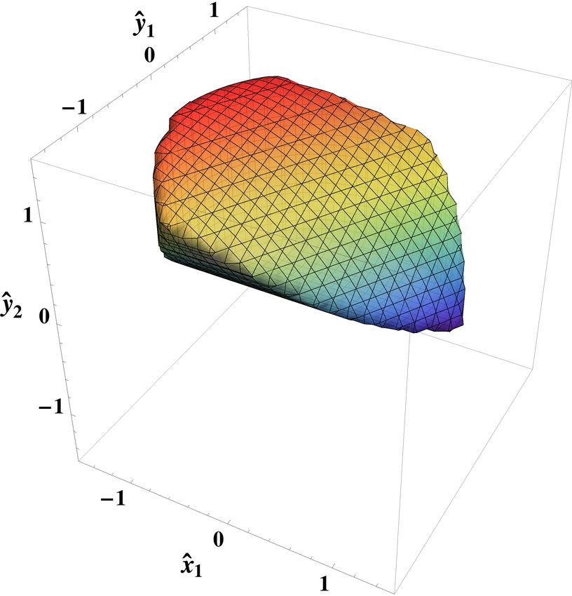
object in three dimensions, after which we focus our discus-                               z̃ = 1
                                                                                                                     q̂3
sion on systems with three robots. By deriving conditions
                                                                                              q̂1                          q3
of static equilibrium and analyzing these conditions based                                                                      q̂2
                                                                                                           ŷ
on bounded tension models and stability, in Sect. III we                                            q1          x̂
are able to identify valid system configurations for aerial                                                                       q2
manipulation that ensure that the payload achieves a desired
                                                                                                          B P3
pose. Through simplifying assumptions guided by our robot                                                   ỹ
                                                                                                         P1       P2
model, we are able to arrive at closed-form analytic solutions                            W                    x̃
for the tensions in the cables and payload stability for a given
                                                                                                         A
system configuration. For the derivation of valid configurations
we assume point-model robots. In Sect. IV, we develop and
experimentally validate controllers for dynamic robots that
respect this point-model and enable application of our methods          Fig. 2. A team of three point-model robots manipulate a payload in three
to a team of quadrotors. We review and analyze simulation               dimensions. The coordinates of the robots in the inertial frame W are qi =
                                                                        [xi , yi , zi ] and in the body-fixed frame (attached to the payload) B are q̃i =
and experimental results in Sects. V and VI and conclude in             [x̃i , ỹi , z̃i ]. The rigid body transformation from B to W is A ∈ SE(3).
Sect. VII.                                                              Additionally, we denote the projection of the robot position q̃i along qi − pi
                                                                        to the plane z̃ = 1 as q̂i = [x̂i , ŷi , 1].
                II. P ROBLEM F ORMULATION
A. Mechanics of a cable-suspended payload
   We begin by considering the general problem with n                   where g is the acceleration due to gravity and e3 = [0, 0, 1]T .
robots (quadrotors in our experimental implementation) in               For static equilibrium:
three dimensions. We consider point robots for the math-                                                   λ1
                                                                                                          
ematical formulation and algorithmic development although
                                                                                                          λ2 
                                                                                                            
the experimental implementation requires us to consider the                               w1 w2 · · · wn  .  = −g,
                                                                                         
                                                                                                                                    (2)
full twelve-dimensional state-space of each quadrotor and a                                               .. 
formal approach to realizing these point abstractions, which                                                               λn
we provide in Sect. IV. Thus our configuration space is given
by Q = R3 × . . . × R3 . Each robot is modeled by qi ∈ R3               where λi ≥ 0 is the tension in the ith cable.
with coordinates qi = [xi , yi , zi ]T in an inertial frame, W             When n = 3, in order for (2) to be satisfied (with or
(Fig. 2). The ith robot cable with length li is connected to            without non-zero tensions), the four line vectors or zero pitch
the payload at the point Pi with coordinates pi = [xpi , yip , zip ]T   wrenches, w1 , w2 , w3 , and g must belong to the same regulus.
in W . We require P1 , P2 , and P3 to be non-collinear and              The lines of a regulus are points on a 2-plane in PR5 [9],
span the center of mass. The payload has mass m with the                which implies that the body is underconstrained and has three
center of mass at C with position vector r = [xC , yC , zC ]T .         degrees of freedom. Instantaneously, these degrees of freedom
The payload’s pose A ∈ SE(3) can be locally parameterized               correspond to twists in the reciprocal screw system that are
using the components of the vector r and the Euler angles               reciprocal to w1 , w2 , and w3 . They include zero pitch twists
with six coordinates: [xC , yC , zC , α, β, γ]T . The homogeneous       (pure rotations) that lie along the axes of the complementary
transformation matrix describing the pose of the payload is             regulus (the set of lines each intersecting all of the lines in
given by:                                                               the original regulus). Geometrically, (2) simply requires the
                     
                                           xC
                                                                     gravity wrench to be reciprocal to the reciprocal screw system,
                     R(α, β, γ)  yC                                 a fact that will be exploited in our calculations in the next
                A=                               .             (1)    section.
                                          zC 
                             0              1
                                                                        B. Cooperative manipulation with three aerial robots
Note that R is the rotation matrix going from the object
                                                                           From this point on, we will discuss the special case of a
frame B to the world frame W (as depicted in Fig. 2).
                                                                        payload transported by three robots. The analysis for n 6= 3
Additionally, for this work we follow the Tait-Bryan Euler
                                                                        is not very different. However the n = 3 case is the smallest
angle parameterization for {α, β, γ}.
                                                                        n for which we can achieve equilibrium for a large set of
   The equations of static equilibrium can be written as fol-
                                                                        specified three-dimensional poses of the payload1 .
lows. The cables exert zero-pitch wrenches on the payload
                                                                           We will make the following simplifying assumptions for the
which take the following form after normalization:
                                                                        n = 3 case:
                            1 qi − pi
                                      
                      wi =               .                                 1) The payload is a homogeneous, planar object and the
                            li pi × qi                                        center of mass lies in the plane of the three pivot points.
The gravity wrench takes the form:
                                                                          1 The n = 1 case is a simple pendulum with only one stable equilibrium
                                 e3
                                     
                   g = −mg              ,                               with a single orientation. The n = 2 case limits our ability to achieve a
                               r × e3                                   desired angle of rotation about the line joining P1 and P2 .
Cooperative Manipulation and Transportation with Aerial Robots
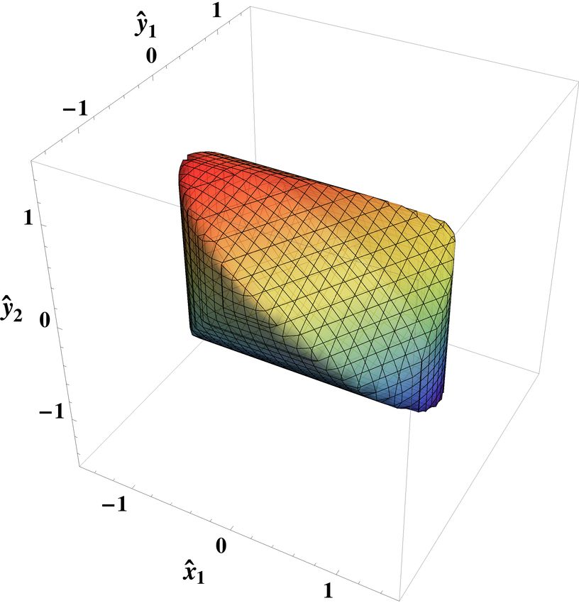
2) The mass of the object is sufficiently small that three                             S(x̃i , ỹi , z̃i ) is an algebraic function of the positions of the
      robots are able to lift the object.                                                 quadrotors. In order to satisfy (3), qi must satisfy the three
   3) The payload does not flip during manipulation, restrict-                            algebraic conditions:
      ing the orientation to |α| < π2 and |β| < π2 .
                                                                                                                  S(x̃i , ỹi , z̃i )T g̃ = 0.                  (5)
   4) We require the robots to assume positions that are on
      one side of the plane of the three pivot points.                                    The inverse problem reduces to the problem of solving for
   For the analysis, we will use a local frame, B, attached                               the three-dimensional set Qc ⊂ Q by solving for the nine
to the payload that is defined with the origin at P1 , the x                              variables {(x̃i , ỹi , z̃i ), i = 1, 2, 3} subject to (4, 5).
axis pointing toward P2 and the x − y plane coincident with                                   We now restrict our attention to a reduced space of pos-
the plane formed by P1 , P2 , and P3 . In this local coordinate                           sible configurations based upon the assumptions (3, 4). We
system, the components are denoted by (˜·) and given as:                                  introduce the notion of normalized components, denoted by
                                                                                          (ˆ·), with q̂i = [x̂i , ŷi , 1] to define the position of the ith robot
P1 = [0, 0, 0]T ,             P2 = [x̃p2 , 0, 0]T ,         P3 = [x̃p3 , ỹ3p , 0]T ;
                                                                                          projected to a constant height z̃i = 1 above the payload. Based
q̃1 = [x̃1 , ỹ1 , z̃1 ]T ,   q̃2 = [x̃2 , ỹ2 , z̃2 ]T ,   q̃3 = [x̃3 , ỹ3 , z̃3 ]T .   on this simplification (we now only need to solve for three
Note that without loss of generality, we assume that x̃P      P
                                                       2 > x̃3 ,
                                                                                          planar positions), we redefine the static equilibrium condition
restricting the possible permutations of Pi . Equation (2) takes                          as
the form:                                                                                                              S(x̂i , ŷi , 1)T g̃ = 0.               (6)
                          W̃λ = −g̃,                         (3)                          Solving the system of equations in (6) yields algebraic solu-
with                                                                                      tions for {x̂2 , x̂3 , ŷ3 } as functions of {x̂1 , ŷ1 , ŷ2 }. Note that
                     x̃1    x̃2 − x̃p2        x̃3 − x̃p3                                  any solution to (6) is indeed a solution to (5) after a scaling
                                                             
                     ỹ1       ỹ2            ỹ3 − ỹ3p                                of cable tension values. Further, we may compute the position
                     z̃1
                    
                                z̃2                z̃3
                                                                                         of the robots q̃i given the normalized coordinates q̂i and the
               W̃ = 
                                                              
                    0                             p                                      kinematic constraint (4) as
                                 0               ỹ3 z̃3
                                                              
                                                              
                                  p                  p
                    0       −x̃2 z̃2           −x̃3 z̃3                                                                       q̂i
                                                             
                                                                                                                    q̃i = li          + Pi .
                       0      x̃p ỹ2     x̃p3 ỹ3 − ỹ3p x̃3                                                                  kq̂i k
                            2
                              1 p Rp e
                                            T
                                                               
                                                 3                                        By using q̂i as coordinates, we can obtain closed-form analytic
                            (x̃ + x̃ )
                  g̃ = −mg           2     3                                             solutions for the positions of all robots that respect the
                            1 (ỹ3p )  × RT e3  .
                                3
                                                               
                                                               
                                    3                                                     kinematic constraints and the condition for static equilibrium.
                                        0                                                    If q̃i are chosen to satisfy the equations of equilibrium (3),
                                                                                          the multipliers can be obtained by:
  III. M ECHANICS OF 3-D MANIPULATION WITH CABLES
A. Robot positions for desired payload pose                                                                            λ = −W̃† g̃,
   The first problem that must be solved is the analog to the                             where W̃† is the Moore-Penrose inverse of W̃. This allows
inverse kinematics problem in parallel manipulators:                                      us to check to see if the equilibrium pose yields tensions
                                                                                          that satisfy (non-negative) lower and upper bounds. Figure 3
Problem 1 (Inverse Problem). Given the desired payload
                                                                                          depicts a representation of the bounded and positive tension
position and orientation (1), find positions of the robots, qi ,
                                                                                          workspace for various configurations.
that satisfy the kinematics of the robots-cables-payload system
and the equations of equilibrium (3).                                                     B. The pose of the payload for hovering robots
  The inverse kinematics problem is underconstrained. If the                              Problem 2 (Direct Problem). Given the actual positions
cables are in tension, we know that the following constraints                             of the robots, {q1 , q2 , q3 }, find the payload position(s) and
must be true:                                                                             orientation(s) satisfying the kinematics of the robots-cables-
                                                                                          payload system (4) and the equations of equilibrium (3).
             (x̃i − x̃pi )2 + (ỹi − ỹip )2 + (z̃i − z̃ip )2 = li2 ,             (4)
                                                                                             With hovering robots and cables in tension, we can treat
for i = {1, 2, 3}. We impose the three equations of static
                                                                                          the object as being attached to three stationary points through
equilibrium (3) to further constrain the solutions to the inverse
                                                                                          rigid rods and ball joints to arrive at the constraints in (4).
problem. This further reduces the degrees of freedom to three.
                                                                                          Accordingly the object has three degrees of freedom. Imposing
Finally, we require that there exist a positive, 3 × 1 vector of
                                                                                          the three equilibrium conditions in (5) we can, in principle,
multipliers, λ, that satisfies (3).
                                                                                          determine a finite number of solutions for this analog of the
   We solve this problem by finding the three screws (twists)
                                                                                          direct kinematics problem. While this theoretical setting allows
that are reciprocal to the three zero pitch wrenches. Define the
                                                                                          the analysis of the number of solutions using basic tools in
6 × 3 matrix S of twists with three linearly independent twists
                                                                                          algebraic geometry, very little can be established when the
such that the vectors belong to the null space of W̃T :
                                                                                          idealization of rigid rods is relaxed to include limits on cable
                                   W̃T S = 0.                                             tensions. Therefore we pursue a numerical approach to the
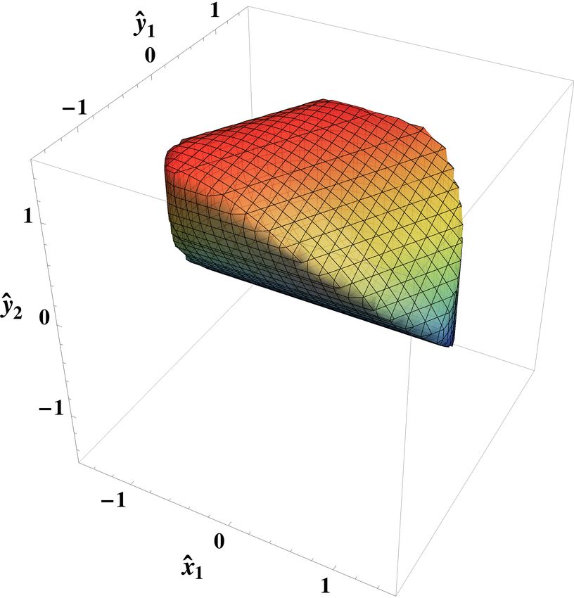
Cooperative Manipulation and Transportation with Aerial Robots
φ1
                                                                                        q1                      q3
                                                                                             θ1                       q2
                                                                                                          P3
                                                                                               P1              P2
                                                                                    W

                                                                       1                            (a)                                    (b)
       (a) α = β = 0, λ > 0                (b) α = β = 0, 0 < λ <      2
                                                                         mg
                                                                                   Fig. 4.     Determining the pose of the payload for hovering robots via
                                                                                   spherical coordinates (Fig. 4(a)). Given a representative robot configuration,
                                                                                   five equilibrium solutions for the pose of the payload are found via the
                                                                                   methods in Sect. III-B (Fig. 4(b)). The only stable configuration is orange
                                                                                   (as noted in Table I).

                                                                                   the height of the payload zC as the center of mass, which we
                                                                                   assume corresponds to the geometric center of the payload.
                                                                                   Therefore,
                                                                                                             3
                                                                                                          1X
                                                                                                    zC =        (zi + li cos φi ) ,          (7)
                                                                                                          3 i=1
                                                                                   where φi is defined in terms of spherical coordinates as
                                 1                                      1
(c) α = 0.3, β = 0, 0 < λ <      2
                                   mg     (d) α = β = 0.3, 0 < λ <      2
                                                                          mg       depicted in Fig. 4(a). From (7), we may derive the potential
                                                                                   energy of the payload as
Fig. 3. For a payload with mass m = 0.25 kg and x̃p2 = 1 m, x̃p3 = 0.5 m,                                                3
and ỹ3p = 0.87 m, the numerically determined workspace of valid tensions in                                         mg X
the normalized coordinates space {x̂1 , ŷ1 , ŷ2 }. Any point selected in these                  V = mgzC =                (zi + li cos φi ) ,              (8)
                                                                                                                      3 i=1
valid regions meets the conditions of static equilibrium while ensuring positive
and bounded tensions for all robots. Note that in these plots we do not consider
inter-robot collisions (as compared to Fig. 9(a)).
                                                                                   where m is the mass of the payload and g is acceleration due
                                                                                   to gravity. To study the stability of the payload, we consider
                             λ1           λ2       λ3                              the second-order changes of the potential energy. We first
                       1    0.06         0.80     5.48                             note that the robot-cables-payload system has three degrees of
                       2    −2.72        0.37     1.57
                                                                                   freedom when requiring that cables be in tension. Therefore,
                       3    −3.11        0.03     2.56
                       4    −2.64        0.27     7.50                             we choose to parameterize the solution of the potential energy
                       5    −5.54       −1.19    −0.61                             with respect to {φ1 , θ1 , φ2 } and define the Hessian of (8) as
                                                                                                                      ∂ V        ∂ V         ∂ V
                                                                                                               2           2        2
                                                                                                                                         
                               TABLE I
                                                                                                                                ∂φ1 ∂θ1     ∂φ1 ∂φ2
                                                                                                                  ∂∂φ
                                                                                                                           2
       E IGENVALUES , λi , OF (9) DEFINED BY THE EQUILIBRIUM                                                            1
                                                                                                                      2
                                                                                                                        V        ∂2V         ∂2V 
                                                                                             H (φ1 , θ1 , φ2 ) =                           ∂θ1 ∂φ2  .
                                                                                                                                                    
   CONFIGURATIONS FOR THE REPRESENTATIVE EXAMPLE (F IG . 4( B )).                                                                                            (9)
                                                                                                                  ∂θ12∂φ1       ∂θ12
                                                                                                                      ∂ V        ∂2V         ∂2V
problem by considering an alternative formulation. To numer-                                                         ∂φ2 ∂φ1    ∂φ2 ∂θ1      ∂φ22
ically solve the direct problem, we formulate an optimization                      Due to space constraints, we defer the presentation of the
problem which seeks to minimize potential energy of the                            analytic derivation of the entries of (9) to [10] where we
payload for a given robot configuration and payload geometry:                      show that a closed-form analytic representation of (9) is
      arg min         mgzC                                                         possible, enabling stability analysis of robots-cables-payload
          pi                                                                       configurations. In Fig. 4(b), we provide the resulting set of
               s.t.   kpi − qi k ≤ li , i = {1, 2, 3}                              equilibrium solutions to the direct problem for a representative
                                                                                   example robot configuration and the corresponding numerical
                      kpi − pj k = Lij , i, j = {1, 2, 3}, i 6= j
                                                                                   stability analysis in Table I.
where the objective function is linear in terms of pi (assuming
                                                                                                           IV. E XPERIMENTATION
a planar payload), and Lij is the metric distance between two
anchor points pi and pj .                                                          A. The quadrotor robots
                                                                                     In Sect. II, we assume point-model aerial robots but in
C. Stability analysis                                                              Sect. V provide results on a team of commercially available
   Assuming that each robot, qi , remains stationary, we wish to                   quadrotors (see Fig. 5). In this section we develop a transfor-
find the change in the potential energy of the payload. Define                     mation from desired applied forces to control inputs required
Cooperative Manipulation and Transportation with Aerial Robots
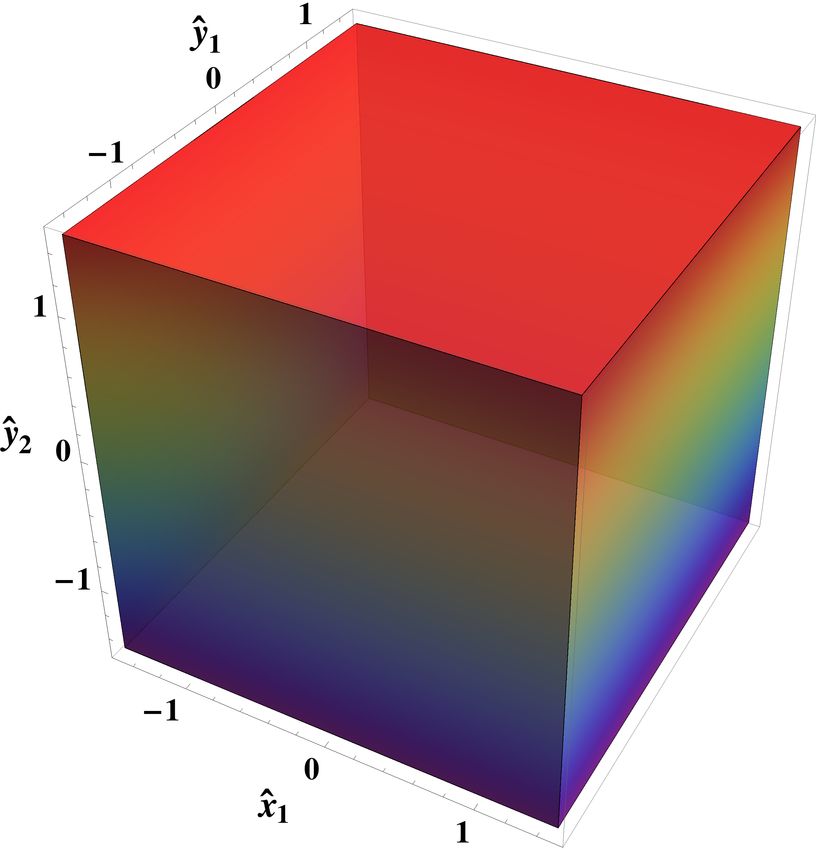
control inputs ν in the body-frame described in Sect. IV-A.
                                                                          The dynamics of the point robot in the world frame can be
                                                                          written as:
                                                                                                             Fx
                                                                                                             

                                                                                              mI3 q̈ = Fg + Fy  .              (11)
                                                                                                             Fz
                                                                          where Fx , Fy , and Fz are the control input forces in the world
                                                                          frame and Fg is the force due to gravity. These can be related
Fig. 5. The aerial robots and manipulation payload for experimentation.
                                                                          to the forces in the robot body frame:
The payload is defined by m = 0.25 kg and x̃p2 = 1 m, x̃p3 = 0.5 m, and                      0                      Fx
                                                                                                                  
ỹ3p = 0.87 m, with li = 1 m.                                                               0  = R(α, β, γ)−1 Fy  .               (12)
                                                                                            fz                      Fz
by the hardware platform. Some of this discussion is specific
to the quadrotor used for our experiments.                                Thus, for a given (current) γ, there is a direct relationship
   1) Model: We begin by considering an aerial robot in R3                between the triples (α, β, fz ) and (Fx , Fy , Fz ). Solving (12)
with mass m and position and orientation, q = [x, y, z] ∈ R3 ,            results in sixteen solutions for (α, β, fz ), eight of which
and R(α, β, γ) ∈ SO(3), respectively. We do not have direct               require fz ≤ 0. Requiring that the robot always apply thrust
access to the six control inputs for linear and angular force             with Fz > 0 reduces the solution set to the following:
control, but instead have access to four control inputs ν =
                                                                                 q
                                                                           fz = Fx2 + Fy2 + Fz2
[ν1 , . . . , ν4 ] defined over the intervals [ν1 , ν2 , ν3 ] ∈ [−1, 1]                  √ 
for the orientations and ν4 ∈ [0, 1] for the vertical thrust.                                 αn
                                                                            α = ± cos −1
                                                                                           √
   Based on system identification and hardware documenta-                                    2fz
                                                                          αn = Fx2 + 2Fx Fy sin(2γ) + Fy2 + 2Fz2 + Fx2 − Fy2 cos(2γ)
                                                                                                                                   
tion, we arrive at the following dynamic model relating the
control inputs and the forces and moments produced by the                                                                       !
                                                                                                            Fz
rotors in the body frame:                                                   β = ± cos −1
                                                                                                                                   .
                                                                                              Fz2 + (Fx cos(γ) + Fy sin(γ))2
                                                                                           p
                     q         q
              τx = −Kv,x α̇ − Kp,x (α − ν1 αmax )                                                                                      (13)
                     q         q
              τy = −Kv,y β̇ − Kp,y (β − ν2 βmax )                            From (13), it is clear that two solution sets are valid,
                     q         q
              τz = −Kv,z γ̇ − Kp,z ν3 γinc                                but only for specific intervals. For example, consider
              fz = ν4 fmax                                                pitch (β) when applying controls in the yaw directions
                                                                          [−π/2, 0, π/2, π] with {Fx , Fy , Fz } > 0. For each of the
where τx , τy , and τz are the torques along the body-fixed x,            four cases respectively, we expect β < 0, β > 0, β > 0, and
y, and z axes, respectively, and fz is the force (thrust) along           β < 0. A similar argument may be made for α. Therefore,
the body-fixed z axis.                                                    we must construct a piecewise-smooth curve as a function
   The relevant parameters above are defined as:                          of the external forces {Fx , Fy } and γ over the intervals
        q    q
   • Kp , Kv — feedback gains applied by the aerial robot;                [−π, γ1 ], [γ1 , γ2 ], [γ2 , π], defined by the zero points of the
   • fmax — maximum achievable thrust as a non-linear                     conditions in (13). For α, we find that
      function of battery voltage;
                                                                                                            Fx
                                                                                                           
   • αmax , βmax — maximum achievable roll and pitch an-                       [γα1 , γα2 ] = − tan    −1
                                                                                                            Fy
      gles;                                                                                    (                             
   • γinc — conversion parameter between the units of ν3 and                                       − 2 , − π2
                                                                                                      3π
                                                                                                                 if − tan−1 F      > π2
                                                                                                                               x
                                                                                            +       π π                     Fy
      radians.                                                                                      −2, 2               otherwise
All of these parameters were identified through system identi-
                                                                          In a similar manner, we find for β
fication. Therefore, in the discussion that follows, we consider                                    s               !
the following desired inputs:                                                                             Fx2    Fx
                                                                          [γβ1 , γβ2 ] = 2 tan −1
                                                                                                       1+ 2 −
                 d
                  α
                                        
                                         αmax
                                                                                                         Fy     Fy
                β d  
                 d  = ν1 ν2 ν3 ν4  βmax  ,                                                                             F2
                                                                                         (                        q                  
                                                                                                                                  Fx
                                                                                            − 3π ,   π
                                                                                                            tan −1
                                                                                                                      1 + Fx2 −            >   π
                                                                                                    
                                                            (10)                                   −     if
                γ                      γinc                                        +       2
                                                                                             π π   2                      y     Fy           4

                  fzd                     fmax                                               −2, 2                   otherwise
                                                                             We now construct piecewise-smooth solutions that reflect
noting that we can compute the control inputs ν given the
                                                                          the expected inputs for all values of γ. From (13), we denote
desired values assuming the parameters are known.
                                                                          the positive α solution as α+ and the negative solution as α− .
B. Controllers                                                            The piecewise-smooth input for α is
                                                                                                {α+ , α− , α+ } if Fy > 0
                                                                                             
   We now derive a transformation from the control inputs
                                                                                        α=
for our point-model abstraction in the world frame to the                                       {α− , α+ , α− } otherwise
Cooperative Manipulation and Transportation with Aerial Robots
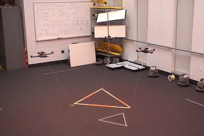
In a similar manner, for β we find

                    {β− , β+ , β− }     if Fx > 0
                  
              β=
                    {β+ , β− , β+ }     otherwise

   Both α and β become singular when Fy = 0. However, it
is clear from the definitions in (13) that at this singularity for
the intervals [−π, 0] and [0, π],

                        {α− , α+ } if Fx > 0
                      
                                                                                             (a)                                    (b)
                 α=
                        {α+ , α− } otherwise                                                                  Platform Error
                                                                                  1

and for the intervals [−π, −π/2], [−π/2, π/2], and [π/2, π]

                                                                      m2
                                                                               0.5

                                                                                  0
                                                                                   45   50         55   60         65          70     75   80      85

                     {β− , β+ , β− } if Fx > 0
                   
                                                                                  1
              β=
                     {β+ , β− , β+ } otherwise

                                                                      rad2
                                                                               0.5

                                                                                  0
                                                                                   45   50         55   60         65          70     75   80      85
                                                                                                                Time (s)
Of course, there remains the trivial solution of α = β = 0
                                                                                                             (c)
when Fx = Fy = 0.
   Therefore, we may define a force F = [Fx , Fy , Fz ] T in the                1
                                                                                                             Robot Positions

                                                                       x (m)
                                                                                0
world frame that is transformed into appropriate control inputs                −1
                                                                               −2
via (10, 12). To this end, we compute F in implementation                       2
                                                                                 45     50         55   60         65          70     75   80      85

                                                                       y (m)
                                                                                1
based on proportional-integral-derivative (PID) feedback con-                   0
                                                                               −1
trol laws determined by the desired robot configurations with                    45     50         55   60         65          70     75   80      85

                                                                                  2
                                                                          z (m)

feedforward compensation based on (11). For the purposes of                       1

this work, we additionally control ν3 to drive γ to zero.                         45    50         55   60         65
                                                                                                                Time (s)
                                                                                                                               70     75   80      85

   As a limitation of this approach, we note that the controller                                             (d)
above results in thrust fz for any desired input. Therefore,
when the robot is hovering at a level pose (α = β = 0), a            Fig. 6. In Fig. 6(a) the robots assume the desired configuration while in
desired horizontal motion for which Fx must be nonzero and           Fig. 6(b) one robot has suffered a large actuation failure. Figure 6(c) depicts
Fz = mg, results in an unintended vertical thrust fz > mg            the mean squared position and orientation error of the payload while Fig. 6(d)
                                                                     provides data on the individual robot control error. Vertical dashed lines in
until the robot rotates from the level pose.                         Figs. 6(c) and 6(d) show the exact time of the robot actuator failure.

C. Payload model                                                                                        V. R ESULTS
   The payload is a rigid frame with cable attachment points            Using the solution to the inverse problem presented in
given by x̃p2 = 1 m, x̃p3 = 0.5 m, and ỹ3p = 0.87 m with mass       Sect. III and the abstraction of a fully dynamic aerial vehicle to
m = 0.25 kg. The cable lengths are equal with li = 1 m.              a point robot in Sect. IV, we are able to experimentally verify
                                                                     our ability to lift, transport, and manipulate a six degree of
D. Simulation and Experiment Design                                  freedom payload by controlling multiple quadrotors.
   Our software and algorithms are developed in C/C++                A. Cooperative Lifting
using Player/Gazebo [11] and interfaced with MATLAB for                 We start with a symmetric configuration similar to that in
high-level configuration specification for both simulation and       Fig. 4(b) for benchmarking the performance of the system.
experiments.                                                         Figure 6(a) depicts the team of robots in this configuration
   Experiments are conducted with the AscTec Hummingbird             raising the payload to a specified pose in the workspace.
quadrotor [12] from Ascending Technologies GmbH with                 During the course of experimentation in this configuration, in
localization information being provided by a Vicon motion            one of the trials, a robot suffers a momentary actuator failure
capture system [13] running at 100 Hz with millimeter accu-          causing it to lose power and drop (see Fig. 6(b)). We use the
racy. Control commands are sent to each robot via Zigbee at          data from this trial to demonstrate the team’s ability to quickly
20 Hz. The quadrotor is specified to have a payload capacity         recover and return to the desired configuration. Analysis of the
of 0.2 kg with a physical dimension conservatively bound by          data in Figs. 6(c) and 6(d) suggests that the time constant for
a sphere of radius R = 0.3 m.                                        the closed loop response of the system is around 1 − 1.5 s.
   Robots can be positioned inside the 6.7 m × 4.4 m × 2.75 m
workspace with an error bound of approximately ±0.05 m               B. Cooperative manipulation and transport
in each direction. However, as the robots experience the                In this experiment, the system is tasked with manipulating
effects of unmodelled external loads and interactions during         the payload through a sequence of poses. For each pose, we
manipulation, errors increase to approximately ±0.15 m.              compute the desired configuration (q1 , q2 , q3 ) for the robots
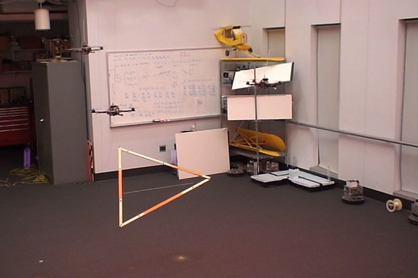
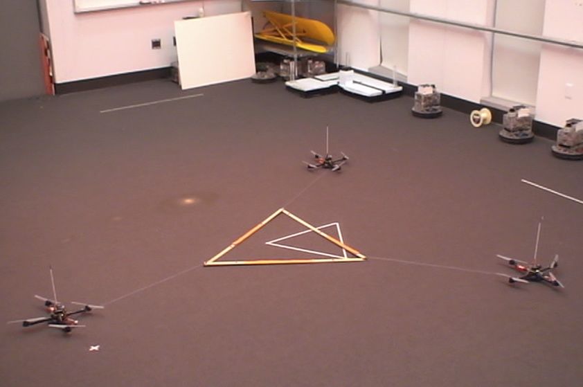
Cooperative Manipulation and Transportation with Aerial Robots
(a)                             (b)                            (c)                                                                 (d)                                     (e)

Fig. 7. Snapshots demonstrating cooperative manipulation and transportation. The team starts from initial conditions before takeoff (Fig. 7(a)), stabilizes the
platform at each desired pose (Figs.7(b) – 7(d)), and returns the payload to the first pose before landing (Fig. 7(e)). Colored circles highlight individual robot
positions during the evolution of the experiment. Videos of the experiments are available at http://kumar.cis.upenn.edu/movies/RSS2009.flv

                                                                                                                                                                Platform Pose
and drive each robot to the desired goal. The underlying con-                                                              1

                                                                                         X (m)
trol system avoids inter-robot collisions via a simple potential                                                         0.5
                                                                                                                           0

field controller derived from the point-robot model in (11)                                                                1
                                                                                                                               20   30   40   50         60       70          80     90   100    110   120   130

with each robot modeled as a sphere of radius R, guaranteeing

                                                                                         Y (m)
                                                                                                                         0.5
                                                                                                                           0

kqi −qj k > 2R for all pairs of robots. This results in a smooth,                                                              20   30   40   50         60       70          80     90   100    110   120   130

                                                                                                                           1

                                                                                         Z (m)
though unplanned, trajectory for the payload. Figures 7 and                                                              0.5
                                                                                                                           0
8 depict several snapshots during this experiment and the                                                                 50
                                                                                                                               20   30   40   50         60       70          80     90   100    110   120   130

                                                                                      Roll (deg)
resulting system performance, respectively.                                                                                0

                                                                                                                   −50
   This experiment demonstrates that even though the manipu-                                                                   20   30   40   50         60       70          80     90   100    110   120   130

                                                                                      Pitch (deg)
                                                                                                                          50

lation system is underactuated for n = 3, it is able to position                                                           0

                                                                                                                   −50
and orient the payload as commanded. The small oscillations                           Yaw (deg)                           50
                                                                                                                               20   30   40   50         60       70          80     90   100    110   120   130

around each equilibrium configuration are inevitable because                                                               0

                                                                                                                   −50
of the low damping and perturbations in the robot positions.                                                                   20   30   40   50         60       70
                                                                                                                                                                   Time (s)
                                                                                                                                                                            80       90   100    110   120   130

               VI. P LANNING M ULTI -ROBOT                                                                                                                      (a)
        M ANIPULATION AND T RANSPORTATION TASKS
                                                                                                                                                                 Platform Error

   In this section, we address motion planning for the aerial                                                              1
                                                                                          Position Error (m)

manipulation tasks and the generation of trajectories for the                                                            0.5

robots that respect (a) the kinematic workspace constraints;                                                               0
                                                                                                                               20   30   40   50         60       70          80     90   100    110   120   130
                                                                                               Orientation Error (deg)

(b) the conditions of stable equilibrium for the payload; (c)                                                            80

constraints on the cable tensions (λmax ≥ λi > 0); and                                                                   60
                                                                                                                         40
                                                                                                                         20
(d) the geometric constraints necessary to avoid collisions                                                                0
                                                                                                                               20   30   40   50         60       70         80      90   100    110   120   130
(kqi −qj k > 2R). In Sect. III, we computed Qc to to be the set                                                                                                     Time (s)

of robot positions satisfying (a, b) with positive tension in each                                                                                              (b)
cable. We now derive the effective workspace for the robots                                                                                                   Robot Control Errors

QM ⊂ Qc consisting of robot positions that satisfy (a-d)                                                                 0.5
                                                                                        x (m)

above. The planned trajectories of the robots must stay within                                                            0
                                                                                                                               20   30   40   50         60       70          80     90   100    110   120   130
QM which has a complex shape owing to the nonsmooth                                                                      0.5
                                                                                        y (m)

constraints in (a-d).                                                                                                     0
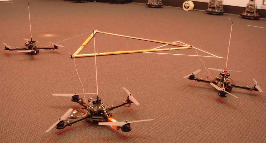
   Figure 9 illustrates the effective workspace QM parameter-                                                                  20   30   40   50         60       70          80     90   100    110   120   130

ized by (x̂1 , ŷ1 , ŷ2 ). Indeed for a given payload pose, there are
                                                                                                                         0.5
                                                                                        z (m)

multiple points in the workspace that satisfy the conditions of                                                           0
                                                                                                                               20   30   40   50         60       70
                                                                                                                                                                    Time (s)
                                                                                                                                                                             80      90   100    110   120   130

stable equilibrium. Three representative conditions are shown                                                                                                   (c)
in the figure. Thus during motion planning it is possible to
optimize any number of design goals, including equal sharing                         Fig. 8. Data from the manipulation and transportation experiment, including:
                                                                                     pose data for the payload overlaid with a dashed line representing desired
of loads by the cooperating robots, robustness to disturbances                       values (Fig. 8(a)), aggregate position and orientation error of the payload
to the payload, and maximizing the stability of the robots-                          (Fig. 8(b)), and individual robot control errors (Fig. 8(c)).
payload system. To demonstrate this, we consider the response
of the payload to an external disturbance in experimentation                         determined by the natural frequency-based measure attenuates
given two distinct robot configurations selected from the space                      the payload error more quickly than the other configuration in
of valid solutions QM depicted in Fig. 9(a). The first mirrors                       which the lower natural frequency results in oscillations that
the simulation configuration shown in Fig. 9(b) while the sec-                       take longer to damp out.
ond configuration is selected to maximize the smallest natural                          In future work we will further investigate the planning
frequency of the payload given by the smallest eigenvalue of                         of aerial manipulation by exploring the use of sample-based
the Hessian in (9). Figure 10 shows that the robot configuration                     planning methods for payload trajectory control. While the
Cooperative Manipulation and Transportation with Aerial Robots
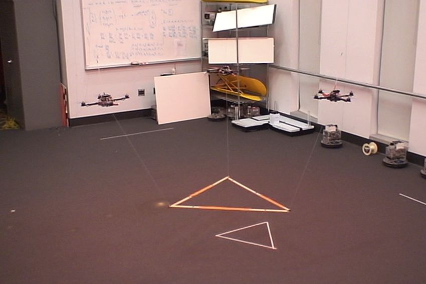
VII. C ONCLUSION AND F UTURE W ORK
                                                                                          We presented a novel approach to aerial manipulation and
                                                                                       transport using multiple aerial robots. We derived a mathe-
                                                                                       matical model that captures the kinematic constraints and the
                                                                                       mechanics underlying stable equilibria of the underactuated
                                                                                       system. The number of unconstrained degrees of freedom is
                                                                                       equal to six less the number of robots. We also presented
                 (a)                                       (b)                         an experimental implementation and results that suggest that
                                                                                       cooperative manipulation can be used as an effective way of
                                                                                       manipulating and transporting payloads that are beyond the
                                                                                       capability of individual micro UAVs.
                                                                                          The main limitation of our approach lies in our inability to
                                                                                       damp out oscillations in the underdamped system. Because
                                                                                       of this, our trajectory following capabilities are limited to
                                                                                       slow motions with harmonics well under the fundamental
                                                                                       frequencies of around 3 − 5 Hz. One possibility is to use the
                 (c)                                       (d)                         robots to actively damp out oscillations using methods anal-
                                                                                       ogous to controlling flexible manipulators. We are currently
Fig. 9. Various points in QM for α = β = 0 (Figs. 9(b)–9(d)). Figure 9(a)              engaged in a more thorough study of the underlying joint
depicts numerically determined regions of valid tensions in the space of q̂            configuration space and the effects of cable constraints with a
requiring λi < 12 mg and kqi − qj k > 1 m (for collision avoidance), with              view to developing motion planning algorithms. We are also
black points indicating the configurations selected in Figs. 9(b)-9(d). For
completeness, the normalized coordinates, {x̂1 , ŷ1 , ŷ2 }, of each configu-         considering the application of control and estimation methods
ration follows: {−0.2724, −0.3054, −0.3054} (Fig. 9(b)), {0, 0, −0.9}                  that relax our current reliance on globally available state
(Fig. 9(c)), {0.6, 0.45, −0.9} (Fig. 9(d)).                                            information and enable a better understanding of the effects
                                                                                       of sensing and actuation uncertainty on control performance.
 Error HmL
  0.6
  0.3                                                                                                                 R EFERENCES
    0                                                                       Time HsL
     50             55               60               65               70               [1] R. M. Murray, “Trajectory generation for a towed cable system using
                                      (a)                                                   differential flatness,” in IFAC World Congress, San Francisco, CA, July
                                                                                            1996.
 Error HmL                                                                              [2] P. Cheng, J. Fink, S. Kim, and V. Kumar, “Cooperative towing with
  0.8                                                                                       multiple robots,” in Proc. of the Int. Workshop on the Algorithmic
  0.4
    0                                                                       Time HsL
                                                                                            Foundations of Robotics, Guanajuato, Mexico, Dec. 2008.
     50             55               60               65               70               [3] E. Stump and V. Kumar, “Workspaces of cable-actuated parallel ma-
                                                                                            nipulators,” ASME Journal of Mechanical Design, vol. 128, no. 1, pp.
                                      (b)
                                                                                            159–167, Jan. 2006.
Fig. 10. A disturbance is applied to the payload in experimentation at time             [4] R. Verhoeven, “Analysis of the workspace of tendon-based stewart plat-
55 s in two trials. In Fig. 10(a), the robot configuration is selected based on             forms,” Ph.D. dissertation, University Duisburg-Essen, Essen, Germany,
the maximization of the natural frequency of the payload and in Fig. 10(b),                 July 2004.
the robot configuration is chosen to be similar to that shown in Fig. 9(b).             [5] S. R. Oh and S. K. Agrawal, “A control lyapunov approach for feedback
Note that the configuration in Fig. 10(a) attenuates error more quickly.                    control of cable-suspended robots,” in Proc. of the IEEE Int. Conf. on
                                                                                            Robotics and Automation, Rome, Italy, Apr. 2007, pp. 4544–4549.
                                                                                        [6] P. Bosscher and I. Ebert-Uphoff, “Wrench-based analysis of cable-driven
analytic representation of our feasible workspace is compli-                                robots,” in Proc. of the IEEE Int. Conf. on Robotics and Automation,
cated, fast numerical verification suggests standard sample-                                vol. 5, New Orleans, LA, Apr. 2004, pp. 4950–4955.
                                                                                        [7] K. H. Hunt, Kinematic Geometry of Mechanisms. Oxford University
based methods can be used for this task. Additionally, while                                Press, 1978.
it is possible that the workspace of configurations with tension                        [8] J. Phillips, Freedom in Machinery. Cambridge University Press, 1990,
limits is not simply connected, in our extensive numerical                                  vol. 1.
                                                                                        [9] J. M. Selig, Geometric Fundamentals of Robotics. Springer, 2005.
studies, we have not found this to happen with realistic values                        [10] N. Michael, S. Kim, J. Fink, and V. Kumar, “Kinematics and statics of
of geometric parameters and tension bounds. This suggests                                   cooperative multi-robot aerial manipulation with cables,” University of
that it should be possible to transition smoothly from one                                  Pennsylvania, Philadelphia, PA, Tech. Rep., Mar. 2009, Available online
                                                                                            at http://www.seas.upenn.edu/∼nmichael.
configuration to another without loss of cable tension. Finally,                       [11] B. P. Gerkey, R. T. Vaughan, and A. Howard, “The Player/Stage Project:
the fact that the direct problem has multiple stable solutions                              Tools for multi-robot and distributed sensor systems,” in Proc. of the Int.
is a potential source of concern in real experimentation since                              Conf. on Advanced Robotics, Coimbra, Portugal, June 2003, pp. 317–
                                                                                            323.
positioning the robots at a desired set of positions does not                          [12] “Ascending Technologies, GmbH,” http://www.asctec.de.
guarantee that the payload is at the desired position and                              [13] “Vicon Motion Systems, Inc.” http://www.vicon.com.
orientation. In a forthcoming paper [14], we show that by                              [14] J. Fink, N. Michael, S. Kim, and V. Kumar, “Planning and control for
                                                                                            cooperative manipulation and transportation with aerial robots,” in Int.
further constraining QM , we can reduce the direct problem to                               Symposium of Robotics Research, Zurich, Switzerland, Aug. 2009, To
a Second Order Cone Program (SOCP). We plan to incorporate                                  Appear.
these constraints into our motion planning algorithm.
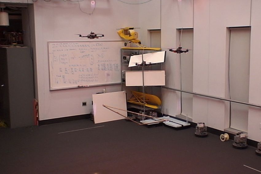
Cooperative Manipulation and Transportation with Aerial Robots Cooperative Manipulation and Transportation with Aerial Robots
You can also read