Inferring Temporal Order of Images From 3D Structure
←
→
Page content transcription
If your browser does not render page correctly, please read the page content below
Inferring Temporal Order of Images From 3D Structure

            Grant Schindler           Frank Dellaert                           Sing Bing Kang
                Georgia Institute of Technology                       Microsoft Research, Redmond, WA
              {schindler,dellaert}@cc.gatech.edu                          SingBing.Kang@microsoft.com

                         Abstract

    In this paper, we describe a technique to temporally sort
a collection of photos that span many years. By reasoning
about persistence of visible structures, we show how this
sorting task can be formulated as a constraint satisfaction
problem (CSP). Casting this problem as a CSP allows us to
efficiently find a suitable ordering of the images despite the
large size of the solution space (factorial in the number of
images) and the presence of occlusions. We present experi-
mental results for photographs of a city acquired over a one      Figure 1. Given an unordered collection of photographs, we infer
                                                                  the temporal ordering of the images by reasoning about the visi-
hundred year period.
                                                                  bility of 3D structure in each image.

                                                                  2. Related Work
1. Introduction
                                                                      SFM is now a well-studied problem, and the early stages
    Cameras and skyscrapers have now coexisted for more           of our approach proceed very much in the same manner
than a century, allowing us to observe the development of         as in [11], recovering calibrated cameras and the 3D point
cities over time. We are interested in being able to automat-     locations based on 2D correspondences between images.
ically construct a time-varying 3D model of a city from a         Time-varying SFM problems have been studied in the con-
large collection of historical images. Such a model would         text of ordered image-sequences of objects in motion [7],
reflect the changing skyline of the city, with buildings cre-     while we work with an unordered (both spatially and tempo-
ated, modified, and destroyed over time. It would also be         rally) collection of images. Although reasoning about vis-
useful to historians and urban planners both in organizing        ibility and occlusions has previously been applied to view
collections of thousands of images (spatially and tempo-          synthesis from multiple images [8], surface reconstruction
rally) and in generating novel views of historical scenes by      [13], and model-based self-occlusion for tracking [10], it
interacting with the time-varying model itself.                   has not been used in the context of temporal sorting.
    To extract time-varying 3D models of cities from histori-         The earliest work on temporal reasoning involved the
cal images, we must perform inference about the position of       development of an interval algebra describing the possi-
cameras and scene structure in both space and time. Tradi-        ble relationships between intervals of time [1]. A number
tional structure from motion (SFM) techniques can be used         of specific temporal reasoning schemes were later captured
to deal with the spatial problem, while here we focus on the      by temporal constraint networks [3] which pose the tem-
problem of inferring the temporal ordering for the images as      poral inference problem as a general constraint satisfaction
well as a range of dates for which each structural element        problem. Such networks are often used for task scheduling,
in the scene persists. We formulate this task as a constraint     given constraints on the duration and ordering of the tasks.
satisfaction problem (CSP) based on the visibility of struc-      Efficient solutions to temporal constraint networks rely on
tural elements in each image. By treating this problem as a       sparsity in the network, whereas our problem amounts to
CSP, we can efficiently find a suitable ordering of the im-       handling a fully connected network. Uncertainty was later
ages despite the large size of the solution space (factorial in   introduced into temporal constraint networks [4, 5, 2] by re-
the number of images) and the presence of occlusions.             laxing the requirement that all constraints be fully satisfied.
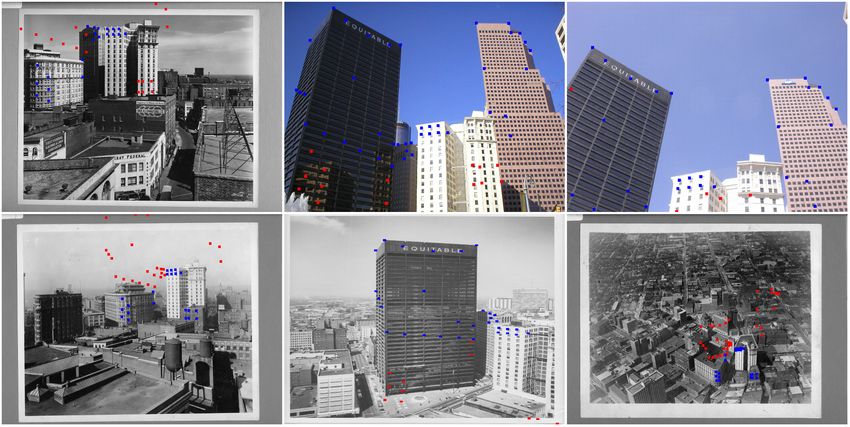
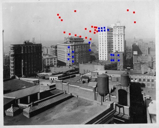
Figure 3. Point Classification. In each image, every 3D point is
                                                                      classified as observed (blue), missing (red), out of view (white)
                                                                      or occluded (white). The missing points belong to buildings that
                                                                      do not yet exist at the time the photograph was taken. Classi-
                                                                      fications across all images are assembled into a visibility matrix
                                                                      (right) which is used to infer temporal ordering. Each column of
                                                                      the visibility matrix represents a different image, while each row
                                                                      represents the visibility of a single 3D point across all images.

Figure 2. Overview of Approach. A fully automated system for          4. Visibility Reasoning
building a 4D model (3D + time) of a city from historical pho-
tographs would consist of all these steps. Here, we concentrate on       The problem we will address is inferring the temporal
the highlighted steps of visibility reasoning and constraint satis-   ordering of a set of n un-ordered images I1..n registered to
faction to infer a temporal ordering of images which can then be      a set of m 3D points X1..m . The key to inferring temporal
used to construct the 4D model.                                       order from a collection of historical urban images is that
                                                                      different sets of 3D structures exist in the same place in the
                                                                      world at different points in time. Thus, we must determine
                                                                      which structures exist in each image, and to do this we must
3. Overview of Approach                                               reason about the visibility of each 3D point in each image.
                                                                      We show here how to encode the information provided by
    We are interested in inferring the temporal ordering of           each image Ij about every 3D point Xi in a visibility matrix.
images as one step in a system for producing time-varying
3D models of cities from historical photographs. As sum-              4.1. Visibility Classification
marized in Figure 2 the process begins by performing fea-
ture detection and matching on a set of input photographs,               To determine whether a building exists at the time an
followed by SFM to recover 3D points and camera poses.                image was taken, we reason about the visibility of each 3D
The feature detection and SFM steps are beyond the scope              point on that building. Assuming known projection matri-
of this paper and we do not discuss them in detail here, other        ces P1..n for each of the n cameras C1..n corresponding to
than to say that in this work the feature detection and match-        images I1..n , every 3D point can be classified in each image
ing are performed manually, while SFM is automatic.                   as observed, missing, out of view, or occluded as fol-
                                                                      lows. If a measurement uij exists for point Xi in image
                                                                                                                                Ij,
   In this paper, we focus on the problems of visibility rea-                                                                  Xi
                                                                      the point is observed. If the projection xij = Pj
soning, temporal ordering, and time-varying 3D model con-                                                                      1
struction as highlighted in Figure 2. Our method takes 3D             of point Xi in image Ij falls outside the field of view of
points and camera poses as input and uses them to compute             the camera (as defined by the width and height of the cor-
a matrix describing the visibility of each 3D point in each           responding image), the corresponding point is classified as
image (Section 4). The temporal ordering of the images is             out of view for that image. If the projection xij is within
then recovered by reordering the columns of this visibility           the field of view of the camera but no measurement uij
matrix in a CSP framework (Section 5). Finally, the inferred          exists, the point may be classified either as missing or
temporal ordering is used to visualize a 4D model (space +            occluded, and further work is required to determine which
time) of the changing city (Section 6).                               classification is correct (see Section 4.2).
The intuition behind this classification is that we want to
know whether the physical structure corresponding to point
Xi existed at the time that image Ij was captured. If it does
not appear where we expect it to be, either it did not exist at
the time (missing) or else something is blocking our view
of it (occluded). We discuss how to distinguish between
these two cases in the next section.
(a) violates constraints
4.2. Occlusion
We can also use occlusion reasoning to determine why
a building might not appear in a given image. To this end,
we assume that the 3D points X1..m correspond to a sparse
(b) satisfies constraints (c) satisfies constraints
sampling of the surface of a number of solid structures in the
scene. For every triplet of points, the triangle Xa Xb Xc that Figure 4. Visibility constraints. The columns of the visibility ma-
they define may or may not lie along the surface of a solid trix must be reordered such that the situation in (a) never occurs
– it should never be the case that some structure is visible, then
structure. If we can find a triangulation of these points that
vanishes, then appears again. Rather, we expect that buildings are
approximates the solid structure, the faces of such a mesh constructed and exist for some amount of time before being de-
will occlude the same set of points occluded by the physical molished as in (b). Note that the constraint in (a) does not rule out
structure, and these occluding faces can be used to distin- the situation in (c) where structure becomes occluded.
guish between points that are missing and out of view.
Inspired by [6] and the image-consistent triangulation
method of [9], we proceed as follows: For each image See Figure 3 for an example of such a visibility matrix. In
Ij , we compute the Delaunay triangulation of the measure- all figures, the value +1 is indicated with a blue dot, −1
ments uij in that image. Each 3D triangle corresponding to with a red dot, and 0 with a white dot. Note that the columns
a face in the Delaunay triangulation is a potential occluder of such a matrix correspond to entire images, while the rows
and for each triangle, we test whether it fails to occlude any correspond to single 3D points.
observed points in the scene. That is, if a face is intersected
by a line segment Oj Xi from any camera’s center of pro- 5. Constraint Satisfaction Problem
jection Oj to any observed 3D point Xi corresponding to a
measurement uij , it is removed from the potential pool of We pose the temporal ordering problem as a constraint
occluders. The intuition behind this approach is that if the satisfaction problem (CSP), where constraints are applied
triangle was a true occluder, it would have blocked such a to the visibility matrix of the given scene. Specifically,
measurement from being observed. After testing all faces once a visibility matrix V is constructed, the temporal or-
against all observed points Xi in all images Ij , we are left dering task is transformed into the problem of rearranging
with a subset of triangles which have never failed to block the columns of V such that the visibility pattern of each
any 3D point from view, and we treat these as our occluders. point is consistent with our knowledge about how buildings
To determine whether a point Xi is missing or occluded are constructed. Our model assumes that every point Xi is
in a given image Ij , we construct a line segment from the associated with a building in the physical world, and that
center of projection Oj of camera Cj to the 3D point Xi . buildings are built at some point in time TA , exist for a fi-
If this line segment Oj Xi intersects any of the occluding nite amount of time, and may be demolished at time TB to
triangles, the point is classified as occluded. Otherwise the make way for other buildings. We also assume that build-
point is classified as missing, indicating that the point Xi ings are never demolished and then replaced with an iden-
did not exist at the time image Ij was captured. tical structure. These assumptions gives rise to constraints
on the patterns of values permitted on each row in V .
4.3. Visibility Matrix The constraints on the visibility matrix can be formalized
Finally, we can capture all this information in a conve- as follows: on any given row of V , a value of −1 may not
nient data structure—the visibility matrix. We construct an occur between any two +1 values. This corresponds to the
m × n visibility matrix V indicating the visibility of point expectation that we will never see a building appear, then
Xi in image Ij as disappear, then reappear again, unless due to occlusion or
being outside the field of view of the camera (see Figure
4). The valid image orderings are then all those that do not
+1 if Xi is observed in Ij
vij = −1 if Xi is missing in Ij violate this single constraint.
0 if Xi is out of view or occluded in Ij Because we have expressed the temporal ordering prob-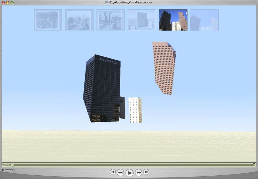
Figure 5. Local Search starts from a random ordering and swaps columns and groups of columns in order to incrementally decrease the
number of constraints violated. Here, 30 images are ordered by taking only 10 local steps.

lem in terms of constraints on the visibility matrix, we            5.2. Properties of Ordering Solutions
can use the general machinery of CSPs to find a solution.
                                                                       Solving the above constraint satisfaction problem may
A common approach to CSPs is to use a recursive back-
                                                                    give us more than just one possible temporal ordering of the
tracking procedure which explores solutions in a depth first
                                                                    images. For the n images, there may be r eras in which
search order by assigning an image Ij to position 1, then
                                                                    different combinations of structures coexist. If r < n, there
another image to position 2, etc. At each step, the partial so-
                                                                    is more than one solution to the constraint satisfaction prob-
lution is checked and if any constraints are violated, the cur-
                                                                    lem. In particular, any two images captured during the same
rent branch of search is pruned and the method “backtracks”
                                                                    era may be swapped in the ordering without inducing any
up one level to continue the search, having just eliminated
                                                                    constraint violations in the visibility matrix.
a large chunk of the search space. Given that our problem
                                                                       In addition, there is a second class of solutions for which
has n! solutions (i.e., factorial in the number of images n),
                                                                    time is reversed. This is because any ordering of the
this method becomes computationally intractable for even
                                                                    columns that satisfies all constraints will still satisfy all con-
relatively small numbers of images.
                                                                    straints if the order of the columns is reversed. In practice,
                                                                    one can ensure that time flows in the same direction for all
5.1. Local Search                                                   solutions by arbitrarily specifying an image that should al-
                                                                    ways appear in the first half of the ordering. This is anal-
   CSPs can also be solved using a local search method to           ogous to the common technique of fixing a camera at the
get closer and closer to the solution by starting at a random       origin during structure from motion estimation.
configuration and making small moves, always reducing the
number of constraints violated along the way. This solution         5.3. Dealing with Uncertainty
has been famously applied to solve the n-queens problem
for 3 million queens in less than 60 seconds [12].                     The above formulation depends upon an explicit decision
                                                                    as to the visibility status of each point in each image, and
   For our problem, a local search is initialized with a ran-
                                                                    cannot deal with misclassified points in the visibility matrix.
dom ordering of the images, corresponding to a random or-
                                                                    For example, if a point is not observed in an image, it is
dering of the columns in the visibility matrix V . At each
                                                                    crucial that the point receives the correct label indicating
step of the search, all local moves are evaluated. In our
                                                                    whether the point no longer existed at the time the image
case, these local moves amount to swapping the position of
                                                                    was taken, or whether it was simply occluded by another
two images or of two groups of images by rearranging the
                                                                    building. If a single point is misclassified in one image,
columns of the matrix V accordingly. In practice, swapping
                                                                    it may cause all possible orderings to violate at least one
larger groups of images allows solutions to be found more
                                                                    constraint, and the search will never return a result.
quickly, preserving the progress of the search by keeping
                                                                       The ideal case, in which there are no occlusions and no
constraint-satisfying sub-sequences of images together.
                                                                    points are out of view, will rarely occur in practice and there
   During local search, we consider a number of candidate           are a number of ways a point might be misclassified:
orderings of the columns of the visibility matrix, where dif-
ferent arrangements of columns will violate different num-             • Points that really should have been observed might,
bers of constraints. As described above, a constraint is vio-            due to failure at any point during automated feature
lated if, on a given row, a point is classified as missing be-           detection or due to missing or damaged regions of his-
tween two columns in which it was observed. The best lo-                 torical images, be classified as missing.
cal move is then the move that results in the ordering that vi-
olates the fewest constraints of all the candidate local moves         • Points that were occluded by un-modeled objects
being considered. If there is no move which decreases the                (such as trees or fog) may falsely be labeled missing.
number of constraints violated, we reinitialize the search             • Points that were really occluded may fail to be blocked
with a random ordering and iterate until a solution is found.            by occlusion geometry due to errors in SFM estima-
Once an ordering of the columns is found that violates no                tion, and instead be falsely labeled as missing.
constraints, the temporal ordering of the images is exactly
the ordering of the columns of the visibility matrix. Figure           • Points that are truly missing may be falsely explained
5 demonstrates the progress of such a local search.                      away as occluded.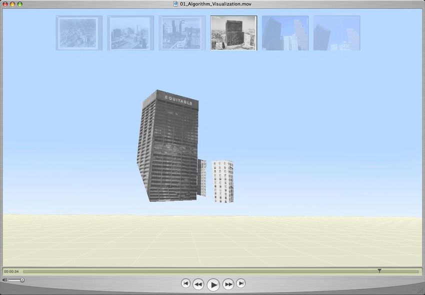
In practice, some combination of all these errors may occur.
   We achieve robustness to misclassified points without in-
troducing any additional machinery. CSPs can implicitly
cope with this kind of uncertainty by relaxing the require-
ment that all constraints be satisfied. We modify the local
search algorithm to return the ordering that satisfies more
constraints than any other after a fixed amount of searching.
Under such an approach, we can no longer be absolutely
certain that the returned solution is valid, but we gain the               (a)    (b)    (c)                  (d)
ability to apply the approach to real-world situations.
                                                                   Figure 6. Structure Segmentation. Beginning from a random
                                                                   ordering of the visibility matrix (a), local search re-orders the
5.4. Structure Segmentation                                        columns to the correct temporal ordering (b), and then rows are re-
    In order to build a convincing 3D model of a city, we          ordered to group 3D points that appear and disappear at the same
                                                                   times (c). We compute 3D convex hulls of each group of points to
need to segment the 3D point cloud that results from SFM
                                                                   get solid geometrical representations of buildings in the scene (d).
into a set of solid structures. In fact, we can use the visibil-
ity matrix V to extract such a building segmentation directly
from the recovered image ordering. Once the columns have
been reordered using local search, similar visibility patterns         In our second experiment, we deal with a more difficult
become apparent across the rows of the matrix. This is due         group of 20 images of a scene consisting of 92 3D points
to the fact that multiple 3D points originate from the same        (Figure 8). These images contain a number of misclassified
physical structures in the world, and thus come in and out         points due to occlusions by trees and un-modeled buildings,
of existence at the same time. This is made more appar-            as well as errors in the estimation of 3D point locations and
ent by reordering the rows of the visibility matrix to group       camera positions by SFM. As such, we do not expect to find
points that share times of appearance TA and disappearance         an ordering that satisfies all constraints, so we instead use
TB . Such a reordering amounts to segmenting the 3D point          1000 iterations of local search to find the ordering which
cloud into disjoint sets. By taking the 3D convex hull of          violates the fewest constraints. For each iteration of local
each cluster of points, we get approximate scene geometry          search, we begin from a new random ordering of the im-
which can be textured and used for further synthesis of new        ages. Note the number of iterations of search (1000) is con-
views in space and time (see Figure 6).                            siderably smaller than the number of possible orderings, in
                                                                   this case 20! ≈ 2.4 × 10¹⁸ . This local search returns an
                                                                   ordering (Figure 8) for which constraints are violated on 15
6. Results                                                         of the 92 rows of the visibility matrix. In the absence of any
    We tested our method on a set of images of a city col-         ground truth dates for the images, and with no exact solu-
lected over the period from 1897 to 2006. For the results          tion to the CSP in this case, it can be difficult to evaluate the
presented here, feature detection and matching were per-           quality of the returned ordering. However, despite the large
formed manually. Given a set of 2D correspondences across          number of constraints violated, the ordering returned is con-
images, the remaining steps of the algorithm beginning with        sistent both with the sets of buildings which appear in each
SFM (see Figure 2) are performed automatically.                    image and with the known dates of construction and demo-
    In our first experiment, we find a temporal ordering for       lition for all modeled buildings in the scene. The ordered
6 images of a scene containing 56 3D points (Figure 7). In         visibility matrix for this experiment is shown in Figure 9.
this case, we purposely chose photographs with clear views            In our third experiment, to simulate a larger problem, we
of all structure points, meaning that none of the points are       synthesize a scene containing 484 randomly distributed 3D
misclassified in the visibility matrix and an exact solution       points and 30 cameras placed in a circle around the points.
to the ordering is guaranteed. Due to the small number of          Each point is assigned a random date of appearance and dis-
images, we perform an exhaustive back-tracking search to           appearance, while each camera is assigned a single random
find all possible ordering solutions. Back-tracking search         date at which it captures an image of the scene. The result-
finds that out of the 6! = 720 possible orderings, there are       ing synthetic images only show the 3D points that existed
24 orderings which satisfy all constraints, one of which is        on the date assigned to the corresponding camera. The size
shown in Figure 7. The 24 solutions are all small variations       of the solution space (30! = 2.65 × 1032 ) necessitates local
of the same ordering—images 1 and 2 may be interchanged,           search for this problem. Starting from a random ordering,
as may images 4, 5, and 6, and finally the entire sequence         a solution that violates no constraints is found just 26 lo-
may be reversed such that time runs backwards. For this            cal moves away from the random initialization, taking less
small problem, the search takes less than one second.              than one minute of computation. In contrast to the previous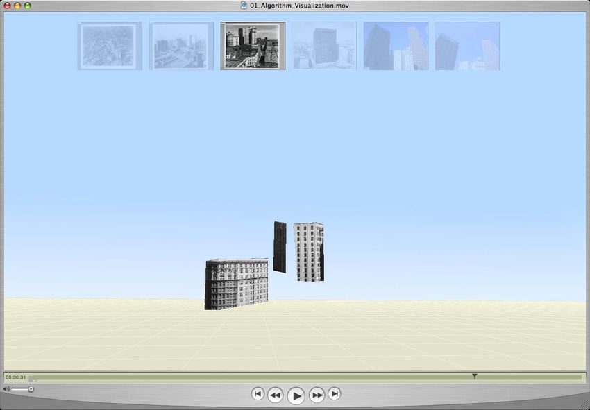
Figure 7. Inferred temporal ordering of 6 images. In the case where there are no occlusions of observed points, we can guarantee that
a solution exists that violates no constraints. The ordering shown is one of 24 orderings that satisfy all constraints. The other solutions
involve swapping sets of images that depict the same set of structures and reversing the direction of time.

Figure 8. Inferred ordering of 20 images. Despite many misclassified points, the presence of un-modeled occlusions such as trees, and a
solution space factorial in the number of images (20! ≈ 2.4 × 10¹⁸ ), an ordering consistent with the sets of visible buildings is found by
using local search to find the ordering that violates the fewest constraints. In such a case, there is no single solution which satisfies all
constraints simultaneously.

experiment, a solution is quickly found for this synthetic
scene (without the need to reinitialize the search) because
no points are misclassified for the synthesized images.
   Finally, we use the structure segmentation technique de-
scribed in Section 5.4 to automatically create a time-varying
3D model from the 6 images in Figure 7. After ordering
the columns of the visibility matrix to determine temporal
order, we reorder the rows to group points with the same
dates of appearance and disappearance. We then compute
the convex hulls of these points and automatically texture
                                                                         Figure 9. Ordered visibility matrices for sets of 6 images (left) and
the resulting geometry to visualize the entire scene (see Fig-
                                                                         20 images (right). The ordering of the 6 images on the left was
ure 10). Textures are computed by projecting the triangles               found with backtracking search and satisfies all constraints. The
of the geometry into each of the 6 images and warping the                ordering of the 20 images on the right violates the fewest con-
corresponding image regions back onto the 3D geometry.                   straints of all solutions found with 1000 iterations of local search.
                                                                         In the latter case, misclassified points caused by un-modeled oc-
7. Discussion                                                            clusions lead to a situation in which no ordering can simultane-
                                                                         ously satisfy all constraints.
    The computation time required for local search depends
upon several factors. The main computational cost is com-
puting the number of constraints violated by a given order-
ing of the visibility matrix, which increases linearly with m            the true solution using only local moves.
the number of points in the scene and n the number of im-                    Finally, note that the nature of the dates we infer for
ages being ordered. In addition, at each step of local search,           scene structure is abstract. For example, consider the build-
the number of tested orderings increases with n2 since there             ing depicted in the first image in Figure 8. Rather than in-
are (n)(n−1)
         2     ways to select two images to be swapped.                  ferring that this building existed from 1902 to 1966, we can
    As demonstrated in the above experiments, the amount                 only infer that it existed from the time of Image 1 to the
of computation also varies inversely with the number of                  time of Image 13 (where images are numbered by their po-
valid orderings for a given visibility matrix. For ordering              sition in the inferred temporal ordering). Without additional
problems that admit many solutions, the random initializa-               knowledge, this is the most we can confidently say about
tion of local search will often be close to some valid order-            when the building existed. When a human inspects a histori-
ing, and will thus solve the problem quickly. This is, in                cal photograph, he or she may assign a time to it by identify-
fact, the key to the success of local search on the n-queens             ing objects in the scene with known dates of existence—this
problem of [12], where the number of solutions actually in-              may include known buildings, but also more abstract con-
creases with the size of the board. However, when there are              cepts such as the style of automobiles, signs, or the cloth-
very few solutions (or no exact solution, as in the above 20-            ing of people depicted in the image. This suggests that a
image experiment), local search may require a large number               machine learning approach may be required if we hope to
of iterations until a random ordering is chosen that can reach           assign estimates of absolute dates to each image.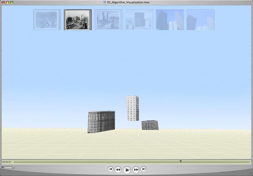
ering image appearance around unmeasured projections of
                                                                    3D points. In addition, with increasing numbers of misclas-
                                                                    sified points, structure segmentation decreases in quality, as
                                                                    fewer and fewer points have precisely the same dates of ex-
                                                                    istence. We hope to find more robust methods of segment-
                                                                    ing scene structure in order to automatically create high
                                                                    quality, time-varying 3D models from historical imagery.

                                                                    Acknowledgments
                                                                    This material is based upon work supported by the National Sci-
                                                                    ence Foundation under Grant No. IIS-0534330.

                                                                    References
                                                                     [1] J. F. Allen. Maintaining knowledge about temporal intervals.
                                                                         Commun. ACM, 26(11):832–843, 1983.
                                                                     [2] S. Badaloni, M. Falda, and M. Giacomin. Integrating quan-
                                                                         titative and qualitative fuzzy temporal constraints. AI Com-
                                                                         mun., 17(4):187–200, 2004.
                                                                     [3] R. Dechter, I. Meiri, and J. Pearl. Temporal constraint net-
                                                                         works. Artificial Intelligence, 49(3):61–95, May 1991.
                                                                     [4] D. Dubois, H. Fargier, and P. Fortemps. Fuzzy scheduling:
                                                                         Modelling flexible constraints vs. coping with incomplete
                                                                         knowledge. European Journal of Operational Research,
                                                                         147:231–252, 2003.
                                                                     [5] D. Dubois, H. Fargier, and H. Prade. Possibility theory in
                                                                         constraint satisfaction problems: Handling priority, prefer-
                                                                         ence and uncertainty. Applied Intelligence, 6:287–309, 1996.
                                                                     [6] O. D. Faugeras, E. Le Bras-Mehlman, and J. D. Boisson-
                                                                         nat. Representing stereo data with the Delaunay triangula-
                                                                         tion. Artif. Intell., 44(1-2):41–87, 1990.
                                                                     [7] M. Ge and M. D’Zmura. 4D structure from motion: a com-
                                                                         putational algorithm. In Computational Imaging., pages 13–
                                                                         23, June 2003.

Figure 10. Time-varying 3D model. Here, we see the scene as          [8] D. Jelinek and C. J. Taylor. View synthesis with occlu-
it appeared at 4 different times from the same viewpoint. This           sion reasoning using quasi-sparse feature correspondences.
result is generated automatically given 2D point correspondences         In Eur. Conf. on Computer Vision (ECCV), pages 463–478,
across 6 unordered images as input. We perform SFM, determine            2002.
occluding surfaces, compute the visibility matrix, solve the CSP     [9] D. D. Morris and T. Kanade. Image-consistent surface tri-
using local search to infer temporal ordering, group points based        angulation. In IEEE Conf. on Computer Vision and Pattern
on common dates of existence, compute 3D convex hulls, and tex-          Recognition (CVPR), volume 1, pages 332–338, 2000.
ture triangles based on where they project into each image.         [10] L. Sigal and M. J. Black. Measure locally, reason globally:
                                                                         Occlusion-sensitive articulated pose estimation. In IEEE
                                                                         Conf. on Computer Vision and Pattern Recognition (CVPR),
8. Conclusion                                                            pages 2041–2048, 2006.
   In this paper, we have shown that constraint satisfac-           [11] N. Snavely, S.M. Seitz, and R. Szeliski. Photo tourism: Ex-
tion problems provide a powerful framework in which to                   ploring photo collections in 3D. In SIGGRAPH, pages 835–
solve temporal ordering problems in computer vision, and                 846, 2006.
we have presented the first known method for solving this           [12] R. Sosic and J. Gu. 3,000,000 queens in less than one minute.
ordering problem. The largest obstacle to a fully automated              SIGART Bull., 2(2):22–24, 1991.
system remains the variety of misclassifications enumerated
                                                                    [13] C. J. Taylor. Surface reconstruction from feature based
above. In future work, we hope to extend the occlusion rea-
                                                                         stereo. In Intl. Conf. on Computer Vision (ICCV), page 184,
soning of our method to deal with occlusions by objects not
                                                                         2003.
explicitly modeled in the scene, such as trees, by consid-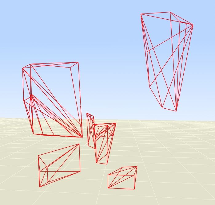
You can also read