Spacing and pressure to characterise arrival sequencing - Eurocontrol
←
→
Page content transcription
If your browser does not render page correctly, please read the page content below
Thirteenth USA/Europe Air Traffic Management Research and Development Seminar (ATM2019)

                        Spacing and pressure to characterise
                                arrival sequencing
                                         Raphaël Christien, Eric Hoffman and Karim Zeghal
                                                   EUROCONTROL Experimental Centre
                                                       Brétigny-sur-Orge, France

Abstract— This paper presents an analysis of the sequencing of
arrival flights at four European airports representative of                                    II.   STATE OF THE ART
different types of operation with more than 14000 aircraft pairs.            A comprehensive framework has been developed by the
The motivation is to better understand and characterise how               Performance Review Unit (PRU) of EUROCONTROL to
sequencing is performed in dense and complex environments                 characterise the performances of the arrival management
during peak periods. The analysis, purely data driven, focuses on
                                                                          process [3][4][5]. Two key elements introduced are the notions
the evolution of flight additional time, spacing deviation and
                                                                          of unimpeded time and additional time in the arrival sequencing
sequence pressure. The main results are: (1) at 15 minutes from
final, the average flight additional time varies from 4 to 6 minutes      and metering area, an area of 40NM (extended to 100NM in
(depending on the terrain), with a variability between ±2.5 and ±4        some analyses) from the airport. The unimpeded time is the
minutes; (2) at 15 minutes from final, the spacing deviation varies       transit time in the area in non-congested conditions. The
from ±3min to ±4min, and converges toward zero at 2min to final;          additional time is the difference between the actual transit time
(3) the sequence pressure (number of flights sharing the same             and the unimpeded time. It represents the extra time generated
arrival slot if no sequencing) is low at terminal area entry, and then    by the arrival management and “is a proxy for the level of
peaks at some distance/time from final before decreasing toward a         inefficiency (holding, sequencing) of the inbound traffic flow
target pressure of one flight per slot, closer to final. The pressure     during times when the airport is congested.” This indicator is
levels and their peak distribution over the terminal area differ          used (together with other indicators such as the flow
notably among destinations, highlighting the effect of the                management delay) in particular to compare the performance of
sequencing technique. Future work will involve analyzing high-            the main airports in Europe and in the U.S.A.[6].
pressure situations, in view of identifying the appropriate pressure
characteristics, i.e. trade-off between the required minimum                 The work presented here builds on these notions of
pressure and acceptable controller workload.                              unimpeded time and additional time in an area around the
                                                                          airport, and aims at characterising further, how the sequencing
   Keywords: arrival sequencing, aircraft spacing, approach               is performed. Similar types of indicators were also used at the
control, data analysis.                                                   level of individual flights, such as terminal area transition time
                                                                          deviation to detect any potential perturbations and assess the
                                                                          resilience of scheduled Performance-Based Navigation arrival
                       I.    INTRODUCTION
                                                                          operations [7].
   This paper presents an analysis of the sequencing of arrival
flights at four European airports representative of different types          When assessing the impact of new concepts in relation with
of operation (Dublin, Frankfurt Main, Madrid Barajas and Paris            sequencing, detailed analyses have been conducted [8][9][10].
Charles-de-Gaulle). The motivation is to better understand and            They consider different dimensions such as human factor (e.g.
characterise how sequencing is performed in dense and complex             workload, radio communications, instructions), flight efficiency
environments.                                                             (e.g. distance and time flown) and effectiveness (e.g. achieved
                                                                          spacing on final) using simulation data (human in the loop or
   The analysis relies on a data driven method introduced in              model based). To highlight the geographically based nature of
[1][2] that focuses on the dynamic of spacing over time,                  the sequencing activity, in particular late versus early
investigating in particular convergence and stability aspects.            sequencing actions, we introduced an analysis of instructions
This paper presents an extension towards the assessment of the            and eye fixations as a function of the distance from the final
sequence pressure, investigating the evolution of aircraft density        point [10].
in the sequence. The analysis considers peak periods during
which significant sequencing takes place, using nearly three                 All these studies aimed at assessing the impact of a new
months of data with in total more than 14000 aircraft pairs.              concept and considered the observable actions for sequencing.
                                                                          Although they informed on the sequencing activity of the
   The paper is organised as follows: after a review of related           controller, the dynamic of the spacing is not considered as an
studies, it will present the method and the indicators of                 element of the analysis. Furthermore, the need for operators
additional time, spacing deviation and sequence pressure. It will         related data, in particular instructions, makes uneasy the analysis
then go through the data collection and preparation. Finally, it          of current (live) operations. From a control theory perspective,
will present the analysis of results, followed by a discussion.           the spacing variable is the key element that should enable the

This study has been conducted as part of SESAR2020 programme (PJ01-02).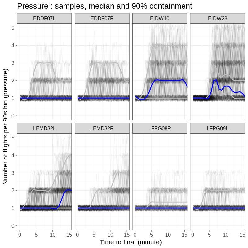
understanding of the human behavior. Here, we are not aiming           is illustrated on the left figure below: the thick blue trajectory is
at building a mathematical model of the approach controller,           considered the shortest one, except when crossing one of the
however as stated in [11], “control theory is a good foundation        orange trajectories which becomes for a short period the shortest
for developing the intuition and judgment needed for smart             one. The number of occurrences was nevertheless limited,
cognitive systems engineering”.                                        decreasing when getting close to final, and was mitigated by
                                                                       smoothing.
   A high level approach has been proposed in [12], relying on
three sets of indicators, in particular “flow based”, to build a          To overcome this limitation, we have refined the method by
global picture of the whole traffic situation in the terminal area,    considering segments/portions of trajectories. The minimum
however not informing on sequencing and spacing.                       time from a given point to a fix common point is now defined as
                                                                       the minimum time along all possible paths (from this point to the
   Numerous analysis of the spacing have been performed in the         fix common point), where a path is a succession of
context of airborne spacing when studying the performances of          segments/portions of trajectories connected to each other (see
different algorithms or of the flight crews [13][14][15][16][17].      figure right). Two portions of trajectories can be connected
Typical analyses involved in particular the relation between           provided a constraint of maximum bearing change to guarantee
spacing accuracy (control error) and number of speed                   a feasible turn. This constraint allows lifting the need to consider
changes/variations (control effort) as well as the impact of the
                                                                       trajectories of a same flow. Note that other constraints may also
resulting speed profile on the rest on the chain of aircraft           be considered (e.g. altitude or speed).
(reactionary effect). In all these cases, however, the situation
was such that the spacing could be defined as both aircraft               In practice, we define a graph with nodes matching the cells
followed known paths.                                                  and directed edges connecting the nodes together. We connect
                                                                       two nodes in the graph when a flight goes from one cell to the
   The issue being that, in the general case, the spacing variable     next in the traffic sample. The edge cost is the average duration
is not defined and formally does not exist. In vectoring for           to fly between the two nodes. We connect all the last nodes from
instance, while it is straightforward to measure the spacing at a      each trajectory to special sink node, corresponding to the final
final common point, it is unclear how to define the spacing            point. To get the minimum time from a given point to the final
between two aircraft being vectored on different paths but whose       point, we compute the minimum “distance” path (actually,
resume paths to the common point are unknown in advance. In            minimum duration path) from the corresponding node to the
this case, the spacing is part of the cognitive process of the         final point node in the graph, using the classical Dijkstra
approach controller and is not accessible.                             algorithm. This ensures that the minimum time from any point
                                                                       is a global minimum. Note that the nodes have a directional
                          III.   METHOD                                information (i.e. we can get 2 nodes at the same 2D location, one
   The method proposed, which extends the work presented in            used for North-bound traffic, and the other for West-bound
[1][2], is purely data driven and does not make any assumption         traffic) and that edges can only be created between nodes
in terms of sequencing techniques used or controller working           provided the constraint of maximum bearing change.
methods. It proposes three indicators for three different
perspectives: additional time for a single aircraft, spacing
deviation for a pair of aircraft, and pressure for a sequence of
aircraft. These indicators relies on a key element: the minimum
time.

A. Minimum time
   The minimum time corresponds to the notion of unimpeded
time introduced by the PRU [3][4][5] and defined as the transit
time in non-congested conditions in an area around the airport
(40NM or 100NM). This notion can be generalized to any point
in the area.                                                               Figure 1: Minimun time, initial version (left) and new version (right)

   Assuming a representative set of trajectories covering non-            This method better captures shortest paths and their
congested conditions, the minimum time from a given point to a         associated minimum times. However, the minimum times may
fix common point (e.g. final approach fix) was initially defined       rely on same common segments/portions of trajectories (e.g. in
as the flying time of the trajectory with the minimum flying time      final) and could be more sensitive to non-representative
among all the trajectories of the same flow passing through this       trajectories (too fast or too tight resulting from e.g. go-around or
point [1][2] (see following figure, left).                             calibration flight). This means that the outliers filtering stage
                                                                       becomes even more important.
  In practice, we discretise the area in the form of a map of cells,
each containing the minimum time from this cell to the final
approach fix.
   Although satisfactory, this method does not ensure a global
minimum at every point, thus could induce occurrences of
inaccurate values of additional time and spacing deviation. This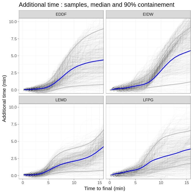
B. Additional time
   Similarly to the minimum time, the notion of additional time
of the PRU can also be generalized to any time for a given
trajectory. It can simply be defined as the difference between the
remaining flying time and the minimum flying time.
   The additional time represents the remaining delay to absorb:
starting from the total amount of delay at the entry of the area
and decreasing to zero at final point (a reversed definition could
be considered, starting from zero and ending at the total delay).
   In [2] we propose a decomposition of the additional time in
two parts: the “individual” part related to the spacing deviation                                Figure 2: Spacing deviation
of the considered pair, and the “queue” part related to the
“individual” part of all the preceding pairs in the sequence. The             With a spacing defined at all times, the sequencing can be
“queue” part will be propagated later to the considered pair and           formulated as a problem of manual control: the objective is to
will reflect the reactionary effect. Note: there may be also a third       set the spacing deviation to zero for all aircraft pairs in the
part for deviations related to other factors than arrival                  sequence. Considering the aircraft are set by default on their
sequencing (e.g. interaction with departures).                             shortest/fastest paths, the control action is to delay aircraft by
                                                                           acting on lateral (path stretching) and/or on longitudinal (speed
   We showed that the queue additional time constitutes the                reduction) dimensions. The additional time (delay) may thus
largest part of the additional time. This suggests that, while the         reflect the control effort applied on each aircraft.
pairwise spacing is established (and kept), there is some
sequencing effort even at a closer distance to the runway, due to             The intrinsic difficulty, beyond the handling of multiple pairs
the propagation of the individual additional time applied on the           in parallel, is the interdependency among these pairs with
preceding pairs. Although not considered here, this                        potential reactionary effect. Indeed, during peak periods, every
decomposition remains of interest and will be reflected in a               aircraft may be at the same time the trailer of a pair and the leader
different way by the sequence pressure introduced later.                   of the following pair. Hence, any action on an aircraft may
                                                                           impose to adjust the spacing on the rest of the sequence. This is
C. Spacing deviation                                                       typically the case when creating spacing to integrate two flows
                                                                           of aircraft. To limit this reactionary effect (and manage their
   The definition of spacing we propose relies on the                      workload), controllers tend to perform a progressive
combination of two existing notions: the minimum time                      convergence by adjusting the spacing more accurately as aircraft
introduced earlier and the constant time delay introduced by               get close to the runway, leaving a loose spacing when further
NASA for airborne spacing applications [13][14]. The constant              away and even creating some buffer (extra spacing) to anticipate
time delay was introduced to define a spacing deviation with               integration of aircraft.
aircraft following same trajectories; it is based on the past
positions of the leader aircraft with a given time delay
                                                                           D. Sequence pressure
corresponding to the required spacing. This notion can be
generalised to any aircraft trajectories.                                     As an attempt to get insight on the sequence, we propose an
                                                                           indicator that measures the aircraft density in the sequence and
   Let us consider a pair of consecutive landing aircraft denoted          will inform on the “pressure” at different time horizons. For this,
leader and trailer, with s their required time spacing1. Using the         we consider aircraft having a minimum time to go within the
constant time delay principle, the spacing deviation (or spacing           same time interval. Different lengths of time interval could have
error) at time t considers the current position of trailer at time t,      been considered, corresponding to different “granularity” of the
and the past position of leader at time t – s. Precisely, it is            measure. We have decided to consider a runway slot, set at 90
defined as the difference between the respective minimum times             seconds (wake turbulence categories not considered).
from these two positions (see figure below):
                                                                              We define the sequence pressure, for a flight, at a given time,
         spacing deviation (t) = min time (trailer (t)) –                  as the number of flights sharing the same minimum time to final
                                 min time (leader (t – s))                 ±45 seconds.
                                                                              Close to the final point, we expect a pressure of one aircraft
   This defines a spacing deviation at all times, with no                  (assuming a 90 seconds spacing on average), while it may vary
assumption regarding aircraft path/navigation: aircraft may be             at larger time horizons depending on the traffic demand and
following same or predefined trajectories, or may be on open               presentation (e.g. flights within a holding stack will generate a
vectors.                                                                   higher pressure).

1                                                                          required spacing was the final one. An analysis of the achieved spacing
  To simplify the interpretation of the spacing deviation curves, we
decided to set the final spacing deviation to zero, considering that the   at major European airports may be found in [18].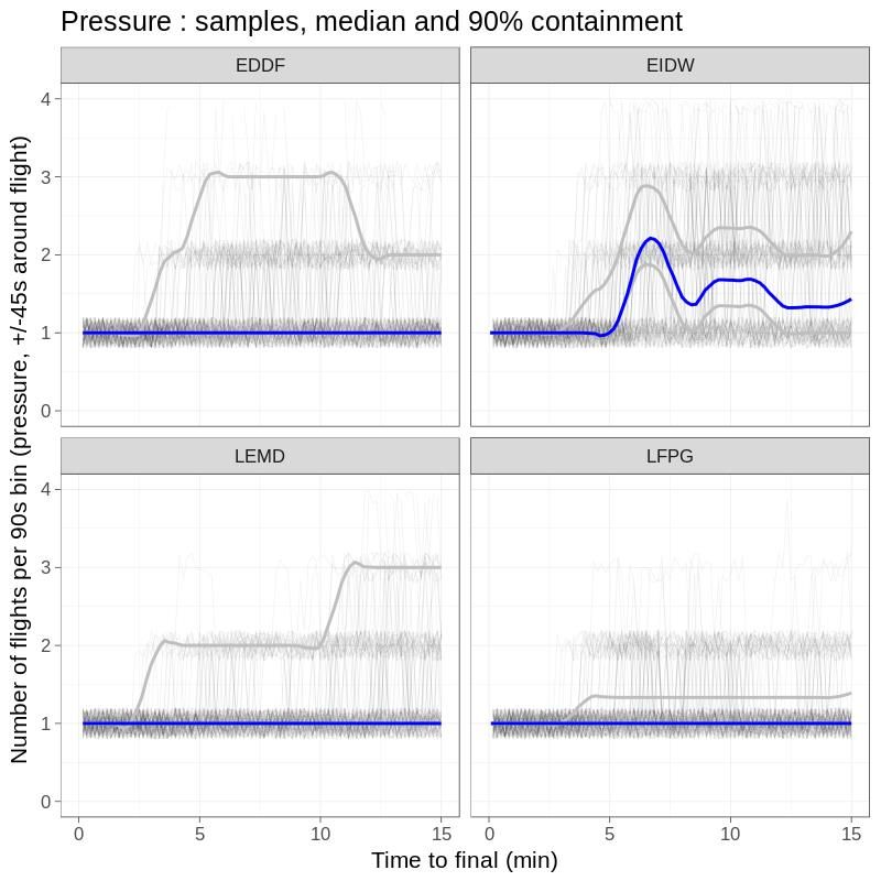
Figure 3: Sequence pressure

          IV.   DATA COLLECTION AND PREPARATION

A. Data collection
    We selected four airports representative of different types of
metering and sequencing: Dublin (EIDW) holding and point
merge [19], Frankfurt Main (EDDF) tromboning, Madrid
Barajas (LEMD) distant holding and vectoring, and Paris
                                                                                            Figure 4 : Tracks samples
Charles-de-Gaulle (LFPG) upstream metering and vectoring.
We consider a geographical focus area of 120NM radius around
each airport to fully encompass the metering and sequencing
area, with a minimum of 15 minutes flight time horizon.
    The dataset is based on 80 days selected at random from
2018 and consists of position reports with an average update rate
of 30 seconds (1 minute for LFPG) interpolated at a 10 seconds
rate by splines. Two filters have been applied to ensure
representativeness of data: (1) daytime operations (7h-21h local
time) to exclude night procedures; (2) ‘normal’ flights entering
and exiting the area, excluding go-arounds, flights with
exceptionally short or long flying time, or not flying over the
final approach fix. This makes the filtered sample sizes to be:
29713, 21505, 30141, and 27343 flights respectively for EDDF,
EIDW, LEMD and LFPG.
  The Figure 4shows a random sample of 1000 flights per airport
within the focus area, with all runway configurations
superimposed.

B. Data construction: minimum time
   As presented in section III, minimum times are computed in
all the cells of a 2D mesh covering the focus area based on all            Figure 5: Minimum time map toward one runway configuration
the recorded data. The cells differentiate themselves with
heading, but other factors may be considered to refine the
estimation like altitude, aircraft type, wind.                       C. Data selection: peak hours
   The selected cells size shall not be too large to allow for          We focus the analysis on peak periods during which
accurate trajectory deviations assessment. It shall not be too       significant sequencing is expected to take place. The
small, as future traffic position might not fall within existing     identification of the peak periods is based on the additional time
cells (surface coverage holes). For this case study, square cells    in the focus area (see next figure). We consider one hour periods
of 2/3NM width and 30 degrees heading bins were found to             with an average additional time per hour greater than the 75th
provide an appropriate trade-off.                                    percentile value per airport (periods may be consecutive). This
                                                                     corresponds to values from 5 to 8 minutes (upper part of the
   The Figure 5 shows cells of minimum times, for each airport,      boxes). Flights landing during these periods are considered for
toward one landing runway configuration. The colors represent        the analysis. At this stage of the data preparation, the dataset
the minimum time to final, from red (30 minutes) to blue (lower      consists of 7744, 5067, 8226 and 6645 flights, 317, 315, 224 and
than 1 minute).                                                      357 hours for EDDF, EIDW, LEMD and LFPG respectively.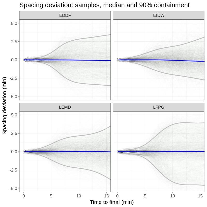
The level of additional time reflects the traffic demand and
                                                                      presentation in relation to the runway capacity. Typically, LFPG
                                                                      (lowest value) benefits from a metering performed upstream
                                                                      with the support of an arrival manager. In contrast, EIDW
                                                                      (highest value) receives traffic with limited look ahead and
                                                                      metering.
                                                                         At 5 minutes time to final, the median additional time for all
                                                                      destinations is usually lower than one minute, with little
                                                                      variability; this probably means that the sequence is stable but
                                                                      adjustments (path stretching or speed reduction) are still needed
                                                                      to maintain inter aircraft spacing.

          Figure 6: Average additional time per hour distribution

D. Data selection: aircraft pairs
   We further focus the analysis on aircraft pairs considered
close enough to require sequencing: we selected pairs with a
final spacing lower than 200 seconds at the final approach fix.
This makes the aircraft pairs sample sizes to be: 3307, 3104,
5295 and 2588 for EDDF, EIDW, LEMD and LFPG
respectively, making more than 14000 pairs. These sample sizes
are considered sufficiently large to be representative.

                        V.     DATA ANALYSIS
   The analysis relies on the three indicators introduced in
section III: additional time, spacing deviation and sequence
pressure. More precisely, it will investigate the evolution or
variations of these indicators at different time horizons, starting
at 15 minutes to final.
   The time horizon will be represented as “time to final”, i.e.                            Figure 7: Additional time
time to go along flown trajectory. It may have been represented
alternatively as “minimum time to final”, i.e. time to go as if
                                                                      B. Spacing deviation
flying fastest path. The “time to final” would correspond to an
aircraft view (flown trajectory) while the “min time to final” to        The following figure shows the spacing deviation (y-axis) vs.
a controller view (static map of minimum times).                      time to final (x-axis), for all landing runways per destination,
                                                                      with gray samples (1000 random cases per airport), 90%
   It is important to note that since the peak periods are based on   containment (lower curve corresponds to the 5th percentile and
different levels of congestion per airport, any comparison should     upper curve to the 95th percentile) and a median blue curve.
be made with caution.
                                                                         The median curves for all airports are aligned with the zero
A. Additional time                                                    deviation, result of the symmetry between the positive and
                                                                      negative spacing deviation values observed on the containment
   The following figure shows the additional time (y-axis) vs.        curves. One possible reason for that symmetry is that when the
time to final (x-axis), for all landing runways per destination,      spacing is increasing between two successive flights (i.e. the
with gray samples (1000 random cases per airport), 90%                trailer aircraft gets more additional time than its leader), this
containment (lower curve corresponds to the 5th percentile and        decreases the spacing with the flight after the considered trailer
upper curve to the 95th percentile) and a median blue curve.          aircraft (unless the third aircraft gets some additional time too to
  Focusing on the median curves, at 15 minutes to final, the          increase its spacing).
additional time is in the range 4-6 minutes (4 for LFPG, EDDF
and LEMD, 6 for EIDW). The range between the 5th and 95th
percentile at 15 minutes to final goes from 5 to 8 minutes (5 for
LFPG, 6 for LEMD, 8 for EDDF and EIDW).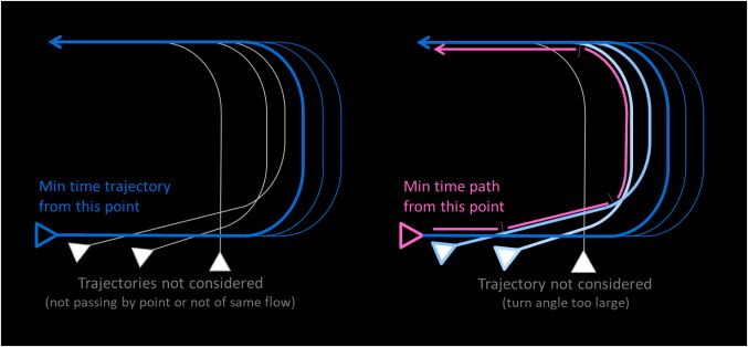
periods considered, before settling down. We may recall that
                                                                    EIDW has the highest additional time among the four airports.
                                                                       The upper containment curves converge to the target of one
                                                                    flight per slot (i.e. a pressure of 1), however they differ
                                                                    significantly among the airports. LFPG shows a constant low
                                                                    pressure, LEMD a high pressure at 15 minutes decreasing
                                                                    gradually, EDDF an increase at 5-10 minutes before settling
                                                                    down, and similarly for EIDW but settling down earlier at 5
                                                                    minutes.
                                                                       These observations may reflect the various types of metering
                                                                    and sequencing: metering upstream prior entry (and also
                                                                    probably runways not saturated) and sequencing close to final
                                                                    (vectoring) for LFPG; far metering (holding) followed by close
                                                                    sequencing (vectoring) for LEMD; metering (tromboning, sort
                                                                    of linear holding) followed by close sequencing (turn to final);
                                                                    and metering (holding) followed by sequencing achieved early
                                                                    (point merge, short linear holding at a fix iso distance from final)
                                                                    for EIDW.

                       Figure 8: Spacing deviation

   At 15 minutes from final, the 90% containment span ranges
from 6 (EIDW, ±3 minutes) to 7 minutes (EDDF and LEMD,
±3.5 minutes), while it is about 8 minutes (±4 minutes) for
LFPG. This deviation span at 10-15 minutes reflects the traffic
presentation (level of smoothing/bunching) and the ordering of
the aircraft (level of swap between flights).
   For LFPG, with a metering upstream, the high deviation span
may be due to an ordering different from the natural order. This
may result from the need to optimize the runway utilization (fill
any gaps between the two landing runways) and the landing
sequence (grouping by wake turbulence categories in a context
of significant traffic mix). In contrast, the deviation span is
reduced for EIDW probably due to a single landing runway and
less traffic mix.
  The spacing is obtained at 2 minutes to final for all
destinations (deviation span close to 0), however with different
convergence speeds. It is progressive for EIDW and LEMD,
while it is concentrated with a high speed in the 5-10min for
EDDF and LFPG.                                                                           Figure 9: Sequence pressure

C. Sequence pressure                                                   The figure below presents the same sequence pressure
   The following figure shows the sequence pressure (y-axis) vs.    information for the two most represented runways in our dataset
time to final (x-axis), for all landing runways per destination,    (graph top title made of ICAO destination and runway name),
with gray samples (1000 random cases per airport), 90%              by landing runway. We can see similar patterns for the different
containment (top curve 95th percentile, lower one, 5th percentile   runways, with the exception of a sustained period for EIDW10
flat equals to one except EIDW), and a blue curve representing      (long downwind) and a high pressure at entry for LEMD32L.
the average related to the 90% containment.
   The average curves remain constant at a pressure of one
flight, except for EIDW with values up to two flights between
10 and 5 minutes to final. This suggests some form of permanent
pressure during the peak periods, and higher in the area than at
entry. This may result from back propagation of the sequencing
(additional time), starting earlier and lasting longer than the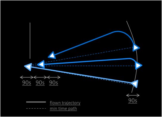
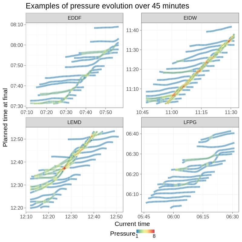
Figure 10: Sequence pressure (two most used runways per airport)              Figure 11: Example of seqeunece pressure over time

   The next figure presents one example of the pressure                     Finally, the next figure map shows the maps of average
evolution over time (per destination and toward a given runway)          pressure (one landing runway). This map corresponds naturally
selected among the highest-pressure cases. The x-axis is the             to the previous curves and confirms the location of the pressure
current time, the y-axis is the minimum time to final, and the           areas for each destination, reflecting the different types of
pressure is represented with a colour coding from blue (1 flight,        metering and sequencing.
i.e. the flight itself) to red (8 flights sharing the same ±45 slot)).
   For all destinations, near entry (left x-axis values), the
different pressure values shows different levels of bunching (e.g.
on these examples, some bunching patterns for EDDF and
LEMD). When getting closer to the final point (right x-axis
values), the time difference between consecutive flights in the
sequence is the required spacing (or more) and the pressure is
close to one (a must).
   Having a low pressure at entry does not guarantee it will stay
low, due to potential back propagation of additional time. For
EIDW and LEMD (holding), there is a “hot” spot, where the
flights are kept close to each other (in terms of arrival slot)
before being released at the right place in the landing sequence.
The pressure values do not evolve very much before entering
this spot. Note that for LEMD, since the holding stacks
(corresponding to the pressure red area) are at a relatively far
distance from final, there is still some pressure evolution (green
lines) occurring after it.
   For EDDF (tromboning), such a “hot” spot appears too, but
with smaller pressure values, while some pressure evolution is
visible before it, suggesting controller actions before the
tromboning area. For LFPG (upstream metering), the pressure
values never gets high, and we see slight pressure evolution at                          Figure 12: Pressure map toward one runway
different locations/time-to-go, suggesting a more scattered
management of the sequence.
VI.    DISCUSSION                             to multiple aircraft at this distance/time, hence to multiple
  This section is an initial attempt to interpret the results.        negative spacing deviations, which may be very demanding to
                                                                      set to zero, in particular with vectoring close to final. A high
   The arrival management relies on two objectives: (1)               pressure may result from and reinforce a back propagation of
maximise runway throughput and (2) minimise aircraft delay            additional time. Conversely, a low or moderate pressure at far
and controller workload. (1) requires to put a minimum pressure       distance corresponds to positive spacing deviations hence
on the runway (“reservoir” of aircraft) which may lead to aircraft    potentially under utilisation of the runway(s). Pressure is a way
delay and to a high workload close to final; (2) requires to          to meet the operational objective of maximising runway
manage the traffic presentation (smoothing/metering of traffic)       utilisation. It should be maintained at an appropriate range, not
which may lead to under utilisation of the runway(s) and              too far from final, when operating close to maximum runway
overloads in upstream sectors. A key aspect of sequencing             capacity. Moreover, when sequencing reshuffling is required,
during peak periods is the risk of knock-on effect, with back         having many aircraft sharing the same distance/time to final can
propagation of delays within the sequence.These considerations        be convenient for the controller, since he/she has only one time
raise the question of trade-off between pressure, delay and           reference to consider in building the sequence toward the final.
workload, which is specific to each environment.
                                                                         With this in mind and with caution, we may consider that the
   To better understand the sequencing work we have introduced        additional time of the four airports are quite high at 15 minutes
three indicators:                                                     to final (3 runway slots), but seems acceptable at 5 minutes
                                                                      (below 1 minute). The spacing deviation may also appear
  -    Additional time, focusing on one aircraft at a time,
                                                                      significant at 15 minutes (3 slots) but the gain due to possible
       representing the overall controller delay action. This is
                                                                      optimisation of the landing sequence would have to be assessed.
       the visible action of sequencing.
                                                                      The pressure shows varied situations, in particular when
  -    Spacing deviation, focusing on one aircraft pair at a time,    considering runways individually. It may be considered too low
       generating a part on trailer aircraft additional time. This    for LFPG08R if the runway is close to saturation, too high at
       is the cause for sequencing of this pair, but does not         entry for LEMD32L, too high during a long period for EIDW10;
       capture the whole sequence, and in particular any back         finally EDDF07L, EIDW28 and LFPG09L may appear as good
       propagation.                                                   candidates with a moderate pressure. The variations of the
                                                                      curves (and the number of outliers) for EIDW28 should
  -    Sequence pressure, focusing on the whole sequence,             nevertheless be investigated as may reflect some form of
       representing the density and how additional time may           sensitivity.
       back propagate.
                                                                         The various characteristics observed are directly related to
    The additional time represents the delay applied to an aircraft   operational objectives (runway throughput,..) and constraints
for sequencing and results from controller interventions (speed       (airspace, environment, ..), and also result from the way arrival
reduction or path stretching). In addition to degrading flight        management is operated, and in particular how working methods
efficiency (more track miles and less opportunities for               have been developed over years. The type of analysis presented
continuous descents), it may generate workload (controller and        may support adjustment or re-design of routes or operating
flight crew) depending on the technique used (open loop vs            methods, in order to better adhere the desired characteristics,
closed loop instructions) and proximity to final (critical phase of   specific to each environment.
flight). An increase of additional time may result from back
propagation of additional time downstream (see “queue
additional time” in section III 0). The additional time may thus                              VII. CONCLUSION
be considered as a form of necessary cost. It should be kept as          This paper presented an analysis of the sequencing of arrival
low as possible in particular near final, however a certain amount    flights at four European airports representative of different types
is inevitable during peak periods to keep pressure and flexibility.   of operation with more than 14000 aircraft pairs. The motivation
                                                                      is to better understand and characterize how sequencing is
   The spacing deviation represents the inter aircraft spacing
                                                                      performed in dense and complex environments during peak
error. Large deviations when entering the area may reflect
                                                                      periods. The analysis, purely data driven, focuses on the
bunches in the incoming traffic or a sequence order different
                                                                      evolution of flight additional time, spacing deviation and
from the natural order. Large negative deviations (i.e. not
                                                                      sequence pressure.
enough spacing) may result in significant delaying actions, but
may enable an optimisation of the landing sequence (runway               The main results are: (1) at 15 minutes from final, the average
balancing and re-arrangement depending on wake turbulence             flight additional time varies from 4 to 6 minutes (depending on
categories). Large positive deviations (i.e. too much spacing)        the terrain), with a variability between ±2.5 and ±4 minutes,
may result in gaps in the sequence. A variation of spacing            lower variability reflecting cases with sequence order nearly
deviation may results from back propagation of variations             frozen, higher variability, greater rescheduling; (2) at 15 minutes
downstream. Spacing deviation on final is thus an operational         from final, the spacing deviation varies from ±3min to ±4min,
objective. It should progressively converge to zero starting with     and converges toward zero at 2min to final; (3) the sequence
a spread at entry depending on the need to optimise the landing       pressure (number of flights sharing the same arrival slot if no
sequence.                                                             sequencing) is low at terminal area entry, and then peaks at some
                                                                      distance/time from final before decreasing toward a target
  The pressure represents the aircraft density in the sequence.
                                                                      pressure of one flight per slot, closer to final. The pressure levels
A high pressure at a given distance or time to final corresponds
and their peak distribution over the terminal area differ notably [17] D. Ivanescu, C. Shaw, E. Hoffman, K. Zeghal, “Towards Performance
among destinations, highlighting the effect of the sequencing Requirements for Airborne Spacing: a Sensitivity Analysis of Spacing
Accuracy”, 6th AIAA Aviation Technology, Integration and Operations
technique. Conference, Wichita, Kansas, USA, September 2006.
Future work will involve analyzing high-pressure situations, [18] G. Van Baren , C. Chalon-Morgan, V. Treve, “The current practice of
in view of identifying the appropriate pressure characteristics, separation delivery at major European airports”, 11th USA/Europe Air
Traffic Management R&D Seminar, Lisbon, Portugal, June 2015.
i.e. trade-off between the required minimum pressure and
[19] L. Boursier, B. Favennec, E. Hoffman, A. Trzmiel, F. Vergne, K. Zeghal,
acceptable controller workload. “Merging arrival flows without heading instructions”, 7th USA/Europe
Air Traffic Management R&D Seminar, Barcelona, Spain, July 2007.
REFERENCES
[1] R. Christien, E. Hoffman, A. Trzmiel, K. Zeghal, “Toward the
characterisation of sequencing arrivals”, 12th USA/Europe Air Traffic
Management R&D Seminar, Seattle, USA, June 2017.
[2] R. Christien, E. Hoffman, A. Trzmiel, K. Zeghal, “An extended analysis
of sequencing arrivals at three European airports”, AIAA Aviation
Technology, Integration, and Operations Conference, Atlanta, Georgia,
U.S.A., June 2018.
[3] EUROCONTROL, ATM Airport Performance (ATMAP) Framework,
Measuring Airport Airside and Nearby Airspace Performance, December
2009.
[4] EUROCONTROL, Performance Review Report, An Assessment of Air
Traffic Management in Europe during the Calendar Year 2017, May
2018.
[5] EUROCONTROL Performance Review Unit web site
http://ansperformance.eu
[6] EUROCONTROL and FAA, Comparison of Air Traffic Management-
Related Operational Performance: U.S./Europe 2017, March 2019.
[7] J. Jung, S. A. Verma, S. J. Zelinski, T. E. Kozon, L. Sturre, “Assessing
Resilience of Scheduled Performance-Based Navigation Arrival
Operations”, 11th USA/Europe Air Traffic Management R&D Seminar,
Lisbon, Portugal, June 2015.
[8] T. J. Callantine, P. U. Lee, J. Mercer, T. Prevôt, E. Palmer, “Air and
ground simulation of terminal-area FMS arrivals with airborne spacing
and merging”, 6th USA/Europe Air Traffic Management R&D Seminar,
Baltimore, Maryland, USA, June 2005.
[9] J. E. Robinson III, J. Thipphavong, W. C. Johnson, “Enabling
Performance-Based Navigation Arrivals: Development and Simulation
Testing of the Terminal Sequencing and Spacing System”, 11th
USA/Europe Air Traffic Management R&D Seminar, Lisbon, Portugal,
June 2015.
[10] I. Grimaud, E. Hoffman, L. Rognin, K. Zeghal, “Spacing instructions in
approach: Benefits and limits from an air traffic controller perspective”,
6th USA/Europe Air Traffic Management R&D Seminar, Baltimore,
Maryland, USA, June 2005.
[11] M. Mulder, M. M. Van Paassen, J. M. Flach, R. J. Jagacinski,
“Fundamentals of Manual Control Theory,” in The Occupational
Ergonomics Handbook (Second Edition) – Fundamentals and Assessment
Tools for Occupational Ergonomics, W. S. Marras and W. Karwowski,
Eds. CRC Press, Taylor & Francis, London, 2005, pp. 12.1–12.26, ISBN
0849319374.
[12] L. Yang, S. Yin, M. Hu, Y. Xu, “A case study of non-linear dynamics of
“human-flow” behavior in terminal airspace”, 12th USA/Europe Air
Traffic Management R&D Seminar, Seattle, USA, June 2017.
[13] J.A. Sorensen, T. Goka, “Analysis of in-trail following dynamics of
CDTI-equipped aircraft”, Journal of Guidance, Control and Dynamics,
vol. 6, pp 162-169, 1983.
[14] J.R. Kelly, T.S. Abbott, “In-trail spacing dynamics of multiple CDTI-
equipped aircraft queues”, NASA, TM-85699, 1984.
[15] K. Krishnamurthy, B. Barmore, F. Bussink, “Airborne precision spacing
in merging terminal arrival routes: a fast-time simulation study”, 6th
USA/Europe Air Traffic Management R&D Seminar, Baltimore,
Maryland, USA, June 2005.
[16] E. Alonso, G.L. Slater, “Control Design and Implementation for the Self-
Separation of In-Trail Aircraft”, AIAA Aviation, Technology,
Integration, and Operations Conference, Arlington, Virginia, USA,
September 2005.You can also read