East Antarctica magnetically linked to its ancient neighbours in Gondwana
←
→
Page content transcription
If your browser does not render page correctly, please read the page content below
www.nature.com/scientificreports
OPEN East Antarctica magnetically
linked to its ancient neighbours
in Gondwana
Jörg Ebbing1*, Yixiati Dilixiati1, Peter Haas1, Fausto Ferraccioli2,3 &
Stephanie Scheiber‑Enslin4
We present a new magnetic compilation for Central Gondwana conformed to a recent satellite
magnetic model (LCS-1) with the help of an equivalent layer approach, resulting in consistent
levels, corrections that have not previously been applied. Additionally, we use the satellite data
to its full spectral content, which helps to include India, where high resolution aeromagnetic data
are not publically available. As India is located north of the magnetic equator, we also performed
a variable reduction to the pole to the satellite data by applying an equivalent source method. The
conformed aeromagnetic and satellite data are superimposed on a recent deformable Gondwana plate
reconstruction that links the Kaapvaal Craton in Southern Africa with the Grunehogna Craton in East
Antarctica in a tight fit. Aeromagnetic anomalies unveil, however, wider orogenic belts that preserve
remnants of accreted Meso- to Neoproterozoic crust in interior East Antarctica, compared to adjacent
sectors of Southern Africa and India. Satellite and aeromagnetic anomaly datasets help to portray the
extent and architecture of older Precambrian cratons, re-enforcing their linkages in East Antarctica,
Australia, India and Africa.
Defining the architecture of the lithosphere under the thick ice cover of Antarctica is of wide interest as large parts
are still blanks on geological maps (Fig. 1 and recent Gondwana m ap1). Novel methods and data are needed to
enhance our current knowledge and link the geology from the few outcrops at the coast to that under the i ce2,3.
For example, in a recent study, heat-flow values from the formerly adjacent neighbours were interpolated into
East Antarctica, deriving a map significantly different from previous interpretations4. A second study uses a set
of geophysical data and models to define lithospheric domains in East Antarctica by statistical analysis3. Both
these statistical methods in their simplicity provide new insights, but have limitations, mostly due to the sparse
coverage of data used.
Magnetic data collected over the last 50 years, although with varying resolution and accuracy, covers Ant-
arctica and its ancient continental neighbours. Previous studies have shown that magnetic data, especially when
interpreted jointly with geochronological, geochemical, geophysical and palaeomagnetic datasets, helps identi-
fying fundamental links between formerly adjacent neighbours within the Gondwana, Rodinia and Columbia
supercontinents5,6. These links are highly relevant for global supercontinent studies as current plate reconstruc-
tions still vary considerably, both in terms of defining the relative positions and the tectonic processes that
affected different continents.
In this context, Antarctica has a special role as it holds a key position in a Gondwana framework7–9 but its
geology is mostly hidden under its thick ice cover. Therefore, reconstructing the position of Antarctica helps to
extrapolate the geology from the former adjacent neighbours. For example, such reconstructions were used to
discuss the structural setting of East Antarctica with respect to the setting of Southern Australia and showed
that the magnetic data indicate the continuation of the Australian geology under the ice of Antarctica10–12. That
link between Antarctica and Australia has been studied in detail using aeromagnetic data of comparable quality.
Studies on the link between Antarctica and Southern Africa, however, have often had a focus on Dronning Maud
Land on the Antarctic side or relied on low-quality global magnetic compilations outside Antarctica13–15. Similar
observations can be made for the link between India and Antarctica, which has been studied albeit without using
magnetic data16. A reason for this is that aeromagnetic data for the Indian subcontinent are not openly available
and in state-of-the-art global compilations models like E MAG2v317 are indicated to be of low quality.
Resolution and accuracy are in general an issue when using global magnetic anomaly compilations to derive
tectonic interpretations and supercontinent linkages. For example, EMAG2v3 has a nominal resolution of 2
1
Institute for Geosciences, Kiel University, Kiel, Germany. 2OGS, Trieste, Italy. 3British Antarctic Survey, Cambridge,
UK. 4Witwatersrand University, Johannesburg, South Africa. *email: Joerg.Ebbing@ifg.uni-kiel.de
Scientific Reports | (2021) 11:5513 | https://doi.org/10.1038/s41598-021-84834-1 1
Vol.:(0123456789)
www.nature.com/scientificreports/
Figure 1. (A) Conformed aeromagnetic data, (B) Satellite model LCS-1 after variable reduction to the pole,
orld28.
represented at 5 km ellipsoidal height. (C) Surface geology as represented in the Geological Map of the W
The geological units are: 1: Cenozoic, 2: Mesozoic, 3: Upper Paleozoic, 4: Lower Paleozoic, 5: Neoproterozoic,
6: Mesoproterozoic, 7: Paleoproterozoic, 8: Archean, 9: Large Igneous Provinces, 10: Glaciers and Ice. For more
details, see28. All data sets are rotated back to 200 Ma with the deformable plate m
odel5.
arc-minutes, but data content is highly heterogeneous over the globe. That relates to accuracy and resolution,
but also the treatment of the long-wavelength content that is notoriously unreliable. The maximum wavelength
contained in any dataset is limited by the survey extent and often one refers to a spectral gap between satellite
and aeromagnetic data. To address this spectral gap, in Australia a number of long-haul flight lines had been
acquired18–20. Still, the long-wavelength range in the most recent release has been replaced by satellite data due
to their increased accuracy. A number of studies have made use of recent releases of the satellite lithospheric
magnetic field to replace the long-wavelength part of aeromagnetic surveys with satellite d ata21,22. For example,
in the Circum-Arctic region, the long-wavelength aeromagnetic data were replaced with satellite data using a
cut-off filter of 400 and 330 k m22. This cut-off relates to the maximum spatial resolution of the early generation
of satellite m odels23–25 and corresponds to the maximum reliable wavelength of typical aeromagnetic surveys.
The resolution of satellite-derived magnetic field models is limited by the orbit height, instrumentation and
mission period. Since 2013, the Swarm satellite mission from the European Space Agency has been continuously
measuring the Earth’s magnetic field. The mission consists of three-satellites at different altitudes and with chang-
ing orbit i nclinations25,26. The addition of these data to the data from previous satellite missions (e.g. CHAMP,
Oersted) helps to increase spectral accuracy and appears in the Swarm-derived lithospheric field model LCS-1
providing reliable wavelengths in some regions to 250 k m25. However, in Polar Regions, the noise in satellite data
is greater than at mid-latitudes27. Due to the increased noise, the lithospheric field estimates are less accurate for
wavelengths larger than 300 km wavelength.
Here, we conformed the available aeromagnetic compilations for Antarctic and its neighbouring continents
Australia and Southern Africa to satellite data. This process results in a homogeneous data representation across
Scientific Reports | (2021) 11:5513 | https://doi.org/10.1038/s41598-021-84834-1 2
Vol:.(1234567890)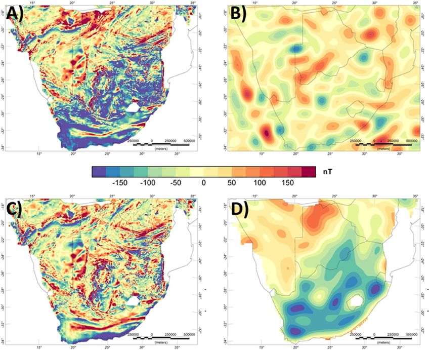
www.nature.com/scientificreports/
Figure 2. Lithospheric magnetic anomaly of Southern Africa. (A) Original aeromagnetic c ompilation29, (B)
Satellite-derived model LCS-1, (C) Conformed aeromagnetic and satellite model. (D) Difference of (A,C).
the heart of Gondwana. We discuss the value of the conformed data and the satellite data itself by linking up
anomalies between Southern Africa, Australia and East Antarctica. In addition, we look at the satellite data link
to India to its Antarctic counterpart.
Conforming satellite magnetic and aeromagnetic data
To illustrate the different steps in homogenising the aeromagnetic data, we choose the area of Southern Africa
(Fig. 2). Two aeromagnetic grids cover the area of South Africa, one made publicly available in 2 000s29 and the
second, an updated version, released in 201930. In the original compilation a difference in the main level of >
-100 nT can be observed between South Africa and its northern African neighbours (Fig. 2A), while in the latest
release South Africa is shifted by ~+50 nT (not shown here).
The difference in the level could be misinterpreted as reflecting fundamental variability in crustal-scale geol-
ogy or thermal state. E.g. the long to mid wavelength field is often used to estimate the Curie i sotherm31, but can
also relate to differences in crustal architecture32, upper mantle magnetisation33 or a combination of thermal and
structural properties34. For this area, the pattern partially correlates with some of the main tectonic features of
the area such as the boundaries of the Kaapvaal Craton to its surrounding. An indication, that this feature here
is instead an artefact of processing comes from the fact that the shift values for the two generations of compila-
tion have an opposite sign.
Therefore, we replace the long-wavelength part of the original 2000s Southern Africa aeromagnetic compi-
lations with the satellite model LCS-1 (Fig. 2B). For this, we use an equivalent layer approach and replace the
data up to spherical harmonic degree 130 (corresponding to ~300 km wavelength) with satellite data (see Data
and Methods for more details). The resulting conformed grid is spectrally consistent and still contains the high-
frequency information of the original compilation.
The long-wavelength part of the aeromagnetic compilation, if accurately estimated, is expected to be similar
to satellite derived data. However, the long-wavelength part shows differences of more than -100 nT for South
Africa and considerably less differences for the countries to its north as can be seen in the correction applied to
the data (Fig. 2D).
As mentioned, for South Africa, an updated aeromagnetic grid is as well available30, having an apparent
higher resolution, due to the inclusion of more recent surveys, and with an opposite sign shift of 50 nT for the
Scientific Reports | (2021) 11:5513 | https://doi.org/10.1038/s41598-021-84834-1 3
Vol.:(0123456789)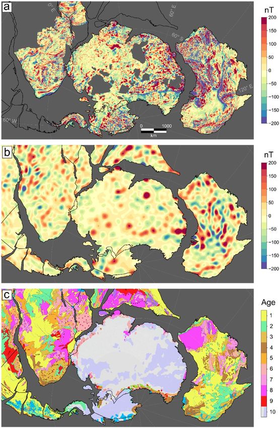
www.nature.com/scientificreports/
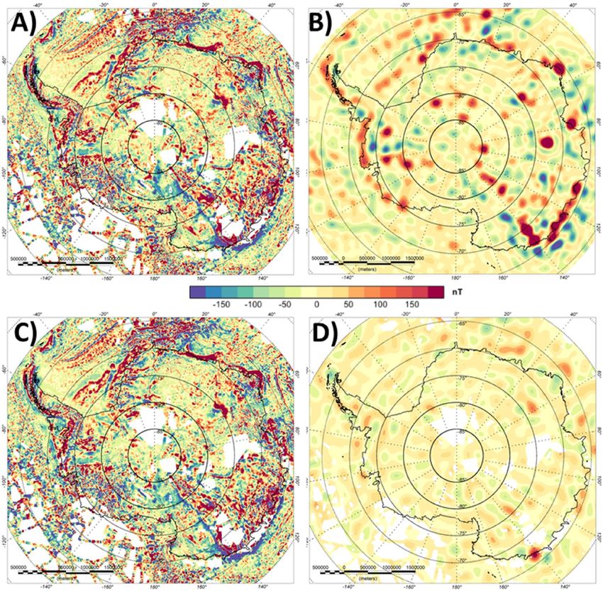
Figure 3. Lithospheric magnetic anomaly for Antarctica. (A) Original ADMAP-2 compilation35. (B) After
conforming ADMAP-2 to the satellite model LCS-1. (C) EMAG2v317.
long-wavelength in South Africa. Conforming this grid to the satellite model results again in a long-wavelength
trend correction and in a homogenous anomaly map that still reflects the major crustal domains of Southern
Africa.
We applied the same procedure to the Australian and Antarctic datasets (see Data and Methods). For Aus-
tralia, the differences in the long-wavelength range are relatively small. The differences result from the use of a
different satellite model as compared to original Australian compilation, where the long-wavelength part was
replaced by the satellite model MF-724. Here, we replace instead the long-wavelength components with the
more recent LCS-1 model for improved consistency between the compilations for the individual continents we
examined.
More interesting are the differences for Antarctica. For the ADMAP-2 compilation all surveys have been
corrected for the same geomagnetic reference model, but no correction for satellite data has been applied35.
Nevertheless, the long-wavelength component of ADMAP-2 still corresponds very well with the satellite-derived
model. Conforming the Antarctic aeromagnetic compilation to the satellite model leads to sharpening of some
anomalies with the main differences between satellite and aeromagnetic data in the long-wavelength range being
correlated to the line density and general data coverage (Fig. 3). In areas where the aeromagnetic data coverage
is denser, the location of the anomalies are similar, but shapes and extents may vary.
Unfortunately, not all of the continents surrounding Antarctica, have aeromagnetic compilations in the public
domain, e.g. India. Therefore, one might consider using data from global compilations to fill the gaps. In Fig. 3,
we compare the conformed satellite-aeromagnetic anomaly map to the global model EMAG2v3 for Antarctica.
The comparison shows that most of the details seen in our satellite-corrected aeromagnetic data compilation
are less clear in the global compilation. EMAG2v3 comes with a data quality measurement that shows the data-
set does not contain consistent high-quality measurements for this area. It is evident that EMAG2v3 is only a
smoothed representation of the aeromagnetic datasets and some of the linear features appear blurred and do
not show the strike directions.
For India, the quality of the data in EMAG2v3 is even w orse17 and hence any correlation of the features to
East Antarctica is even more complicated. Another issue is the direction of the inducing main field. Induced
magnetisation is commonly assumed to be the dominant magnetisation over the continents, while remanent
magnetisation dominates over the oceanic plates36. The direction and strength of the magnetic main field changes
from the poles to the equator. While the strength of the field governs the amplitudes of the anomalies, the incli-
nation of the field governs the shape and location of the anomalies. For a vertical field, the peak anomalies are
located over the source body and side slopes are small. For an inclined field, a typical magnetic dipole anomaly
is observed, where none of the anomalies are necessarily located directly over the source. For Polar Regions,
such as Antarctica, this directional effect is often ignored, but for inclinations less than 70 degrees, the changes
become more important.
While the inclination does not represent the inclination during break-up, it implies that simple reconstruc-
tions show rock formations adjacent to each other that actually have a completely different orientation in the
Earth magnetic field because their magnetic field is based on the present day continent layout. The inclination
in Southern Africa and Australia is around 50 degrees and increases to 90 degrees in Antarctica. India is located
slightly north of the magnetic equator (where inclination is zero). Therefore, after conforming the compilations
to a common satellite model, we performed a reduction to the pole considering the variable direction of the
magnetic field (Fig. 5 and see Methods section). However, this correction should consider the orientation of the
magnetic field during the time of acquisition. Such information is next to impossible to retrieve for all the surveys
acquired over more than 60 years. We applied the correction only to the satellite model for which a reduction
to the pole (RTP) with a common datum is straight forward. Common spectral methods for reduction to the
pole fail for satellite data. Instead, we calculated a RTP satellite model with an equivalent source method. This
method also does not suffer from the numerical instability at the magnetic equator as Fourier-based methods
do, but as it is computationally expensive was not used for the aeromagnetic data sets.
Scientific Reports | (2021) 11:5513 | https://doi.org/10.1038/s41598-021-84834-1 4
Vol:.(1234567890)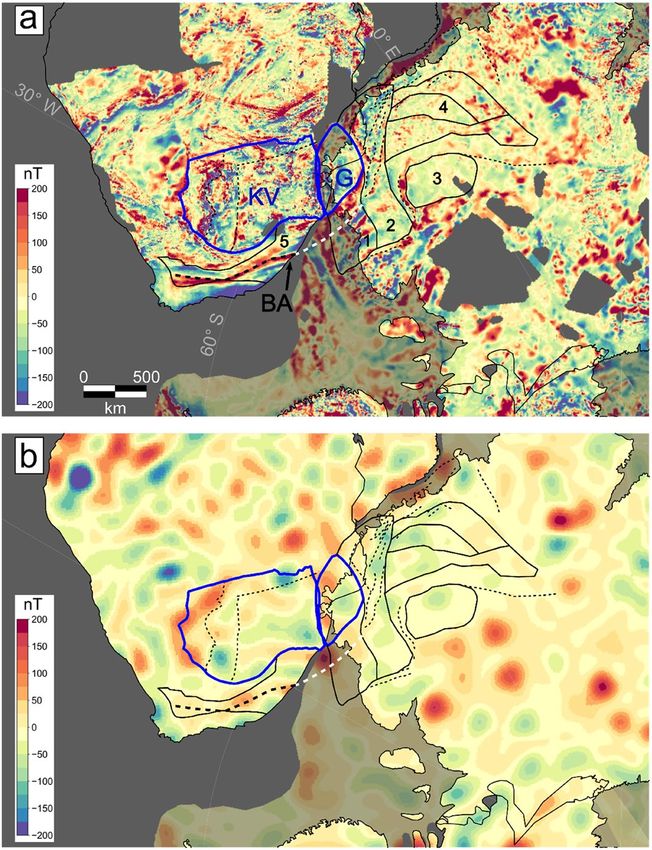
www.nature.com/scientificreports/
Figure 4. Zoom in on the South Africa-Antarctica connection. (a) Combined aeromagnetic-satellite model.
The connecting cratons are marked as blue contours. KV: Kaapvaal, G: Grunehogna Craton. Beattie Magnetic
Anomaly (BA) is indicated as thick dashed line. Solid black contours represent selected tectonic units of
Antarctica older than 200 Ma. 1: Natal type terrane boundaries. 2: Maud Belt, 3: Valkyrie Craton, 4: Tonian
Antarctic Super Terrane (TOAST). Contour 5: Natal terrane. Dashed lines indicate several fracture zones in
South Africa and Dronning Maud Land, White dashed line: Continuation of the Beattie Magnetic Anomaly, (b)
Satellite data LCS-1. Both data sets have been reduced to the pole and are represented at 5 km height. All data
sets are rotated back to 200 Ma. Semi-transparent anomalies indicate aeromagnetic anomalies on the continental
margin.
Discussion
Two things are of interest in interpreting the conformed aeromagnetic and satellite data: (1) the internal structure
of the continents, especially East Antarctica, and (2) the link to its adjacent parts in a Gondwana framework.
Figures 1, 4 and 5 show the results in a pre-Gondwana break-up configuration ca 200 Ma ago based on a deform-
ing plate model5.
The area, where the integration of satellite and aeromagnetic data has changed the most is Southern Africa.
Figure 4 shows a zoom to the link between South Africa and East Antarctica. It has been already discussed that
the Beattie anomaly can be linked to an anomaly with similar amplitude and trend in Dronning Maud Land,
Antarctica37 that sharply terminates along the western orogenic front of the East African O rogen38–40. Recently,
it was suggested by geological-petrological modelling that the Beattie anomaly is linked to a shear zone near the
southern boundary of the Natal t errane41. The anomaly is part of a family of anomalies, one of which correlates
with outcropping shear zones in the Mesoproterozoic Natal belt for which a complex remanent magnetisation
was suggested43. However, the corresponding Antarctic anomalies have a higher amplitude (Fig. 4), due to the
fact that the corresponding sources on the South African side are covered by sediments of the Karoo basin. In the
satellite data, a weak imprint of the Beattie anomaly is visible, which confirms its regional significance (Fig. 4).
The satellite data show their potential in illuminating the link between India and East Antarctica (Fig. 5). In
the original satellite data, the Indian-Antarctic link is not very pronounced, but after the RTP correction, the
anomalies line up, indicating a continuation of the Indian geological provinces under the Antarctic ice. Satellite
data are limited in their ability to resolve local structures, but are expected to reflect the major tectonic setting.
The match-up of the India and Antarctic pieces suggest that the sources are upper crustal Precambrian basement
that has not been significantly altered by continental break-up.
Scientific Reports | (2021) 11:5513 | https://doi.org/10.1038/s41598-021-84834-1 5
Vol.:(0123456789)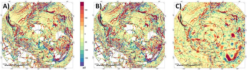
www.nature.com/scientificreports/
Figure 5. Zoom in on the India-Antarctica connection. (a) Original satellite mode LCS-1, (b) RTP corrected
satellite model. Both data sets are represented at 5 km height. All data sets are rotated back to 200 Ma. Semi-
transparent anomalies indicate aeromagnetic anomalies on the continental margin.
However, future more detailed analysis should consider the importance of remanent magnetisation, as many
of these rock formations are billions of years old and gained parts of their magnetic orientation during emplace-
ment or formation when the Earth’s magnetic field had a different orientation. Ideally, to increase the correlation
of the Indian continent to Antarctica, one would need to process the aeromagnetic data for India in the same
manner as for the other continents, if the survey data became available.
Conclusions
Aeromagnetic data are important when discussing the tectonic setting of the continents, especially in a plate
reconstruction. However, aeromagnetic compilations should be conformed to satellite data to be spectrally con-
sistent, especially when these compilations are based on multiple surveys acquired over a long time period. The
increased resolution and accuracy of satellite data allows confident identification of the main tectonic signatures
in the data sets. In this study, the higher resolution of the conformed compilations further aids the interpretation
of the links between East Antarctica and its former Gondwana neighbours. That is clearly seen both in the well-
established link between Australia and Antarctica and the less-explored link between the interior of Southern
Africa and Antarctica. RTP satellite data show furthermore the huge potential for reinterpreting the link between
India and East Antarctica, when aeromagnetic data over the Indian subcontinent become available.
Less important here is the exact geometry of the margins and break-up, but that properties from the interior
of the continents can be linked to their previous neighbours. Here, we emphasis this for East Antarctica. A
natural next step would be to apply multivariate analysis3 adding the magnetic data. That would allow definition
of lithospheric domains for East Antarctica in line with the tectonic setting of Australia, Southern Africa and
possibly India. This furthermore could help to interpolate other sparse measurements into East Antarctica or
to define statistical correlations which can be used for predictions. A current application is deriving geothermal
parameters under the Antarctic ice45. Guided interpolation of geothermal heat-flow values using the magnetic
field is possible, as well as cluster analysis and machine learning approaches, where statistically correlation are
exploited for improved predictions.
Scientific Reports | (2021) 11:5513 | https://doi.org/10.1038/s41598-021-84834-1 6
Vol:.(1234567890)
www.nature.com/scientificreports/
Figure 6. Lithospheric magnetic anomaly of Australia. (A) Original aeromagnetic c ompilation20, (B) Satellite-
derived model LCS-1, (C) Conformed aeromagnetic and satellite model, (D) Difference between (A,C).
Data and methods
Australia, Southern Africa and Antarctica are three of the areas of the world with particularly comprehensive
aeromagnetic data coverage (see Figures 2, 6 and 7). In Australia and Southern Africa, widespread high-reso-
lution aeromagnetic data acquisition has primarily been motivated by mineral resource m apping19,29, while in
Antarctica the focus has mostly been on systematically exploring subglacial geology and defining large-scale
crustal architecture13,35,44. Therefore, the survey parameters (e.g. survey height and line spacing) typically adopted
in the three continents are quite different.
Over Australia more than 800 individual surveys are nowadays included in Geoscience Australia’s National
Airborne Geophysical Database (NAGD) that contains more than 31 million line kilometres of total field mag-
netic intensity data. Since 1990, surveys have usually been conducted with flight line spacing of 400 metres or
less19. To reduce long-wavelengths errors, high-altitude airborne traverse data were used, which significantly
improved the intermediate wavelengths from 100 to 500 km. For edition 5 of the magnetic anomaly map for
Australia, which is used here, the long-wavelength part (>1000km) has been replaced with the satellite magnetic
model MF-6.
Systematic data acquisition in Antarctica started as early as the International Geophysical Year 1957–1958. A
wealth of modern airborne geophysical surveys, including airborne gravimetry and aeromagnetic data acquisi-
tion over previously largely unexplored Antarctic frontiers, such as the Gamburtsev Subglacial Mountains46 and
Wilkes Land in East Antarctica11 was stimulated by the International Polar Year 2007/2008. The first Antarctic
magnetic anomaly compilation (ADMAP‐1) was produced in 2001 from more than 1.5 million line kilometres of
shipborne and airborne m easurements47. This was succeeded in 2018 by the second-generation Antarctic mag-
netic anomaly compilation (ADMAP-2) that includes more than 3.5 million line‐km of aeromagnetic and marine
magnetic data that more than doubles the initial near‐surface database35. Large-scale international aeromagnetic
Scientific Reports | (2021) 11:5513 | https://doi.org/10.1038/s41598-021-84834-1 7
Vol.:(0123456789)www.nature.com/scientificreports/
Figure 7. Lithospheric magnetic anomaly of Antarctica. (A) Original aeromagnetic c ompilation35, (B) Satellite-
derived model LCS-1, (C) Conformed aeromagnetic and satellite model, (D) Difference between (A,C).
exploration in Antarctica has continued since ADMAP-2, with major more recent surveys flown e.g. over the
Recovery and South Pole f rontiers48,49.
For Southern Africa (Fig. 2), two modern compilations exist from the Council for Geoscience, Republic of
South Africa, who began collecting and compiling aeromagnetic data in the 1970s. Similar programs of collect-
ing aeromagnetic data throughout the Southern Africa region have resulted in nearly complete aeromagnetic
coverage of South Africa, Namibia, Botswana and Zimbabwe. The Council for Geoscience has compiled all of
these magnetic data available in southern Africa and has gridded the data at one km grid spacing 29. Because
the data have a relatively large line spacing (1 km), they were initially only used for large scale mapping, mainly
for mapping the Kaapvaal Craton boundary, lithology identification and for defining important linear magnetic
features50. An update for the Republic of South Africa is now available30. The long-wavelength part between the
two compilations is quite different, while the short-wavelength part is very similar, again confirming the use of a
common reference model. Quantitative interpretations of the higher resolution data concentrated on individual
targets such as the Beattie magnetic a nomaly41,51,52.
The satellite model for the lithospheric magnetic field is LCS-125. LCS-1 contains the spherical harmonics
from degree and order 15-185. The lower order spherical harmonics are associated with the main (core) field and
omitted from the lithospheric field part. In comparison to previous models, LCS-1 represents the field to a high
spherical harmonic degree by providing coefficients to 185 corresponding to ~220 km wavelength. Based on the
data from pre-Swarm satellite mission data only, earlier models limited the representation to degree 70 (~600
km), 85 (550 km) or 130 (300 km). For LCS-1, the spectral range to degree 130 is globally consistently estimated,
while for the higher spherical harmonics, especially in Polar Regions, the noise increases, making the representa-
armonics25.
tion less accurate. Still, for Australia there is lithospheric signal contained in the higher spherical h
Scientific Reports | (2021) 11:5513 | https://doi.org/10.1038/s41598-021-84834-1 8
Vol:.(1234567890)www.nature.com/scientificreports/
Conforming aeromagnetic compilation to satellite model
To homogenize the data, we applied an equivalent dipole layer approach coupled with spherical harmonic
representation54. The reason for using an equivalent source method is, that the Fourier based methods result
in artefacts when applied to global long-wavelength satellite data and suffer from instabilities at the magnetic
equator. Equivalent sources do not suffer from this instability, but require extensive computational resources.
Hence for the aeromagnetic surveys a simplification has to be made.
1) For estimating the magnetic parameters of the equivalent dipole layer, we used BiCGSTAB iterative inversion
method. For the satellite data, we located the equivalent dipole layer at 30 km beneath the reference level with
a horizontal spacing of 25 km corresponding to the data spacing. These values were found to best represent
both the spectral content at an observation height of 400 km and near surface. The field was inverted using
the direction of the main field model CHAOS-653 at each dipole location. No amplitude correction was
applied. CHAOS-6 was also used as reference model for LCS-1.
2) From the equivalent dipole layer, we forward calculate the RTP model at 5 km ellipsoidal height for a vertical
field and a constant field strength.
3) For the aeromagnetic data, we also applied an equivalent dipole layer representation, but for computational
reasons, first performed a simple resampling of the data data to ~22 km (0.2 degree equiangular) resolution
for Australia and Southern Africa and ~44 km (equidistant) for Antarctica. This step did not affect the long-
wavelength content of the data, but obviously limited the short-wavelength content. The equivalent sources
were again located at 30 km beneath the reference level and were calculated using CHAOS-6 as main field.
4) Next, we estimated the spherical harmonic coefficients from the equivalent layer for both the satellite and
aeromagnetic data by calculating the coefficient for each dipole and summing up their individual effects.
Spherical harmonic coefficients have been calculated to degree and order 180 for satellite data and 720 for
the aeromagnetic data sets
5) For spherical harmonic coefficients up to degree and order 130, the difference between the satellite and
aeromagnetic data has been calculated and used to correct the original aeromagnetic data.
Plate‑tectonic illustrations
Figures 1, 4 5 and the movie in the supplementary material have been made with GPlates (http://www.gplat
es.org/) using its global reconstruction files. The supplementary animation provides an example for the last 200
My of plate tectonics centred over Antarctica. The movie illustrates with the conformed aeromagnetic data and
satellite data as infill, where no aeromagnetic data are available, the link between Antarctica and the adjacent
continents. The plate-tectonics illustration was done in GPlates (https://www.gplates.org/).
Data availability
The aeromagnetic data are available at: South Africa: http://www.geosci ence. org.za/index. php/2019-03-13-12-40-
41/public ation
s/284-geophy sical -data. Australia: http://www.ga.gov.au/news-events /news/latest -news/latest -editi
ons-of-magnetic-anomaly-grid-and-radiometric-map-released. Antarctica: https://doi.pangaea.de/10.1594/
PANGAEA.892724. The satellite model LCS-1 can be accessed at: http://www.spacecenter.dk/files/magnetic-
models/LCS-1/. The reprocesses grids with 0.1 degree resolution can be accessed here: https://www.3dearth.uni-
kiel.de/en/public-data-products. Full resolution data sets can be provided on request by the authors.
Received: 19 November 2020; Accepted: 16 February 2021
References
1. Murthy, S. A. (2017). Project: IGCP-628 The Gondwana Map.
2. Kennicutt, M. C. II. et al. Sustained antarctic research: A 21st century imperative. One Earth 1(1), 95–113 (2019).
3. Stål, T., Reading, A. M., Halpin, J. A. & Whittaker, J. M. A multivariate approach for mapping lithospheric domain boundaries in
East Antarctica. Geophys. Res. Lett. 46(17–18), 10404–10416 (2019).
4. Pollett, A. et al. Heat flow in Southern Australia and connections with East Antarctica. Geochem. Geophys. Geosyst. 20(11),
5352–5370 (2019).
5. Müller, R. D. et al. A global plate model including lithospheric deformation along major rifts and orogens since the Triassic.
Tectonics https://doi.org/10.1029/2018TC005462 (2019).
6. Swanson-Hysell, N. L., Kilian, T. M. & Hanson, R. E. A new grand mean palaeomagnetic pole for the 1.11 Ga Umkondo large
igneous province with implications for palaeogeography and the geomagnetic field. Geophys. Suppl. Monthly Not. R. Astron. Soc.
203(3), 2237–2247 (2015).
7. Boger, S. D. Antarctica—Before and after Gondwana. Gondwana Res. 19(2), 335–371. https://doi.org/10.1016/j.gr.2010.09.003
(2011).
8. Ferraccioli, F., Jones, P. C., Curtis, M. L. & Leat, P. T. Subglacial imprints of early Gondwana break-up as identified from high
resolution aerogeophysical data over western Dronning Maud Land, East Antarctica. Terra Nova 17(6), 573–579 (2005).
9. Li, Z. X., Evans, D. A. D. & Murphy, J. B. Supercontinent cycles through Earth history Vol. 424 (Geological Society Special Publica-
tion, 2016). https://doi.org/10.1144/SP424.
10. Finn, C., Moore, D., Damaske, D. & Mackey, T. Aeromagnetic legacy of early Paleozoic subduction along the Pacific margin of
Gondwana. Geology 27(12), 1087–1090 (1999).
11. Aitken, A. R. A. et al. The subglacial geology of Wilkes Land, East Antarctica. Geophys. Res. Lett. 41, 2390–2400 (2014).
12. Aitken, A. R. A. et al. The Australo-Antarctic Columbia to Gondwana transition. Gondwana Res. 29(1), 136–152 (2016).
13. Mieth, M. & Jokat, W. New aeromagnetic view of the geological fabric of southern Dronning Maud Land and Coats Land, East
Antarctica. Gondwana Res. 25(1), 358–367 (2014).
14. Mieth, M. et al. New detailed aeromagnetic and geological data of eastern Dronning Maud Land: Implications for refining the
tectonic and structural framework of Sør Rondane, East Antarctica. Precambrian Res. 245, 174–185 (2014).
Scientific Reports | (2021) 11:5513 | https://doi.org/10.1038/s41598-021-84834-1 9
Vol.:(0123456789)www.nature.com/scientificreports/
15. Mueller, C. O. & Jokat, W. The initial Gondwana break-up: a synthesis based on new potential field data of the Africa-Antarctica
Corridor. Tectonophysics 750, 301–328 (2019).
16. Veevers, J. J. Palinspastic (pre-rift and-drift) fit of India and conjugate Antarctica and geological connections across the suture.
Gondwana Res. 16(1), 90–108 (2009).
17. Meyer, B., Chulliat, A. & Saltus, R. Derivation and error analysis of the earth magnetic anomaly grid at 2arc min resolution version
3(EMAG2v3). Geochem. Geophys. Geosyst. 18, 4522–4537. https://doi.org/10.1002/2017GC007280 (2017).
18. Minty, B. R., Milligan, P. R., Luyendyk, T. & Mackey, T. Merging airborne magnetic surveys into continental-scale compilations.
Geophysics 68(3), 988–995 (2003).
19. Milligan, P. R., Franklin, R. & Ravat, D. A new generation Magnetic Anomaly Grid Database of Australia (MAGDA)—Use of
independent data increases the accuracy of long wavelength components of continental-scale merges. Preview 113, 25–29 (2004).
20. Franklin, R., & P. R. Milligan, Magnetic Anomaly Map of Australia, 5th edition, 1:5 million scale (2010).
21. Olesen, O., Brönner, M., Ebbing, J., Gellein, J., Gernigon, L., Koziel, J., & Solheim, D. New aeromagnetic and gravity compilations
from Norway and adjacent areas: methods and applications. In Geological Society, London, Petroleum Geology Conference Series
Vol. 7, No. 1, 559–586. Geological Society of London (2010)
22. Gaina, C., Werner, S. C., Saltus, R. & Maus, S. Circum-Arctic mapping project: New magnetic and gravity anomaly maps of the
Arctic. Geol. Soc. Lond. Mem. 35(1), 39–48 (2011).
23. Maus, S., Lühr, H., Balasis, G., Rother, M. & Mandea, M. Introducing POMME the Potsdam Magnetic Model of the Earth. In Earth
Observation With CHAMP 293–298 (Springer, Berlin, 2005).
24. Maus, S. et al. Resolution of direction of oceanic magnetic lineations by the sixth-generation lithospheric magnetic field model
from CHAMP satellite magnetic measurements. Geochem. Geophys. Geosyst. 9(7), 2008 (2008).
25. Olsen, N., Ravat, D., Finlay, C. C. & Kother, L. K. LCS-1: A high-resolution global model of the lithospheric magnetic field derived
from CHAMP and Swarm satellite observations. Geophys. J. Int. 211(3), 1461–1477 (2017).
26. Thébault, E., Vigneron, P., Langlais, B. & Hulot, G. A Swarm lithospheric magnetic field model to SH degree 80. Earth, Plan. Space
68(1), 1–13 (2016).
27. Lesur, V. & Maus, S. A global lithospheric magnetic field model with reduced noise level in the Polar Regions. Geophys. Res. Lett.
33(13), 2006 (2006).
28. Bouysse, P. Geological Map of the World: Commission for the Geological Map of the World, scales: 1: 50,000,000 and 1: 25,000,000
(2010).
29. Stettler, E.H., Fourie, C.J.S. & Cole, P. Total magnetic field intensity map of the Republic of South Africa (in 4 panels). Council for
Geoscience, Pretoria (2000)
30. Council of Geoscience, 2019. Total magnetic intensity map of South Africa. http://www.geoscience.org.za/index.php/2019-03-13-
12-40-41/publications/284-geophysical-data.
31. Martos, Y. M. et al. Heat flux distribution of Antarctica unveiled. Geophys. Res. Lett. 44(22), 11–417 (2017).
32. Ebbing, J., Gernigon, L., Pascal, C., Olesen, O. & Osmundsen, P. T. A discussion of structural and thermal control of magnetic
anomalies on the mid-Norwegian margin. Geophys. Prospect. 57(4), 665–681 (2009).
33. Idoko, C. M., Conder, J. A., Ferr, E. C. & Filiberto, J. The potential contribution to long wavelength magnetic anomalies from the
lithospheric mantle. Phys. Earth Planet. Inter. 292, 21–28 (2019).
34. Milano, M., Fedi, M. & Fairhead, J. D. Joint analysis of the magnetic field and total gradient intensity in central Europe. Solid Earth
10(3), 697–712 (2019).
35. Golynsky, A. V. et al. New magnetic anomaly map of the Antarctic. Geophys. Res. Lett. 45(13), 6437–6449 (2018).
36. Hemant, K. & Maus, S. Geological modeling of the new CHAMP magnetic anomaly maps using a geographical information system
technique. J. Geophys. Res. Solid Earth 110(B12), 2005 (2005).
37. Riedel, S., Jokat, W. & Steinhage, D. Mapping tectonic provinces with airborne gravity and radar data in Dronning Maud Land,
East Antarctica. Geophys. J. Int. 189(1), 414–427 (2012).
38. Corner, B. & Groenewald, P. B. Gondwana reunited. S. Afr. Trans. Nav. Antarkt. 21(2), 172 (1991).
39. Jokat, W., Boebel, T., König, M. & Meyer, U. Timing and geometry of early Gondwana breakup. J. Geophys. Res. 108(B9), 2428.
https://doi.org/10.1029/2002JB001802 (2003).
40. Golynsky, A. & Jacobs, J. Grenville-age versus Pan-African magnetic anomaly imprints in Western Dronning Maud Land, East
Antarctica. J. Geol. 109, 136–142 (2001).
41. Scheiber-Enslin, S., Ebbing, J. & Webb, S. J. An integrated geophysical study of the Beattie magnetic anomaly, South Africa. Tec-
tonophysics 636, 228–243 (2014).
42. Thomas, R. J. A tale of two tectonic terranes. S. Afr. J. Geol. 92, 306–321 (1989).
43. Maré, L. P. & Thomas, R. J. Palaeomagnetism and aeromagnetic modelling of the Mesoproterozoic Ntimbankulu Pluton, KwaZulu-
Natal, South Africa: mushroom-shaped diapir?. J. Afr. Earth Sci. 25(4), 519–537 (1997).
44. Ferraccioli, F., Armadillo, A., Jordan, T. A., Bozzo, E. & Corr, H. Aeromagnetic exploration over the East Antarctic Ice Sheet: A
new view of the Wilkes Subglacial Basin. Tectonophysics 478(2009), 62–77. https://doi.org/10.1016/j.tecto.2009.1003.1013 (2009).
45. Burton-Johnson, A., Dziadek, R., Martin, C., Halpin, J. A., Whitehouse, P. L., Ebbing, J., & Ritz, C. Antarctic geothermal heat flow:
future research directions. SCAR-SERCE White Paper (2020).
46. Ferraccioli, F. et al. East Antarctic rifting triggers uplift of the Gamburtsev Mountains. Nature 479(7373), 3887373 (2011).
47. Golynsky, A. et al. ADMAP—A digital magnetic anomaly map of the Antarctic. In Antarctica 109–116 (Springer, Berlin, 2006).
48. Forsberg, R. et al. Exploring the recovery Lakes region and interior Dronning Maud Land, East Antarctica, with airborne gravity,
magnetic and radar measurements. Geol. Soc. Lond. Spec. Publ. 461(1), 23–34 (2018).
49. Paxman, G. J. et al. Subglacial geology and geomorphology of the Pensacola-Pole Basin, East Antarctica. Geochem. Geophys. Geosyst.
20(6), 2786–2807 (2019).
50. Webb, S.J., 2009. The use of potential field and seismological data to analyze the structure of the lithosphere beneath southern
Africa. Ph.D. thesis. University of the Witwatersrand.
51. Lindeque, A., de Wit, M. J., Ryberg, T., Weber, M. & Chevallier, L. Deep crustal profile across the southern Karoo Basin and Beat-
tie Magnetic Anomaly, South Africa: An integrated interpretation with tectonic implications. S. Afr. J. Geol. 114(3–4), 265–292
(2011).
52. Weckmann, U., Jung, A., Branch, T. & Ritter, O. Comparison of electrical conductivity structures and 2D magnetic modelling
along two profiles crossing the Beattie Magnetic Anomaly, South Africa. S. Afr. J. Geol. 110(2–3), 449–464 (2007).
53. Finlay, C. C., Olsen, N., Kotsiaros, S., Gillet, N. & Tøffner-Clausen, L. Recent geomagnetic secular variation from Swarm and
ground observatories as estimated in the CHAOS-6 geomagnetic field model. Earth Planets Space 68(1), 112 (2016).
54. Dilixiati, Y., Baykiev, E., Ebbing, J. Spectral consistency of satellite and airborne data: Application of an Equivalent dipole layer for
combining satellite and aeromagnetic data sets. Geophysics, submitted.
Acknowledgements
This work was supported by the European Space Agency (ESA) as part of the Support to Science Element 3D
Earth and by the Deutsche Forschungsgemeinschaft (DFG; German Research Foundation) under the SPP1788
(DynamicEarth) project Magnetic Lithosphere (EB255/2-2).
Scientific Reports | (2021) 11:5513 | https://doi.org/10.1038/s41598-021-84834-1 10
Vol:.(1234567890)www.nature.com/scientificreports/
Author Contributions
J.E. drafted the manuscript and reprocessed the data sets. Y.D. programmed and applied the equivalent source
algorithm. P.H. calculated the plate-reconstructions. F.F. wrote the interpretation of reconstructed map and the
setting of Antarctica. S.S.-E. helped with interpretation of the link between Southern Africa and Antarctica. All
authors read and commented on the draft manuscript.
Funding
Open Access funding enabled and organized by Projekt DEAL.
Competing interests
The authors declare no competing interests.
Additional information
Supplementary Information The online version contains supplementary material available at https://doi.
org/10.1038/s41598-021-84834-1.
Correspondence and requests for materials should be addressed to J.E.
Reprints and permissions information is available at www.nature.com/reprints.
Publisher’s note Springer Nature remains neutral with regard to jurisdictional claims in published maps and
institutional affiliations.
Open Access This article is licensed under a Creative Commons Attribution 4.0 International
License, which permits use, sharing, adaptation, distribution and reproduction in any medium or
format, as long as you give appropriate credit to the original author(s) and the source, provide a link to the
Creative Commons licence, and indicate if changes were made. The images or other third party material in this
article are included in the article’s Creative Commons licence, unless indicated otherwise in a credit line to the
material. If material is not included in the article’s Creative Commons licence and your intended use is not
permitted by statutory regulation or exceeds the permitted use, you will need to obtain permission directly from
the copyright holder. To view a copy of this licence, visit http://creativecommons.org/licenses/by/4.0/.
© The Author(s) 2021
Scientific Reports | (2021) 11:5513 | https://doi.org/10.1038/s41598-021-84834-1 11
Vol.:(0123456789)You can also read