LEARNING TO GENERATE WASSERSTEIN BARYCEN- TERS - OpenReview
←
→
Page content transcription
If your browser does not render page correctly, please read the page content below
Under review as a conference paper at ICLR 2021

L EARNING                TO     G ENERATE WASSERSTEIN BARYCEN -
TERS

 Anonymous authors
 Paper under double-blind review

                                              A BSTRACT

            Optimal transport is a notoriously difficult problem to solve numerically, with cur-
            rent approaches often remaining intractable for very large scale applications such
            as those encountered in machine learning. Wasserstein barycenters – the prob-
            lem of finding measures in-between given input measures in the optimal transport
            sense – is even more computationally demanding. By training a deep convolu-
            tional neural network, we improve by a factor of 60 the computational speed of
            Wasserstein barycenters over the fastest state-of-the-art approach on the GPU, re-
            sulting in milliseconds computational times on 512 × 512 regular grids. We show
            that our network, trained on Wasserstein barycenters of pairs of measures, gen-
            eralizes well to the problem of finding Wasserstein barycenters of more than two
            measures. We validate our approach on synthetic shapes generated via Construc-
            tive Solid Geometry as well as on the “Quick, Draw” sketches dataset.

1       I NTRODUCTION
Optimal transport is becoming widespread in machine learning, but also in computer graphics, vision
and many other disciplines. Its framework allows for comparing probability distributions, shapes or
images, as well as producing interpolations of these data. As a result, it has been used in the context
of machine learning as a loss for training neural networks (Arjovsky et al., 2017), as a manifold
for dictionary learning (Schmitz et al., 2018), clustering (Mi et al., 2018) and metric learning ap-
plications (Heitz et al., 2019), as a way to sample an embedding (Liutkus et al., 2019) and transfer
learning (Courty et al., 2014), and many other applications (see Sec. 2.3). However, despite recent
progress in computational optimal transport, in many cases these applications have remained limited
to small datasets due to the substantial computational cost of optimal transport, in terms of speed,
but also memory.
We tackle the problem of efficiently computing Wasserstein barycenters of measures discretized
on regular grids, a setting common to several of these machine learning applications. Wasserstein
barycenters are interpolations of two or more probability distributions under optimal transport dis-
tances. As such, a common way to obtain them is to perform a minimization of a functional involving
optimal transport distances or transport plans, which is thus a very costly process. Instead, we di-
rectly predict Wasserstein barycenters by training a Deep Convolutional Neural Network (DCNN)
specific to this task.
An important challenge behind our work is to build an architecture that can handle a variable number
of input measures with associated weights without needing to retrain a specific network. To achieve
that, we specify and adapt an architecture designed for and trained with two input measures, and
show that we can use this modified network with no retraining to compute barycenters of more than
two measures. Directly predicting Wasserstein barycenters avoids the need to compute a Wasserstein
embedding (Courty et al., 2017), and our experiments suggest that this results in better Wasserstein
barycenters approximations. Our implementation is publicly available1 .

Contributions This paper introduces a method to compute Wasserstein barycenters in millisec-
onds. It shows that this can be done by learning Wasserstein barycenters of only two measures on
a dataset of random shapes using a DCNN, and by adapting this DCNN to handle multiple input
    1
        https://github.com/iclr2021-anonymous-author/learning-to-generate-wasserstein-barycenters

                                                     1
Under review as a conference paper at ICLR 2021
measures without retraining. This proposed approach is 60x faster than the fastest state-of-the-art
GPU library, and performs better than Wasserstein embeddings.
2 R ELATED W ORK
2.1 WASSERSTEIN DISTANCES AND APPROXIMATIONS
Optimal transport seeks the best way to warp a given probability measure µ0 to form another given
probability measure µ1 by minimizing the total cost of moving individual “particles of earth”. We
restrict our description to discrete distributions. In this setting, finding the optimal transport between
two probability measures is often achieved by solving a large linear program (Kantorovich, 1942) –
more details on this theory and numerical tools can be found in the book of Peyré et al. (2019). This
minimization results in the so-called Wasserstein distance, the mathematical distance defined by the
total cost of reshaping µ0 to µ1 . This distance can be used to compare probability distributions,
in particular in a machine learning context. It also results in a transport plan, a matrix P (x, y)
representing the amount of mass of µ0 traveling from location x in µ0 towards location y in µ1 .
However, the Wasserstein distance is notoriously difficult to compute – the corresponding linear
program is huge, and dedicated solvers typically solve this problem in O(N 3 log N ), with N the
size of the input measures discretization. Recently, numerous approaches have attempted to ap-
proximate Wasserstein distances. One of the most efficient methods, the so-called Sinkhorn al-
gorithm introduces an entropic regularization, allowing to compute such distances by iteratively
performing fast matrix-vector multiplications (Cuturi, 2013) or convolutions in the case of regular
grids (Solomon et al., 2015). However, this comes at the expense of smoothing the transport plan
and removing guarantees regarding this mathematical distance (in particular, the regularized cost
W (µ0 , µ0 ) 6= 0). These issues are addressed by Sinkhorn divergences (Feydy et al., 2018; Genevay
et al., 2017). This approach symmetrizes the entropy-regularized optimal transport distance, adding
guarantees on this divergence (now, the cost S (µ0 , µ0 ) = 0 by construction, though triangular in-
equality still does not hold) but also effectively reducing blur, while maintaining a relatively fast
numerical algorithm. They show that this divergence interpolates between optimal transport dis-
tances and Maximum Mean Discrepancies. Sinkhorn divergences are implemented in the GeomLoss
library (Feydy, 2019), relying on a specific computational scheme on the GPU (Feydy et al., 2019;
2018; Schmitzer, 2019) and constitutes the state-of-the-art in term of speed and approximation of
optimal transport-like distances.
2.2 WASSERSTEIN BARYCENTERS
The Wasserstein barycenter of a set of probability measures corresponds to the Fréchet mean of
these measures under the Wasserstein distance (i.e., a weighted mean under the Wasserstein metric).
Wasserstein barycenters allow to interpolate between two or more probability measures by warping
these measures (contrarily to Euclidean barycenters that blends them). Similarly to Wasserstein dis-
tances, Wasserstein barycenters are very expensive to compute. An entropy-regularized approach
based on Sinkhorn-like iterations also allows to efficiently compute blurred Wasserstein barycen-
ters. Reducing blur via Sinkhorn divergences is also doable, but does not benefit from a very fast
Sinkhorn-like algorithm: a weighted sum of Sinkhorn divergences needs to be iteratively minimized,
which adds significant computational cost. In our approach, we rely on Sinkhorn divergence-based
barycenters to feed training data to a Deep Convolutional Neural Network, and aim at speeding up
this approach. Other fast transport-based barycenters include that of sliced and Radon Wasserstein
barycenters, obtained via Wasserstein barycenters on 1-d projections (Bonneel et al., 2015), which
we compare to.
A recent trend seeks linearizations or Euclidean embeddings of optimal transport problems. Notably,
Nader & Guennebaud (2018) approximate Wasserstein barycenters by first solving an optimal trans-
port map between a uniform measure towards n input measures, and then linearly combining Monge
maps. This allows for efficient computations – typically of the order of half a second for 512x512
images. A similar approach is taken within the documentation of the GeomLoss library (Feydy,
2019)2 , where a single step of a gradient descent initialized with a uniform distribution is used,
2
See https://www.kernel-operations.io/geomloss/_auto_examples/optimal_
transport/plot_wasserstein_barycenters_2D.html
2Under review as a conference paper at ICLR 2021
which effectively corresponds to such linearization. We use this technique in our work to train
our network. Wang et al. (2013), Moosmüller & Cloninger (2020) and Mérigot et al. (2020) use
a similar linearization, possibly using a non-uniform reference measure, with theoretical guaran-
tees on the distorsion introduced by the embedding. Instead of explicitly building an embedding
via Monge maps, such an embedding can be learned. Courty et al. (2017) propose a siamese neu-
ral network architecture to learn an embedding in which the Euclidean distance approximates the
Wasserstein distance. Wasserstein barycenters can then be approximated by interpolating within
the Euclidean embedding, without requiring explicit computations of transport plans. They show
accurate barycenters on a number of datasets of low resolution (28 × 28). However, in general, it
is unclear whether Wasserstein metrics embed into Euclidean spaces. Negative results were shown
for 3d optimal transport onto a Euclidean space (Andoni et al., 2016). Interestingly, in the reversed
direction, Wasserstein spaces have been used to embed other metrics (Frogner et al., 2019).
Wasserstein barycenters can also be seen as a particular instance of inverse problem. There is an im-
portant literature on the resolution of inverse problems with deep learning models on instances such
as (non-exhaustive list) image denoising (Ulyanov et al., 2018) (Burger et al., 2012) (Lefkimmiatis,
2017), super-resolution (Ledig et al., 2017), (Tai et al., 2017), (Lai et al., 2017), inpainting (Yeh
et al., 2017) (Xie et al., 2012), (Liu et al., 2018).
Parallel to our work, Fan et al. (2020) propose a model based on input convex neural networks
(ICNN) developed by Amos et al. (2017). Their method allows a fast approximation of Wasserstein
barycenters of continuous input measures. This last work is also closely related to the semi-discrete
approach of Claici et al. (2018).
2.3 A PPLICATIONS TO MACHINE LEARNING
For its ability to compare probability measures, optimal transport has seen important success in ma-
chine learning. This is particularly the case of Wasserstein GANs (Arjovsky et al., 2017) that com-
pute a very efficient approximation of Wasserstein distances as a loss for generative adversarial mod-
els. The optimal transport loss has also been used in the context of dictionary learning (Rolet et al.,
2016). Other fast approximations have allowed to perform domain adaptation for transfer learning
of a classifier, by advecting samples via a computed transport plan (Courty et al., 2014). Among
these approximations, Sliced optimal transport has been used to sample an embedding learned by an
auto-encoder, by computing a flow between uniformly random samples and the image of encoded
inputs (Liutkus et al., 2019).
Regarding the Wasserstein barycenters we are interested in, they have been used for the task of
learning a dictionary out of a set of probability measures (Schmitz et al., 2018), for computing
Wasserstein barycentric coordinates of probability measures (Bonneel et al., 2016) or for metric
learning (Heitz et al., 2019). These have been performed by automatic-differentiation of Wasser-
stein barycenters obtained through Sinkhorn iterations and non-linear optimization, and have thus
been limited to small datasets, both due to speed and memory limitations. An adaptation of k-means
clustering for optimal transport was proposed by Mi et al. (2018) and (Domazakis et al., 2020).
Backhoff-Veraguas et al. replaces maximum a posteriori (MAP) estimation or Bayesian model av-
erage, by computing Wasserstein barycenters of posterior distributions (Backhoff-Veraguas et al.,
2018) using a stochastic gradient descent scheme. In the context of reinforcement learning, Wasser-
stein barycenters are used by Metelli et al. (2019) as a way to regularize the update rule and offer
robustness to uncertainty. PCA in the Wasserstein space require the ability to compute Wasserstein
barycenters ; they have been studied by Bigot et al. (2017) but could only be computed in 1-d where
theory is simpler. In the work of Dognin et al. (2019), Wasserstein barycenters are used for model
ensembling, i.e., averaging the predictions of several models to build a more robust model.
In this work, we do not focus on a single application but instead provide the tools to efficiently
approximate Wasserstein barycenters on 2-d regular grids.
3 L EARNING WASSERSTEIN BARYCENTERS
This section describes our neural network and our proposed solution to train it in a scalable way.
3Under review as a conference paper at ICLR 2021
3.1 P ROPOSED M ODEL
132 11
Contractive path φi (xn) Expansive path Ψ
Conv+InstanceNorm+ReLU Conv+InstanceNorm+ReLU
Downsampling Upsampling
64 32
Softmax
128 64
Barycenter
2D input
256 128
Predicted
512 512 512 256
512
n°i
512x512
512x512
Depth
Level (1) (2) (3) (4) (5) (6) (6) (5) (4) (3) (2) (1)
Input 1
φ1 ∑λiFij
(1) (2) ... (5) (6) ∑λiFij
Barycenter
Predicted
Input 2
Details of the φ2 ∑λiFij Ψ
connections (1) (2)
... (5) (6) (6) (5)
... (2) (1)
...
...
between φi and Ψ
... Copy+Weighted Sum
Input n
φn
... ∑λiFij Concatenation
(1) (2) (5) (6)
Figure 1: Our model is divided into n contractive paths ϕi , sharing the same architecture and
weights, and one expansive path ψ. Blue rectangles represent feature maps and arrows denote the
different operations we use (see legend). At training time n = 2, but by duplicating the contractive
paths, we can adapt to the n measures barycenter problem at test time, without needing to retrain
the network.
Our model aims at obtaining approximations of Wasserstein barycenters from n ≥ 2 probability
measures {µi }i=1..n discretized on 512 × 512 regular grids, and their corresponding barycentric
weights {λi }i=1..n . Based on the observation that the Sinkhorn algorithm is mainly made of suc-
cessive convolutions, we propose to directly predict a Wasserstein barycenter through an end-to-end
neural network approach, using a Deep Convolutional Neural Network (DCNN) architecture. This
DCNN should be deep enough to allow accurate approximations but shallow enough to reduce its
computational requirements.
We propose a network consisting of n contractive paths {ϕi }i=1..n and one expansive path ψ (see
Fig. 1). Importantly enough, n is not fixed and can vary at test time. In fact, it is n duplicates of
the same path with the same architecture and sharing the same weights. The n contractive paths
are made of successive blocks, each block consisting of two convolutional layers followed by a
ReLU activation. We further add average pooling layers between each block in order to decrease
the dimensionality. The expansive path is symetrically constructed, each block also being made of
2 convolutional layers with ReLU activations. To better invert average poolings, we use upsampling
layers with nearest-neighbor interpolation. Finally, to recover an output probability distribution, we
use a softmax activation at the end of the expansive path. All the 2D convolutions of our model use
3×3 kernels with a stride and a padding equal to 1. The architecture might look similar to the U-Net
architecture introduced by Ronneberger et al. (2015), because of the nature of the contractive and
expansive paths. However the similarities end here, since our architecture uses a variable number
of contractive paths to handle multiple inputs. The connections we use from the contractive paths
to the expansive path also highly differ: first, we take all the feature maps from each contractive
path and not only a part of it as it is done in U-Net, and, second, we compute a weighted sum of all
these activations using barycentric weights which results in a weighted feature map which is then
symmetrically concatenate to the corresponding activations in the expansive path. Our network is
deeper than U-Net and we do not use the same succession of layers nor the same downsampling
and upsampling methods which are respectively max-pooling and up-convolutions in the case of U-
Net. We also use Instance Normalization (Ulyanov et al., 2016) which has empirically shown better
results than Batch Normalization for our model. These normalization layers are placed before each
ReLU activation.
4Under review as a conference paper at ICLR 2021
The connections going from the contractive paths to the expansive path are defined as follows: after
P level j, we take the resulting activations {Fij }i=1..n ,
each block in a contractive path ϕi at depth
compute their linear combination Fj0 = i∈n λi Fij , and concatenate it symmetrically to the corre-
sponding activations in the expansive path (see figure 1).
3.2 T RAINING
Our solution allows to generalize a network trained for computing the barycenter of two measures
to an arbitrary number of input measures while remaining fast to train.
Variable number of inputs. We expect our network to produce accurate results without con-
structing an explicit embedding whose existence remains uncertain (Andoni et al., 2008). However,
a Euclidean embedding trivially generalizes to an arbitrary number of input measures. A key insight
to our work is that, since contractive paths weights are shared, our network can be trained using only
two contractive paths for the task of predicting Wasserstein barycenters of two probability mea-
sures. Once trained, contractive paths can be duplicated to the desired number of input measures. In
practice, we found this procedure to yield accurate barycenters (see Sec. 4).
Loss function. Training the network requires comparing the predicted Wasserstein barycenter to
a groundtruth Wasserstein barycenter. Ideally, such comparison should be performed via an optimal
transport cost – those are ideal to compare probability distributions. However, computing optimal
transport costs on large training datasets would be intractable. Instead, we resort to a Kullback-
Leibler divergence between the output distribution and the desired barycenter.
Optimizer. To optimize the model parameters, we use a stochastic gradient descent with warm
restarts (SGDR) (Loshchilov & Hutter, 2016). The exact learning rate schedule we used for our
models is shown in appendix A, Fig. 10.
Training data. We strive to train our network with datasets that would cover a wide range of input
sketches. To achieve this, we built a dataset made of 100k pairs of 512 × 512 random shape contours
with random barycentric weights and their corresponding 2D Wasserstein barycenter. These 2D
shapes are generated in a Constructive Solid Geometry fashion: we randomly assemble primitives
shapes using logical operators and detect contours in post-processing. A primitive corresponds to
a filled ellipse, triangle, rectangle or a line. We assemble these primitives together by using the
classical boolean operators OR, AND, XOR, NOT. To generate a shape, we initialize it with a
random primitive. Then we combine it with another random primitive using a randomly chosen
operator, and repeat this operation d times (0 ≤ d ≤ 50) where d follows the probability distribution
d ∼ 31 (U(0, 50) + N (0, 2.5) + N (50, 2.5)) which promotes simple (d close to 0) and complex (d
close to 50) shapes. Finally, we apply a Sobel filter to create contours. We thus create 10k random
2D shapes from which we build 100k Wasserstein barycenters.
We then use the GeomLoss library (Feydy, 2019) to build good approximations of Wasserstein
barycenters in a reasonable time, with random pairs of inputs sampled from the set of gen-
erated shape contours. Given two 2D input distributions µ1 and µ2 with their corresponding
barycentric weights λ1 and λ2 = 1 − λ1 , their barycenter b∗ can be found by minimizing:
b∗ = arg minb λ1 S (b, µ1 ) + λ2 S (b, µ2 ) where S corresponds to the Sinkhorn divergence with
quadratic ground metric, and the regularization parameter (we use = 1e−4). We use a La-
PN
grangian gradient descent scheme that first samples the distributions as b = j=1 bj δxj and then
(k+1) (k)
perform a descent using xj = xj + λ1 vjµ1 + λ2 vjµ2 where vjµi is the displacement vector. This
vector is computed as the gradient of the Sinkhorn divergence: vjµi = − b1j ∇xj S,p (b, µi ). These
successive updates can be computationally expensive when inputs are large. To speed up compu-
tations, we use a linearized approach that performs a single descent step, starting from a uniform
distribution. In practice, this allows to precompute one optimal transport map between a uniform
distribution and each of the input measures in the database, and obtain approximate Wasserstein
barycenters by using a weighted average of these transport maps.
5Under review as a conference paper at ICLR 2021
4 E XPERIMENTAL R ESULTS
While our model is exclusively trained on our synthetic dataset, at test time we also consider the
Quick, Draw! dataset from Google (2020) and the Coil20 dataset (Nane et al., 1996). The first
dataset contains 50 million grayscale drawings divided in multiple classes and has been created by
asking users to draw with a mouse a given object in a limited time. The second one is made of
images of 20 objects rotating on a black background and contains 72 images per object for a total of
1440 images. We rasterized these two datasets to 512 × 512 images.
4.1 T WO - WAY INTERPOLATION RESULTS
In Fig. 2, we show a visual comparison between barycenters obtained with Geomloss and our
method. Wassertein barycenters are taken from the test dataset and the corresponding predictions are
shown. We also compare these results to classical approaches (linear program, regularized barycen-
ters) and to another approximation method known as Radon barycenters (Bonneel et al., 2015).
input 1
λ1 = 0.4382 λ1 = 0.5863 λ1 = 0.4586 λ1 = 0.6573 λ1 = 0.2567
input 2
λ2 = 0.5618 λ2 = 0.4137 λ2 = 0.5414 λ2 = 0.3427 λ2 = 0.7433
GeomLoss
Our Model
Linear Program
Regularized
Radon
Figure 2: We illustrate typical results and comparisons to GeomLoss (Feydy, 2019), a linear pro-
gram via a network simplex (Bonneel et al., 2011), regularized barycenters computed in log-domain
(see for instance Peyré et al. (2019)) with a regularization parameter of 1e−3 and Radon barycen-
ters (Bonneel et al., 2015).
To further visually assess that the barycenters we are approximating are close to the exact ones, we
also present a comparison with the method of Claici et al. (2018) in Fig. 3. Input distributions are
taken from the Quick, Draw! dataset.
6Under review as a conference paper at ICLR 2021
Inputs GeomLoss Our Model Inputs GeomLoss Our Model
Figure 3: We superimpose the centroids (λ1 = λ2 = 0.5) found by the method of Claici et al.
(2018) (in red) using 100 Dirac masses over the ones computed by GeomLoss and by our model, on
images from the Quick, Draw! dataset. The solution of Claici et al. (2018) was found within 37
hours of computation.
We compare our method with the Deep Wasserstein Embedding (DWE) model developed by Courty
et al. (2017) on Quick, Draw! images. We propose two versions of DWE. The first version relies on
the exact original architecture which can only process 28 × 28 images, retrained on a downsampled
version of our shape contours dataset – see Fig. 5 for this comparison. In the second version, we
adapt their network to process 512×512 inputs. The encoder and decoder of this second version have
the same architecture as the contractive and expansive paths that we use in our model without our
skip connections, but is used to compute the embedding rather than directly predicting barycenters
– see Fig. 6.
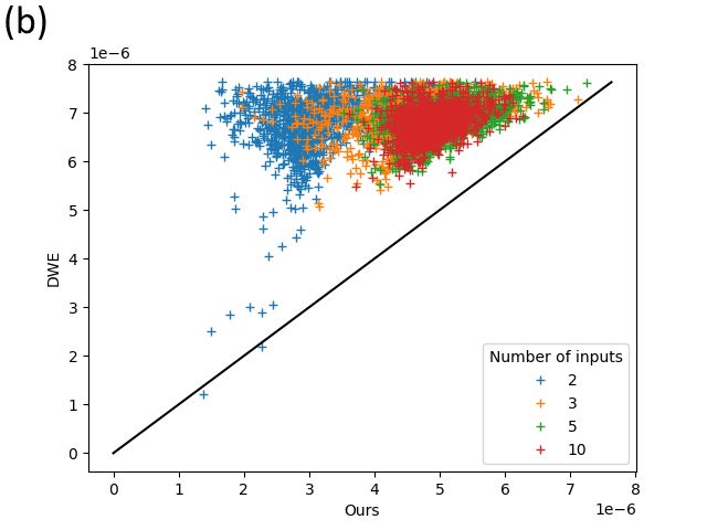
Figure 4: Approximation error of our model compared to the ones of DWE (version adapted to
handle 512×512 images), respectively measured in terms of (a) KL-Divergence and (b) L1 distance,
on images coming from our synthetic test dataset. Each one of the 1000 × 4 points corresponds
to a barycenter. The x-axis represents the error measured between the GeomLoss barycenter and
the barycenter predicted by our model while the y-axis represents the one between the GeomLoss
barycenter and the barycenter predicted by DWE. The color of a point associated to a barycenter
represents its number of inputs.
In Fig.4, we show a numerical comparison of approximation errors between our model and DWE
adapted to 512 × 512 images of our shape contours dataset, in terms of KL-divergence and L1
distance. Our results clearly show that our method is able to approximate more accurately the
Wasserstein barycenter on 512 × 512 input measures.
Finally, we study the limitations of the generalization of our network on the Coil20 dataset (Nane
et al., 1996), which consists of images of objects on a black background. In figure 7, we show the
interpolation of 2 cars ; additional results are available in appendix B, figure 11.
4.2 N- WAY BARYCENTERS
Even if our model has been trained using only barycenters computed from pairs of inputs, we can
apply it to predict barycenters of more than two measures. We display interpolations between re-
spectively three and five input measures in Fig.8, which surprisingly tends to show that our model
can generalize what it learned on pairs of inputs, at least partially. Additional results on Quick,
Draw! are also shown in appendix B, Fig. 12. A 100-way barycenter comparison can be found in
appendix Sec. B, Fig. 13.
7Under review as a conference paper at ICLR 2021
GeomLoss
Our Model
DWE
Figure 5: Interpolations between two 28×28 images from the Quick, Draw! dataset using Geomloss,
our model and the original Deep Wasserstein Embedding (DWE) method from (Courty et al., 2017).
Our model directly considers 512 × 512 inputs and its results are downsampled from 512 × 512 to
28 × 28.
GeomLoss
Our Model
DWE
Figure 6: Interpolations between two 512 × 512 images from the Quick, Draw! dataset using
Geomloss, our model and the Deep Wasserstein Embedding (DWE) method from (Courty et al.,
2017) adapted to handle 512 × 512 images.
Numerically when the number of inputs is greater than 2, our model also achieve to find better
approximations than the ones obtained with DWE, as shown in Fig. 4.
4.3 S PEED
In order to assess computational times, we obtain average running time over 1000 barycenter compu-
tations – on average, our model predicts barycenters of two images in 0.0092 seconds. We compare
the average speed of our model with GeomLoss in two different settings. The first one considers
the full 512 × 512 images – GeomLoss computes such barycenters in 1.41 seconds. The second
setting takes advantage of the sparsity of our images and only uses the 2D coordinates of the points
with non-zero mass – in this case, GeomLoss computes barycenters in 0.589 seconds. Our method
provides nearly 64x speedup compared with this last approach. In comparison, an exact barycenter
computation of two (sparse) measures using a network simplex (Bonneel et al., 2011) ranges from
4–80 seconds for typical shape contours images that contains few thousands of pixels carrying mass.
The time required to compute barycenters using the method of (Claici et al., 2018) depends on the
number of iterations, in our setting 100 iterations with the inputs shown in figure 3 require 37 hours
while 50 iterations are achieved in 14 hours. A 512 × 512 Radon barycenter (Bonneel et al., 2015)
requires 0.2 seconds for 720 projection directions, but remains far from the expected barycenter.
5 D ISCUSSION AND CONCLUSION
While our method produces good approximation of Wasserstein barycenters of n inputs, some
shapes are surprisingly difficult to handle. The barycenter of simple translated and scaled shapes
such as lines or ellipses should theoretically also be lines or ellipses, but are failure cases for our
model (Fig. 9), while more complex shapes are well handled (Fig. 8). In addition, we rely on a lin-
earized barycenter to train our network (Nader & Guennebaud, 2018; Wang et al., 2013; Moosmüller
& Cloninger, 2020; Mérigot et al., 2020), which incurs some error. This can be seen in appendix
Sec. C, Fig. 14. While using more iterations of gradient descent yields more accurate results and re-
moves this linearity, it also prevents easy combination and makes the dataset generation intractable.
8Under review as a conference paper at ICLR 2021
GeomLoss
Our Model
Figure 7: Interpolations between two 512 × 512 images from the Coil20 dataset (Nane et al., 1996)
using GeomLoss and our model trained with synthetic shape contours. In order to perform compu-
tations on the shapes and not on the background, mass has been inverted.
Inputs
GeomLoss (3)
Our Model (3)
GeomLoss (5)
Our Model (5)
Figure 8: Wasserstein barycenters of three inputs (top rows) and five inputs (bottom rows) from
Quick, Draw!, respectively computed with Geomloss and with our model trained with only pairs
from our synthetic training dataset. Barycentric weights are randomly chosen.
GeomLoss
Ours
2-circles 2-lines 5-circles 5-lines
Figure 9: Wasserstein barycenters of sets of lines or ellipses should result in lines (resp. ellipses).
Our prediction for two-way barycenters (here, with equal weights) of such shapes remains correct
(left). However, the predicted barycenter is highly distorted for 5-way barycenters of simple shapes
(right) although it remains plausible for more complex shapes (see Fig. 8).
Nevertheless, in many cases our DCNN is able to synthesize a barycenter from an arbitrary number
of inputs. The main strength of our approach lies in its capacity to be trained from only 2-inputs
barycenters examples and to generalize to any number of inputs. We showed that the results ex-
ceeded the ones obtained by explicit Wasserstein Embedding computation while having a very low
computation time. We hope our fast approach will accelerate the adoption of optimal transport in
machine learning applications.
9Under review as a conference paper at ICLR 2021
R EFERENCES
Brandon Amos, Lei Xu, and J Zico Kolter. Input convex neural networks. In International Confer-
ence on Machine Learning, pp. 146–155, 2017.
Alexandr Andoni, Piotr Indyk, and Robert Krauthgamer. Earth mover distance over high-
dimensional spaces. In SODA, volume 8, pp. 343–352, 2008.
Alexandr Andoni, Assaf Naor, and Ofer Neiman. Impossibility of sketching of the 3d transportation
metric with quadratic cost. In 43rd International Colloquium on Automata, Languages, and
Programming (ICALP 2016). Schloss Dagstuhl-Leibniz-Zentrum fuer Informatik, 2016.
Martin Arjovsky, Soumith Chintala, and Léon Bottou. Wasserstein gan, 2017.
Julio Backhoff-Veraguas, Joaquin Fontbona, Gonzalo Rios, and Felipe Tobar. Bayesian learning
with wasserstein barycenters. arXiv preprint arXiv:1805.10833, 2018.
Jérémie Bigot, Raúl Gouet, Thierry Klein, Alfredo López, et al. Geodesic pca in the wasserstein
space by convex pca. In Annales de l’Institut Henri Poincaré, Probabilités et Statistiques, vol-
ume 53, pp. 1–26. Institut Henri Poincaré, 2017.
Nicolas Bonneel, Michiel van de Panne, Sylvain Paris, and Wolfgang Heidrich. Displacement Inter-
polation Using Lagrangian Mass Transport. ACM Transactions on Graphics (SIGGRAPH ASIA
2011), 30(6), 2011.
Nicolas Bonneel, Julien Rabin, Gabriel Peyré, and Hanspeter Pfister. Sliced and radon wasserstein
barycenters of measures. Journal of Mathematical Imaging and Vision, 51(1):22–45, 2015.
Nicolas Bonneel, Gabriel Peyré, and Marco Cuturi. Wasserstein Barycentric Coordinates: His-
togram Regression Using Optimal Transport. ACM Transactions on Graphics (SIGGRAPH 2016),
35(4), 2016.
Harold C Burger, Christian J Schuler, and Stefan Harmeling. Image denoising: Can plain neural
networks compete with bm3d? In 2012 IEEE conference on computer vision and pattern recog-
nition, pp. 2392–2399. IEEE, 2012.
Sebastian Claici, Edward Chien, and Justin Solomon. Stochastic wasserstein barycenters. arXiv
preprint arXiv:1802.05757, 2018.
Nicolas Courty, Rémi Flamary, and Devis Tuia. Domain adaptation with regularized optimal
transport. In Joint European Conference on Machine Learning and Knowledge Discovery in
Databases, pp. 274–289. Springer, 2014.
Nicolas Courty, Rémi Flamary, and Mélanie Ducoffe. Learning wasserstein embeddings. arXiv
preprint arXiv:1710.07457, 2017.
Marco Cuturi. Sinkhorn distances: Lightspeed computation of optimal transport. In Advances in
neural information processing systems, pp. 2292–2300, 2013.
Pierre Dognin, Igor Melnyk, Youssef Mroueh, Jerret Ross, Cicero Dos Santos, and Tom Sercu.
Wasserstein barycenter model ensembling. arXiv preprint arXiv:1902.04999, 2019.
G Domazakis, D Drivaliaris, S Koukoulas, G Papayiannis, A Tsekrekos, and A Yannacopoulos.
Clustering measure-valued data with wasserstein barycenters. arXiv preprint arXiv:1912.11801,
2020.
Jiaojiao Fan, Amirhossein Taghvaei, and Yongxin Chen. Scalable computations of wasserstein
barycenter via input convex neural networks. arXiv preprint arXiv:2007.04462, 2020.
Jean Feydy. Geometric loss functions between sampled measures, images and volumes, 2019. URL
https://www.kernel-operations.io/geomloss/.
Jean Feydy, Thibault Séjourné, François-Xavier Vialard, Shun-Ichi Amari, Alain Trouvé, and
Gabriel Peyré. Interpolating between optimal transport and mmd using sinkhorn divergences.
arXiv preprint arXiv:1810.08278, 2018.
10Under review as a conference paper at ICLR 2021
Jean Feydy, Pierre Roussillon, Alain Trouvé, and Pietro Gori. Fast and scalable optimal transport
for brain tractograms. In International Conference on Medical Image Computing and Computer-
Assisted Intervention, pp. 636–644. Springer, 2019.
Charlie Frogner, Farzaneh Mirzazadeh, and Justin Solomon. Learning embeddings into entropic
wasserstein spaces. arXiv preprint arXiv:1905.03329, 2019.
Aude Genevay, Gabriel Peyré, and Marco Cuturi. Learning generative models with sinkhorn diver-
gences. arXiv preprint arXiv:1706.00292, 2017.
Inc. Google. The quick, draw! dataset, 2020. URL https://github.com/
googlecreativelab/quickdraw-dataset.
Matthieu Heitz, Nicolas Bonneel, David Coeurjolly, Marco Cuturi, and Gabriel Peyré. Ground
Metric Learning on Graphs. Technical Report arXiv:1911.03117, November 2019.
L Kantorovich. On the transfer of masses (in russian). In Doklady Akademii Nauk, volume 37, pp.
227–229, 1942.
Wei-Sheng Lai, Jia-Bin Huang, Narendra Ahuja, and Ming-Hsuan Yang. Deep laplacian pyramid
networks for fast and accurate super-resolution. In Proceedings of the IEEE conference on com-
puter vision and pattern recognition, pp. 624–632, 2017.
Christian Ledig, Lucas Theis, Ferenc Huszár, Jose Caballero, Andrew Cunningham, Alejandro
Acosta, Andrew Aitken, Alykhan Tejani, Johannes Totz, Zehan Wang, et al. Photo-realistic sin-
gle image super-resolution using a generative adversarial network. In Proceedings of the IEEE
conference on computer vision and pattern recognition, pp. 4681–4690, 2017.
Stamatios Lefkimmiatis. Non-local color image denoising with convolutional neural networks. In
Proceedings of the IEEE Conference on Computer Vision and Pattern Recognition, pp. 3587–
3596, 2017.
Guilin Liu, Fitsum A Reda, Kevin J Shih, Ting-Chun Wang, Andrew Tao, and Bryan Catanzaro.
Image inpainting for irregular holes using partial convolutions. In Proceedings of the European
Conference on Computer Vision (ECCV), pp. 85–100, 2018.
Antoine Liutkus, Umut Simsekli, Szymon Majewski, Alain Durmus, and Fabian-Robert Stöter.
Sliced-wasserstein flows: Nonparametric generative modeling via optimal transport and diffu-
sions. In International Conference on Machine Learning, pp. 4104–4113. PMLR, 2019.
Ilya Loshchilov and Frank Hutter. Sgdr: Stochastic gradient descent with warm restarts. arXiv
preprint arXiv:1608.03983, 2016.
Quentin Mérigot, Alex Delalande, and Frederic Chazal. Quantitative stability of optimal transport
maps and linearization of the 2-wasserstein space. volume 108 of Proceedings of Machine Learn-
ing Research, pp. 3186–3196, 2020.
Alberto Maria Metelli, Amarildo Likmeta, and Marcello Restelli. Propagating uncertainty in rein-
forcement learning via wasserstein barycenters. In Advances in Neural Information Processing
Systems, pp. 4333–4345, 2019.
Liang Mi, Wen Zhang, Xianfeng Gu, and Yalin Wang. Variational Wasserstein clustering. In Pro-
ceedings of the European Conference on Computer Vision (ECCV), pp. 322–337, 2018.
Caroline Moosmüller and Alexander Cloninger. Linear optimal transport embedding: Provable fast
wasserstein distance computation and classification for nonlinear problems, 2020.
Georges Nader and Gael Guennebaud. Instant transport maps on 2d grids. ACM Trans. Graph., 37
(6), 2018. ISSN 0730-0301.
SA Nane, SK Nayar, and H Murase. Columbia object image library: Coil-20. Dept. Comp. Sci.,
Columbia University, New York, Tech. Rep, 1996.
Gabriel Peyré, Marco Cuturi, et al. Computational optimal transport. Foundations and Trends® in
Machine Learning, 11(5-6):355–607, 2019.
11Under review as a conference paper at ICLR 2021
Antoine Rolet, Marco Cuturi, and Gabriel Peyré. Fast dictionary learning with a smoothed wasser-
stein loss. In Artificial Intelligence and Statistics, pp. 630–638, 2016.
Olaf Ronneberger, Philipp Fischer, and Thomas Brox. U-net: Convolutional networks for biomedi-
cal image segmentation. In International Conference on Medical image computing and computer-
assisted intervention, pp. 234–241. Springer, 2015.
Morgan A. Schmitz, Matthieu Heitz, Nicolas Bonneel, Fred Maurice Ngolè Mboula, David Coeur-
jolly, Marco Cuturi, Gabriel Peyré, and Jean-Luc Starck. Wasserstein dictionary learning: Op-
timal transport-based unsupervised non-linear dictionary learning. SIAM Journal on Imaging
Sciences, 11(1), 2018.
Bernhard Schmitzer. Stabilized sparse scaling algorithms for entropy regularized transport problems.
SIAM Journal on Scientific Computing, 41(3):A1443–A1481, 2019.
Justin Solomon, Fernando De Goes, Gabriel Peyré, Marco Cuturi, Adrian Butscher, Andy Nguyen,
Tao Du, and Leonidas Guibas. Convolutional wasserstein distances: Efficient optimal transporta-
tion on geometric domains. ACM Transactions on Graphics (TOG), 34(4):1–11, 2015.
Ying Tai, Jian Yang, and Xiaoming Liu. Image super-resolution via deep recursive residual network.
In Proceedings of the IEEE conference on computer vision and pattern recognition, pp. 3147–
3155, 2017.
Dmitry Ulyanov, Andrea Vedaldi, and Victor Lempitsky. Instance normalization: The missing in-
gredient for fast stylization. arXiv preprint arXiv:1607.08022, 2016.
Dmitry Ulyanov, Andrea Vedaldi, and Victor Lempitsky. Deep image prior. In Proceedings of the
IEEE Conference on Computer Vision and Pattern Recognition, pp. 9446–9454, 2018.
Wei Wang, Dejan Slepčev, Saurav Basu, John A Ozolek, and Gustavo K Rohde. A linear optimal
transportation framework for quantifying and visualizing variations in sets of images. Interna-
tional journal of computer vision, 101(2):254–269, 2013.
Junyuan Xie, Linli Xu, and Enhong Chen. Image denoising and inpainting with deep neural net-
works. In Advances in neural information processing systems, pp. 341–349, 2012.
Raymond A Yeh, Chen Chen, Teck Yian Lim, Alexander G Schwing, Mark Hasegawa-Johnson, and
Minh N Do. Semantic image inpainting with deep generative models. In Proceedings of the IEEE
conference on computer vision and pattern recognition, pp. 5485–5493, 2017.
A L EARNING S TRATEGY
Instead of using a fixed learning rate or a decreasing learning rate, we choose a learning rate schedule
with warm restart as proposed by Loshchilov & Hutter (2016). The learning schedule is shown in
Figure 10: the learning rate decreased and is periodically restarted to its initial value, the period
increasing as the number of epochs grows. This schedule was chosen after comparing with stepwise
schedules or constant learning rates and yielded better convergence in practice.
B A DDITIONAL RESULTS
To better show the limitations of the generalization of our network when the number of inputs is 2,
we show additional interpolations between 2 objects from the Coil20 in figure 11. There are two
reasons for these bad results: first, our model is trained in synthetic shape contours and do not look
at all like these images. Furthermore, the cup image seem to be even more challenging than the
car image for our network, and our best explanation for this failure is that the cup covers almost
the whole image. We provide additional experiments showing barycenters of 5 sketches on Figure
12. The weights evolve linearly inside the pentagon. As a stress test, we also show a barycenter of
100 cats with equal weights in Fig. 13 and compare it with a barycenter computed with GeomLoss.
While both results recover more or less the global shape of the cat, details are clearly lost and our
result looks much smoother.
12Under review as a conference paper at ICLR 2021
Figure 10: Learning rate schedule used to train our models, following the SGDR method described
by Loshchilov & Hutter (2016). Our training runs for a total of 31 epochs. Compared to a constant
learning rate or to stepwise schedules, SGDR has empirically shown a better convergence in our
context.
GeomLoss
Our Model
Figure 11: Additional interpolations between two 512 × 512 images from the Coil20 dataset using
GeomLoss and our model. Mass is inverted.
C L INEARIZED BARYCENTERS
Fig. 14 shows the error introduced by using a linearized version of Wasserstein barycenters (Nader
& Guennebaud, 2018; Wang et al., 2013; Moosmüller & Cloninger, 2020; Mérigot et al., 2020). Our
predicted barycenters reflect this error.
13Under review as a conference paper at ICLR 2021
Figure 12: Interpolations between 5 inputs from Quick, Draw!, shown as pentagons. Left pentagon
corresponds to GeomLoss barycenters while the right one shows predictions of our model trained
on our synthetic dataset.
14Under review as a conference paper at ICLR 2021
GeomLoss Our DCNN
Figure 13: Stress test. We predict a barycenter of 100 cats of the QuickDraw dataset, with equal
weights.
input 1 input 2 Geomloss (1) Geomloss (10) Ours
λ1 = 0.4382 λ2 = 0.5618
Figure 14: Wasserstein barycenter computed from a pair of inputs respectively using Geomloss with
only one descent step, Geomloss with 10 descent steps and using our model trained on our synthetic
training dataset.
15You can also read