Distributed Charge Models of Liquid Methane and Ethane for Dielectric Effects and Solvation
←
→
Page content transcription
If your browser does not render page correctly, please read the page content below
Distributed Charge Models of Liquid Methane and Ethane for Dielectric
                                                   Effects and Solvation
                                                            Atul C. Thakur1 and Richard C. Remsing1, a)
                                                            Department of Chemistry and Chemical Biology, Rutgers University, Piscataway,
                                                            NJ 08854
                                                            Liquid hydrocarbons are often modeled with fixed, symmetric, atom-centered charge distributions and
                                                            Lennard-Jones interaction potentials that reproduce many properties of the bulk liquid. While useful for
                                                            a wide variety of applications, such models cannot capture dielectric effects important in solvation, self-
                                                            assembly, and reactivity. The dielectric constants of hydrocarbons, such as methane and ethane, physically
arXiv:2011.12481v1 [physics.chem-ph] 25 Nov 2020

                                                            arise from electronic polarization fluctuations induced by the fluctuating liquid environment. In this work,
                                                            we present non-polarizable, fixed-charge models of methane and ethane that break the charge symmetry of
                                                            the molecule to create fixed molecular dipoles, the fluctuations of which reproduce the experimental dielec-
                                                            tric constant. These models can be considered a mean-field-like approximation that can be used to include
                                                            dielectric effects in large-scale molecular simulations of polar and charged molecules in liquid methane and
                                                            ethane. We further demonstrate that solvation of model solutes in these fixed-dipole models improve upon
                                                            dipole-free models.

                                                   I.   INTRODUCTION                                             fixed charge models of methane and ethane cannot read-
                                                                                                                 ily describe dielectric effects. Methane and ethane do
                                                     Understanding the liquid-state properties of hydrocar-      not have a permanent dipole moment, due to symmetry,
                                                   bons is important for applications in the petrochemi-         and consequently any symmetric and rigid fixed charge
                                                   cal industry1–3 , as well as their use as solvents for syn-   model yields a dielectric constant of unity. Therefore,
                                                   thesis and separations. Liquid hydrocarbons have also         these standard models cannot properly describe the re-
                                                   garnered attention in the past as models for simple,          sponse of hydrocarbon solvents to polar and charged so-
                                                   non-associating liquids4,5 . Interest in the simplest of      lutes.
                                                   these liquids has been reinvigorated by the discovery of         Physically, the dielectric responses of methane and
                                                   methane/ethane lakes on the cold (∼ 94 K) surface of the      ethane arise from their polarizabilities. The relevant
                                                   Saturnian moon Titan6–13 . The existence of liquid reser-     dipole fluctuations can be accounted for by polarizable
                                                   voirs on Titan’s surface, combined with its rich atmo-        and ab initio models30–35 . However, polarizable models
                                                   spheric chemistry, has led many to hypothesize that the       can be difficult to parameterize and are more expensive
                                                   hydrocarbon lakes could harbor prebiotic chemistry and        than the fixed charge models discussed above. An in-
                                                   even non-aqueous life14–18 . However, any such chemistry      termediate class of models with fixed charges and the
                                                   would be vastly different than similar processes in aque-     ability to describe dielectric effects was introduced by
                                                   ous environments, and a fundamental, molecular-scale          Fennell et al., referred to as dielectric corrected (DC)
                                                   understanding is necessary, beginning with characteriz-       models36 . For symmetric molecules without a perma-
                                                   ing solvation in methane and ethane15,19–23 . Such a mi-      nent dipole moment, a DC model breaks the molecular
                                                   croscopic picture of cryogenic hydrocarbon solutions can      charge symmetry to create a fixed dipole moment, which
                                                   be provided by molecular simulations, but there remains       is parameterized to reproduce the dielectric constant of
                                                   a need to make these simulations efficient and predictive.    the liquid phase.
                                                     One difficulty presented by modeling liquid hydro-             In this work, we present DC models for liquid methane
                                                   carbons is a description of their dielectric properties.      and ethane at Titan surface conditions. In addition to
                                                   United-atom models combine the carbon and hydrogen            describing dielectric constants of the pure liquids, we
                                                   atoms into single sites with intermolecular interactions      find that the DC models provide a good description of
                                                   described by Lennard-Jones (LJ) potentials and can-           the dielectric constant of methane/ethane mixtures. We
                                                   not describe dielectric effects by construction24 . Most      also demonstrate that these models yield structure and
                                                   atomically-detailed molecular models of hydrocarbons          dynamics in good agreement with the original, dipole-
                                                   describe the intermolecular interactions through atom-        free models, such that the DC models provide a reason-
                                                   based LJ and electrostatic interactions, with the latter      able description of the two bulk liquids. We then turn
                                                   achieved by assigning a fixed set of point-charges to each    to the solvation of model solutes. We first investigate
                                                   molecule25–27 . These and similar models have been rea-       hard sphere solvation and the corresponding liquid den-
                                                   sonably successful, and can adequately describe liquid        sity fluctuations, demonstrating that all models studied
                                                   hydrocarbon structure and many thermodynamic prop-            here provide good descriptions of apolar solvation. Then,
                                                   erties, including at Titan conditions28,29 . However, these   we investigate charging a hard sphere as a model ionic
                                                                                                                 solute. In this case, the DC models provide very different
                                                                                                                 results than the symmetric, dipole-free models, because
                                                   a) rick.remsing@rutgers.edu
                                                                                                                 the DC models exhibit a larger dielectric response. Our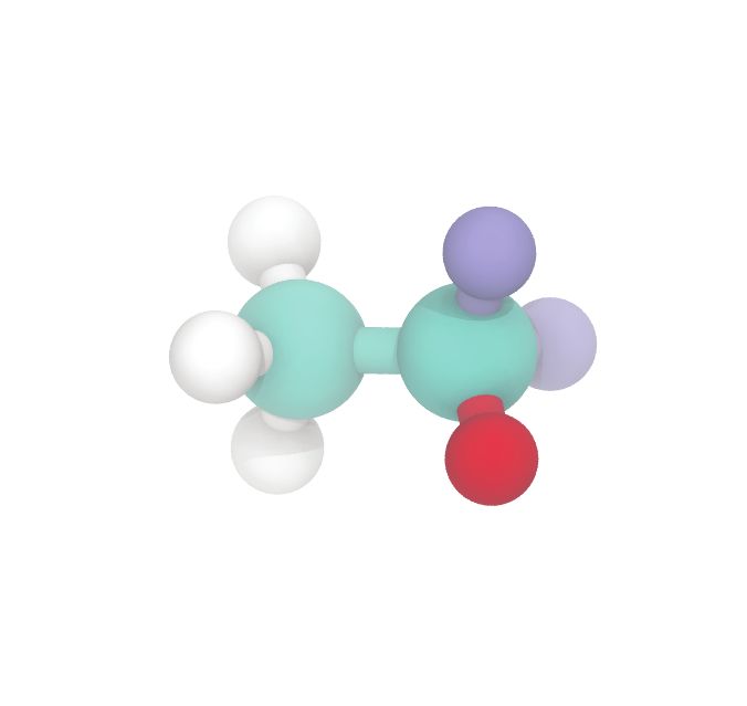
2
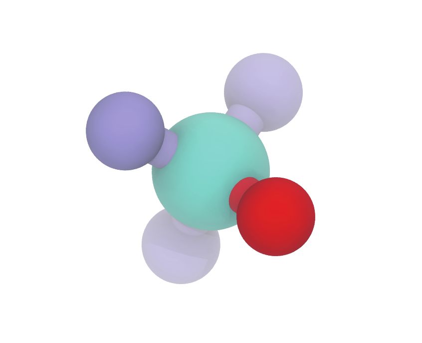
(a) (b) (c)
q+δ/3 q q
q+δ/2 q
q+δ/3
-4q -3q -3q q+δ/2 q -3q+δ -3q-δ q
q
q-δ
q q-δ q q
q+δ/3
FIG. 1. Schematics of the charge distributions for (a) the DC model of methane and the (b) DC and (c) DC2 models of
ethane.
results suggest that DC models can be used in place of electrostatic interactions were evaluated using the parti-
traditional dipole-free models to accurately predict sol- cle mesh Ewald method44 in conjunction with the correc-
vation thermodynamics of polar and charged species in tion of Yeh and Berkowitz for slab-like systems49 , and all
hydrocarbon solutions, like those on the surface of Titan. other simulation parameters followed those of the bulk
systems.
II. SIMULATION DETAILS
III. STATIC DIPOLAR CHARGE DISTRIBUTIONS CAN
All simulations were performed with GROMACS REPRODUCE THE DIELECTRIC CONSTANT
202037–39 . Simulations of the pure liquid methane and
ethane were performed with 697 molecules, and mixture Due to symmetry, both methane and ethane do not
simulations were performed with 697 molecules of one have static molecular dipole moments, so that the di-
liquid and 299 molecules of the other. After constructing electric constant is determined by electronic polarization
the simulation cells and performing an energy minimiza- fluctuations. Here, we develop models with fixed, effec-
tion, the systems were equilibrated for 1 ns in the canoni- tive dipole moments — using point charges distributed
cal ensemble, followed by equilibration of at least 10 ns in over the molecular sites — that can reproduce the ex-
the isothermal-isobaric (NPT) ensemble. Statistics were perimental dielectric constant of each liquid. This ap-
gathered over production runs of at least 50 ns in length proach can be considered a mean-field-like approxima-
in the NPT ensemble. A constant temperature of 94 K tion to the polarization fluctuations and is inspired by
was maintained using a Nosé-Hoover thermostat40,41 and the distributed-dipole DC models of Fennell et al.36 .
a constant pressure of 1 bar was maintained using an We tune the fixed point charges on atomic sites accord-
Andersen-Parrinello-Rahman barostat42,43 . Short-range ing to the schemes in Fig. 1, where dipoles are created
interactions (LJ and Coulomb) were truncated at 1 nm, using two parameters: a charge q and a shift parameter
with long-range corrections applied for the LJ contri- δ. Ethane presents more freedom in the choice of charge
bution to the energy and pressure. Long-range electro- distribution, and so we parameterize two models: DC
static interactions were evaluated using the particle mesh and DC2. The DC ethane model has a charge distribu-
Ewald method44 . All C-H bond lengths were constrained tion similar to the DC methane model, while the DC2
using the LINCS algorthim45 . All bond, angle, and LJ model creates a permanent dipole moment using the car-
parameters were taken from the OPLS force field26 , to bon atoms only. The magnitudes of q and δ are optimized
which we compare the results of the DC models. to match the experimental dielectric constants, and we
In order to simulate a hard-sphere-like solute with a find q = δ yields good results for the DC models. The
radius of 3 Å in methane and ethane, we created a non- resulting parameters are listed in Tables I and II, along
interacting dummy particle, fixed at the center of the with the dielectric constants and bulk densities of those
box, and we biased the coordination number of this parti- models, where the dielectric constants were determined
cle with a harmonic potential using PLUMED46 . For the according to
harmonic potential U (Ñ ) = κ/2(Ñ − Ñ ∗ )2 , where Ñ is a
smoothed variant of the coordination number necessary 4πβ
ε=1+ (δM)2 , (1)
for biasing47,48 , we set κ = 5 kJ/mol and Ñ ∗ = −20 in 3 hV i
order to exclude all solvent molecules from within 3 Å of
the solute particle. The biasing potential was applied to where β −1 = kB T is the product of Boltzmann’s con-
solvent carbon atoms only. Simulations of the methane stant and the temperature, h· · · i indicates an ensem-
liquid-vapor interface were performed in the canonical ble average, V is the volume of the simulation cell,
ensemble using a Nosé-Hoover thermostat40,41 . A liquid δM = M − hMi, and M is the total dipole moment
slab was created by elongating the z-axis of an equili- of the system. The running average of ε is shown in
brated bulk simulation by a factor of three. Long-range Fig. 2 for all models studied. The dielectric constants of3
TABLE II. Charge, q, shift parameter, δ, (e0 ) as de-
fined in Fig. 1, and predicted dielectric constants and den-
sities (kg/m3 ) for the ethane models studied here. Experi-
mental dielectric constants53,55 and densities54 are also listed.
(a) Error estimates are listed in parentheses.
Model q δ ε ρB
OPLS 0.06 0.0 1.0090 (0.0001) 668.38 (0.06)
DC 0.0576 0.0576 1.95 (0.01) 664.58 (0.16)
(b) DC2 0.06 0.06 1.94 (0.01) 663.46 (0.08)
Exp. − − 1.94 647.65
2
FIG. 2. Running averages of the dielectric constant in the
1.9
(a) methane and (b) ethane models studied here, shown for
the first 25 ns of a 50 ns trajectory.
1.8
ε
DC
1.7 DC2
TABLE I. Charge, q, shift parameter, δ, (e0 ) as defined
in Fig. 1, and predicted dielectric constants and densi-
ties (kg/m3 ) for the methane models studied here. Experi- Exp.
mental dielectric constants52,53 and densities54 are also listed. Oster
Error estimates are listed in parentheses.
1.6 0 0.2 0.4 0.6 0.8 1
Model
OPLS
q
0.06
δ
0.0
ε
1.006 (0.001)
ρB
465.64 (0.2)
x
DC 0.0462 0.0462 1.654 (0.002) 458.51 (0.1)
Exp. − − 1.67 447.04 FIG. 3. Dielectric constant of methane-ethane mixtures as a
function of the methane mole fraction, x, determined via sim-
ulation with the DC models developed here and determined
the DC models are in good agreement with those deter- by experiments53 . Also shown are the predictions from Os-
mined experimentally. The OPLS models have dielectric ter’s formula56 , Eq. 2, with the shaded region indicating the
constants close to unity, with deviations coming from in- range of predictions consistent with the error bars.
tramolecular H-C-H and H-C-C angle fluctuations. The
bulk densities are also listed in Tables I and II, showing
that the density is only slightly lowered in the DC mod- show the predictions of Oster’s formula for the dielectric
els, in comparison to the OPLS models, in agreement constant of mixtures56 ,
with previous work that showed that reasonable atomic
ε(x) − 1 X ρB (x) εi − 1
charges have little impact on the thermodynamic proper- = xi , (2)
ties of liquid alkanes50,51 . We additionally note that this ε(x) + 2 i
ρB,i εi + 2
lowering of the density brings the DC models in closer
agreement with experiments. where xi is the mole fraction of component i, ρB (x) is the
Although the DC models were parameterized to match number density of the mixture x, ρB,i is the bulk density
the dielectric constant of pure liquid methane and ethane, of pure component i, and εi is the dielectric constant of
they can also make reasonable predictions for the dielec- pure component i. To determine ε for intermediate mole
tric constant of their mixtures. To demonstrate this, we fractions, we fit the density to a quadratic function of x
performed simulations of methane-ethane mixtures with and use this as input to Eq. 2.
methane mole fractions of x = 0.3 and x = 0.7. The di- The concentration-dependence of the dielectric con-
electric constants as a function of x are shown in Fig. 3, stant, shown in Fig. 3, is in good agreement with exper-
along with available experimental data points. We also imental results and the predictions of Eq. 2. The Oster
equation is anticipated to be accurate for methane-ethane4
(a) (b) (a) (b)
FIG. 4. Radial distribution functions, g(r), for C-C, H-H, FIG. 5. Mean-squared displacement (MSD) as a function of
and C-H (intermolecular) correlations in liquid (a) methane time for the (a) methane and (b) ethane models studied here.
and (b) ethane. Lines indicate g(r) obtained using the dipole-
free, OPLS model, and those for the DC models are shown
with data points. The H-H and C-H results are shifted verti-
cally by 0.5 and 1, respectively.
mixtures, because it is an extension of the Clausius-
Mossotti formula57 , which has been shown to be accu- (a) (b)
rate for pure methane and ethane liquids53,55 . The good
agreement among the predictions of the dipole-free mod-
els, Eq. 2, and experiments suggests that these models
can be accurately used to simulate dielectric effects at a
range of concentrations, including the ranges anticipated
FIG. 6. Rotational time correlation functions, C2 (t), for (a)
for Titan’s lakes. methane and (b) ethane models studied here. The methane
C2 (t) quantifies the rotation of the C-H bond vector, while
that for ethane quantifies the C-C bond rotation.
IV. LIQUID-STATE STRUCTURE AND DYNAMICS
The OPLS models of methane and ethane yield accu- D, through the Einstein relation, 6Dt = limt→∞ MSD(t),
rate predictions for the structure and dynamics of these such that similar MSDs in two systems imply similar dif-
liquids. In this section, we demonstrate that creating the fusion coefficients. The MSDs are shown in Fig. 5 for
DC models of methane and ethane leaves the structure all systems under study. The dynamics of the DC mod-
and dynamics essentially unchanged. els are slightly faster than the original OPLS models,
We characterize the structure of liquid methane and which can be attributed in part to the slightly lower den-
liquid ethane through site-site pair distribution func- sity of the DC models. The faster dynamics of the DC
tions, gαγ (r), where α and γ represent atomic sites. models is reflected in the diffusion coefficients, which we
The carbon-carbon (CC), hydrogen-hydrogen (HH), and obtained by linear fitting the long-time behavior of the
carbon-hydrogen (CH) pair distribution functions of liq- MSD to 6Dt + c. This yields diffusion coefficients of
uid methane and ethane are shown in Fig. 4 for the DOPLS ≈ 4.1 × 10⁻⁵ cm2 /s and DDC ≈ 4.7 × 10⁻⁵ cm2 /s
original and DC models. The various gαγ (r) are essen- for the OPLS and DC models of methane, respectively.
tially identical for the two models. This illustrates that Both models predict diffusion coefficients that are slightly
the small change in charge distributions necessary to ob- larger than that obtained at T = 95.94 K by Oosting and
tain the experimental dielectric constant does not signif- Trappeniers at coexistence58 , Dexp = 3.01 × 10⁻⁵ cm2 /s.
icantly change the structure of the bulk liquid, resulting The analogous diffusion coefficients for the ethane
in fixed-charge models with accurate structure and di- models are DOPLS ≈ 0.30 × 10⁻⁵ cm2 /s and DDC ≈
electric properties. The DC2 model yields gαγ (r) indis- 0.35 × 10⁻⁵ cm2 /s, respectively. This further supports
tinguishable from the OPLS and DC models and are not that the DC models diffuse slightly faster than the dipole-
shown for clarity. free models, and we also attribute this small difference
To the extent that liquid structure determines dy- to the slightly lower density of the DC system at the
namic properties in equilibrium, the above results suggest same pressure. In this case, both models exhibit slightly
that the DC models should yield liquid dynamics similar slower diffusion than that determined experimentally,
to the original dipole-free models. To characterize the Dexp ≈ 0.8 × 10⁻⁵ cm2 /s, by Gaven, Stockmayer, and
single-particle translational dynamics of each liquid, we Waugh at approximately 98 K59 .
compute the mean-squared displacement (MSD) in each While the addition of a permanent dipole only slightly
system. The MSD is related to the diffusion coefficient, influences translational diffusion, one might imagine that5
it could impact rotational motion. Therefore, we addi- (a) (b)
tionally examined single-molecule rotational dynamics by
computing the rotational correlation function
C2 (t) = hP2 (n(t) · n(0))i , (3)
where n(t) is a C-H bond vector in the case of methane
and the C-C bond vector in the case of ethane at time
t and P2 (x) is the second order Legendre polynomial.
These rotational correlation functions are shown in Fig. 6
for the methane and ethane models studied here. For
methane, C2 (t) is nearly identical for the OPLS and
DC model, illustrating that the addition of a permanent
dipole moment does not significantly affect rotational
motion in the liquid. Exponential fits to the long-time
decay of C2 (t) (0.4 ps to 2 ps) yield correlation times of
τOPLS ≈ 0.26 ps and τDC ≈ 0.27 ps, further illustrating (c) (d)
that the DC minimally perturbs the dynamics of liquid
methane. These correlation times are in good agreement
with that of approximately 0.2 ps determined experimen-
tally through Raman spectroscopy60,61 .
For ethane, C2 (t) decays slightly faster in the DC FIG. 7. (a,b) Probability distribution, Pv (N ), of the num-
and DC2 models than that for the OPLS model. The ber of solvent molecules, N , within a spherical volume, v,
long-time decay of C2 (t) for ethane (5 ps to 30 ps) is for (a) methane and (b) ethane models. From left to right,
fit well with a bi-exponential, which we integrate to the spherical volumes have radii of RHS = 2 Å, RHS = 3 Å,
find the correlation time. This yields τOPLS ≈ 3.48 ps, and RHS = 4 Å. OPLS model results are shown as circles,
τDC ≈ 3.08 ps, and τDC2 ≈ 3.03 ps. Performing the same DC model results are shown as diamonds. Solid lines corre-
fit on the experimental correlation function62 yields a cor- spond the predictions of Eq. 4. (c,d) Hard sphere solvation
relation time of 2.9 ps, in good agreement with the DC free energy, ∆µv , as of function of the solute radius for both
model predictions. The addition of a permanent dipole models (points), as well as their respective Gaussian approx-
imations (thin solid/dashed lines). The thick gray line in (c)
moment in the DC models slightly speeds up the rota-
is the prediction of the theory of Chen and Weeks (CW)70 ,
tional dynamics of liquid ethane, in addition to trans- Equation 9.
lational diffusion. While this can in part be attributed
to a slightly lower density, dynamical dielectric response,
which involves rotational motion, is inversely related to where hN iv = ρB v is the average number of solvent
the dielectric constant, i.e. higher dielectric constant liq- molecules in v at a bulk density ρB . The variance in
uids have faster dielectric response when all other prop- the number fluctuations, (δN )2 v , is given by
erties are the same63 . Thus, it may be expected that the
DC models presented here will have slightly faster ro-
Z Z
tational dynamics through their connection to dielectric (δN ) v = dr dr0 hδρ(r)δρ(r0 )i ,
2
(5)
v v
relaxation.
To summarize, the DC models yield a reasonable de- where the bulk density-density correlation function is
scription of the structure and dynamics of liquid methane
and ethane, while also providing an accurate representa- hδρ(r)δρ(r0 )i = ρB ωCC (|r − r0 |) + ρ2B [gCC (|r − r0 |) − 1]
tion of the static dielectric constant of each liquid. (6)
and ωCC (r) is the carbon-carbon intramolecular pair
correlation function, equal to a delta function for
V. DENSITY FLUCTUATIONS AND HARD SPHERE methane67–69 . Therefore, if Pv (N ) is Gaussian, we would
SOLVATION expect the OPLS and DC models to yield equivalent
distributions, because both yield liquids with the same
We now evaluate how altering the charge distribution structure.
of the methane and ethane models impact solvation of The computed distributions, Pv (N ), are shown in
small apolar solutes. To do so, we quantify density fluc- Fig. 7a,b for liquid methane and ethane models and
tuations in each liquid through the probability distribu- representative spherical probe volumes, where N cor-
tion, Pv (N ), of observing N heavy atoms in a spherical responds to the number of carbon atoms in the probe
probe volume, v. For small v, Pv (N ) is expected to follow volume. For small v, we find that the distributions are
Gaussian statistics47,64–66 . In this limit, approximately Gaussian, and that the dipole-free and
DC models yield equivalent distributions. This is ex-
(N − hN iv )2
1 pected based on the discussion above; both sets of mod-
Pv (N ) = p exp − , (4)
2π h(δN )2 iv 2 h(δN )2 iv els produce the same gαγ (r) and therefore the same den-6
sity fluctuations. However, for larger volumes, close to roughly where gCC (r) becomes non-zero. The predic-
RHS ≈ 3 Å and larger, Pv (0) is overestimated by the tions of Eq. 9 are shown as a gray solid line in Fig. 7c and
Gaussian prediction. agree well with the simulation results for all values of RHS
The solvation free energy of a hard sphere of volume v, studied here. For larger RHS values, long-range solvent-
∆µv , can be obtained from the quantification of density solvent interactions become increasingly important, but
fluctuations using Widom’s particle insertion these can be accounted for using recent theoretical ap-
proaches77 . These results suggest that small-scale den-
β∆µv = − ln Pv (0) (7) sity fluctuations in atomistic models of liquid methane
ρ2B v 2 1 are analogous to those of their hard sphere counterparts,
ln 2π (δN )2 v ,
≈ + (8) and solvation of small apolar solutes can be described
2 h(δN )2 iv 2
within this level of approximation with reasonable accu-
where the second line is obtained using the Gaussian ap- racy. We expect that liquid ethane will follow similar
proximation to Pv (N ) in Eq. 4. Hard sphere solvation principles — apolar solvation can be described using a
free energies as a function of solute size are shown in hard diatomic fluid — and we leave the extension of the
Fig. 7c,d for liquid methane and ethane, along with the CW theory70 and complementary approaches67,68,78,79 to
predictions of Eq. 8. The free energies are in agreement treat diatomic solvents with varying bond length for fu-
for the two sets of charges, suggesting that the DC mod- ture work.
els can be used for studying the solvation of apolar so-
lutes. Moreover, the Gaussian approximation holds for
hard sphere radii less than about 2.75 Å, suggesting that VI. FREE ENERGY OF HARD SPHERE CHARGING IN
Eq. 4 can be used to predict solvation free energies in this LIQUID METHANE
range of solute sizes. Above this size, the Gaussian ap-
proximation underestimates the free energy, as expected The results above demonstrate that the structure and
by the overestimate of Pv (0) by the Gaussian approxi- dynamics of liquid methane and ethane, and conse-
mation in Fig. 7a,b. quently apolar solvation in these two solvents, are es-
These deviations from Gaussianity at low N are also sentially unaltered by introducing a small, fixed dipole
observed for hard sphere fluids66,71,72 . Within the per- moment on each molecule. Thus, the DC models can
spective of Weeks-Chandler-Andersen (WCA) theory, the describe the properties of liquid methane and ethane as
pair correlations in liquid methane and ethane are deter- well as earlier dipole-free fixed charge models, with the
mined mainly by the short-range, rapidly-varying repul- additional advantage of providing a reasonable descrip-
sive cores of the molecular sites, while the slowly-varying, tion of the static dielectric constant. As an example of
long-range attractions provide essentially a uniform back- where dielectric response is significant and therefore dif-
ground potential67,68,73–75 . Therefore, the molecular liq- fers between the two models, we examine the process of
uid can be accurately approximated by its purely short- charging hard sphere solutes in liquid methane.
ranged counterpart at the same bulk density. WCA also We consider inserting a point charge at the center of a
showed that the correlations within this short-ranged hard sphere of radius RHS = 3 Å in solution and evalu-
reference system can be further approximated by those ate the corresponding free energies of charging the solute
of an appropriately-chosen hard sphere reference sol- to a charge Q. We obtain the charging free energy by
vent73,75,76 . Within this level of approximation, we can linearly coupling the charge to a parameter λ, such that
approximate the hard sphere solvation free energy, ∆µv , λ = 0 corresponds to the uncharged hard sphere and
by that in an appropriate hard sphere reference fluid. λ = 1 indicates the fully charged solute. Through ther-
An analytic expression for this solvation free energy was modynamic integration, the charging free energy is given
derived by Chen and Weeks (CW)70 , by63,80,81
η(2 − 7η + 11η 2 ) Z 1 Z Z
ρQ (r)ρqλ (r0 )
β∆µCW
v =− − ln(1 − η) c
∆G (Q) = dλ dr dr0 , (10)
2(1 − η)3 0 |r − r0 |
18η 3 RHS 18η 2 (1 + η) RHS
2
+ − where
(1 − η)3 σ (1 − η)3 σ 2
2 3
8η(1 + η + η ) RHS ρqλ (r) = ρq (r; R) (11)
+ , (9) λ
(1 − η)3 σ3
h· · · iλ indicates an ensemble average over configurations
where η = πρB σ 3 /6 is the packing fraction, σ is the sol- sampled in solute charge state λQ, ρqλ (r; R) is the charge
vent hard core diameter, and RHS is the hard sphere density in a single configuration R, such that ρqλ (r) is
solute radius. Equation 9 was obtained following the the ensemble averaged solvent charge density at coupling
‘compressibility route,’ as described by CW, which was
parameter λ, and ρQ (r) = ρQ λ=1 (r) is the charge density
found to be the most accurate of several routes to the
of the solute in the fully coupled state (λ = 1). For
free energy explored in that work70 . We set σ = 3.5 Å,
a point charge fixed at the origin, like those used here,
which is the LJ diameter of the carbon atom and is7
ρQ (r) = Qδ(r), which reduces the charging free energy
20
0
to
c ( Q)
∆Gc (Q) = Qv̄ q (0), (12)
-20
where -40
β∆GBulk
q
Z 1
dλvλq (r)
Z 1 Z
dr0
ρqλ (r0 ) -60
-80
v̄ (r) = = dλ (13)
0 0 |r − r0 |
is the λ-averaged electrostatic potential of the solvent. -100 OPLS
The charging free energies that we report are the “Bulk”
free energies as defined previously81–86 , -120 DC
-1 -0.5 0 0.5 1
Q (e0 )
∆GcBulk (Q) = ∆Gc (Q) − QΦHW , (14)
where ΦHW is the electrostatic potential difference be-
tween the bulk liquid and vacuum (separated by a hard
wall, for example), which serves to appropriately refer-
ence the electrostatic potential to the vacuum. Here, we FIG. 8. Charging free energy as a function of the solute
approximate ΦHW by the potential difference across the charge. Solid lines are predictions of the Born model with
liquid-vapor interface of each model, as done in previ- RB = 3 Å. The Born model curve for the OPLS methane
ous work81–85,87,88 . For the models studied here, this is model uses a larger dielectric constant (1.02) than that ex-
also equal to the Bethe potential of the model because plicitly calculated for the uniform bulk liquid.
there is no preferential orientation of dipole moments at
the liquid-vapor interface81–84,86,89–91 . We compare the (a) (b)
simulation results to the Born model of charging92 ,
Q2
1
∆GBorn (Q) = − 1− , (15)
2RB ε
where Q and RB are the charge and Born radius of the
ion. While the Born radius can be estimated from sim-
ulations in several ways81–84 , we approximate it by the
hard sphere radius of the solute, RB ≈ RHS = 3 Å.
The charging free energies are shown in Fig. 8 for both
models. The Born model provides a good approximation
to the magnitude of the charging free energies, although
the simulated free energies display a slight asymmetry
with respect to Q. This asymmetry is becoming increas-
ingly well understood, and arises from the asymmetric
(c) (d)
charge distribution of the molecular model81–84,93 , in ad-
dition to the asymmetric nature of the solute-solvent ex-
cluded volume interactions94,95 .
Importantly, ∆GcBulk (Q) obtained for the DC model is
roughly a factor of 20 larger in magnitude (more favor- FIG. 9. Nonuniform (carbon) density profiles, ρ(r), for the
able) than that obtained for the dipole-free model. This (a) OPLS and (b) DC methane models around a hard sphere
is consistent with the inability of the dipole-free model to with radius RHS = 3 Å and charges of Q = 0, ±1, as well as
describe the dielectric response of the solvent to charged the corresponding charge densities, ρq (r), for the (c) OPLS
and (d) DC models.
and polar solutes. A similar 20-fold increase in the charg-
ing free energy magnitude from the dipole-free to the DC
model can be expected for dipolar solutes as well, based
on the Bell model63,96 , the analogue of the Born model first peak triples in magnitude, for example. The differ-
for dipolar hard sphere solvation in a dielectric. ences in the nonuniform density ultimately arise from the
The inability of the dipole-free models to respond to ability of the DC model to interact with charged solutes
solute charging is further demonstrated by the densities via charge-dipole interactions, while these are absent in
and charge densities in Fig. 9. The density, ρ(r), of the the OPLS model. This point is further exemplified by the
OPLS methane molecules (Fig. 9a) displays only slight charge densities for the OPLS and DC models shown in
changes upon charging the solute, while ρ(r) for the DC Fig. 9c and 9d, respectively. The OPLS model does not
model (Fig. 9b) displays a large response to charging; the have a permanent dipole to preferentially orient, so little8
change is observed in the solvent structure as the charge (a) (b)
state of the solute is varied. The DC models exhibit
very significant differences in the charge densities around
the cationic, anionic, and uncharged hard spheres, which
originate from the preferential orientation of the solvent
dipole moments in the solvation shell in response to a
solute charge. A large positive peak is observed close to
the anionic solute, and this peak is replaced by a large
negative peak around the cationic solute, as may be ex-
pected for dipolar molecules with opposite orientations (c) (d)
in the solvation shell. This suggests that the DC models
developed here can provide an approximate microscopic
description of dielectric response that is lacking in con-
ventional hydrocarbon models.
VII. SOLVATION FREE ENERGIES OF IDEALIZED
IONIC SOLUTES IN LIQUID METHANE
The results of the previous two sections can be com- FIG. 10. (a,b) Total solvation free energies for charged hard
bined to estimate the solvation free energy of charged spheres, β∆G(RHS , Q), in the (a) dipole-free OPLS and (b)
hard spheres in liquid methane using the OPLS and DC DC models of methane, predicted using Eq. 16 (c,d) The to-
models. The total solvation free energy of a charged hard tal solvation free energies for charged hard spheres with a
sphere, ∆G(RHS , Q), can be approximated by a combina- Lennard-Jones attractive potential for (c) OPLS and (d) DC
tion of the CW and Born theories for inserting the solute models of liquid methane. The contribution to the free energy
core and subsequently charging it, respectively, from turning on the Lennard-Jones solute-solvent attraction
is estimated following Eq. 18. Solid/dashed contour lines in-
∆G(RHS , Q) ≈ ∆µCW dicate positive/negative free energies.
v (RHS ) + ∆GBorn (RHS , Q), (16)
where we have emphasized that the first term does not
depend on solute charge and we use the hard sphere ra- by taking a step-function approximation to the induced
dius as the Born radius. The total solvation free energies solvent density, ρ(r) = ρB Θ(r − RHS ), where Θ(r) is the
are shown in Fig. 10 for the two methane models. For Heaviside function. This enables the free energy to be
the dipole-free model, only small charged hard spheres evaluated analytically,
have a favorable solvation free energy. In contrast, the
32 3
DC model favorably solvates monovalent ions of all sizes ∆G1 ≈ − πβ˜
ρB RHS . (18)
studied here, as well as partially charged ions approach- 9
ing |Q| = e0 /2 for RHS < 3 Å. The effective well-depth, ˜ = 0.91 kJ/mol, was chosen
We can also add attractive van der Waals-like interac- so that ∆G1 obtained via Eq. 18 agrees with that deter-
tions between the solute and solvent in order to better mined by evaluating Eq. 17 using the simulated density
mimic a physical solute. This is accomplished by con- of the OPLS model for RHS = 3 Å and = 0.7 kJ/mol.
sidering one additional step at the end of the solvation We show the total solvation free energy of charged hard
process, in which the solute-solvent attractive interaction spheres with LJ attractions in Fig. 10c,d within this crude
u1 (r) is turned on, after charging. Within linear response level of approximation for the two liquid methane models.
theory, the free energy change of turning on this attrac- As may be expected, attractive interactions ensure that
tive interaction is small uncharged solutes are favorably solvated. Large,
Z even partially charged attractive hard spheres are un-
∆G1 ≈ drρ(r)u1 (r), (17) favorably solvated in the dipole-free model. Attractive
solutes in the DC model are favorably solvated for the
where ρ(r) is the solvent density around the solute and range of RHS studied here.
the attractive interaction is given by the attractive por- To summarize, the predicted ∆G(RHS , Q) highlight
tion of a Lennard-Jones potential, the importance of dielectric effects in determining even
( the qualitative behavior of the thermodynamics govern-
−,h r < RHS ing simple solute solvation in liquid hydrocarbons, in ad-
u1 (r) = RHS 12
i
RHS 6 dition to the large quantitative differences between the
4 r − r , r ≥ RHS
two types of models.
In order to examine the qualitative effects of adding u1 (r)
for many values of RHS , we further approximate ∆G19
VIII. CONCLUSIONS 10 M. Mastrogiuseppe, V. Poggiali, A. G. Hayes, J. I. Lunine,
R. Seu, G. Mitri, and R. D. Lorenz, Nature Astronomy 3, 535
(2019).
We have developed models of liquid methane and 11 D. Cordier, O. Mousis, J. I. Lunine, P. Lavvas, and V. Vuitton,
ethane in which molecular charge symmetry is broken Astrophys. J. 707, L128 (2009).
12 S. M. Hörst, J. Geophys. Res. Planets 122, 432 (2017).
by creating a fixed dipole moment in order to describe
13 T. Tokano, C. P. McKay, F. M. Neubauer, S. K. Atreya, F. Ferri,
the dielectric constant of the liquid. The resulting DC
M. Fulchignoni, and H. B. Niemann, Nature 442, 432 (2006).
models accurately describe the structure and dynamics 14 C. Sagan, W. R. Thompson, and B. N. Khare, Acc. Chem. Res.
of the liquids, while gaining the ability to estimate di- 25, 286 (1992).
electric response, in a mean-field-like manner, by replac- 15 J. I. Lunine, M. L. Cable, S. M. Hörst, and M. Rahm, in Plane-
ing the polarizability fluctuations of the real system with tary Astrobiology, edited by V. S. Meadows, G. N. Arney, B. E.
effective permanent dipole moments. Finally, we demon- Schmidt, and D. J. D. Marais (University of Arizona Press, 2020)
pp. 247–266.
strated that these new models can describe solvation of 16 C. D. Neish, R. D. Lorenz, E. P. Turtle, J. W. Barnes, M. G.
apolar and charged solutes, where the latter cannot be Trainer, B. Stiles, R. Kirk, C. A. Hibbitts, and M. J. Malaska,
described by symmetric, dipole-free models due to their Astrobiology 18, 571 (2018).
17 F. Raulin, C. Brassé, O. Poch, and P. Coll, Chem. Soc. Rev. 41,
lack of dielectric response.
5380 (2012).
We expect these new DC models to be useful in the 18 J. Kawai, Y. Kebukawa, C. P. McKay, and K. Kobayashi, Life
study of solvation and assembly of polar and charged so- Sciences in Space Research 20, 20 (2019).
lutes in liquid methane and ethane, both of which require 19 C. P. McKay, Planetary and Space Science 44, 741 (1996).
a description of dielectric response23,77,97–99 . In partic- 20 J. Kawai, S. Jagota, T. Kaneko, Y. Obayashi, B. N. Khare, C. P.
ular, there is great interest in understanding chemistry McKay, and K. Kobayashi, Chemistry Letters 42, 633 (2013).
21 S. Singh, J.-P. Combe, D. Cordier, A. Wagner, V. F. Chevrier,
that could be occurring in the liquid hydrocarbon lakes and Z. McMahon, Geochim. Cosmochim. Acta 208, 86 (2017).
on the surface of Titan. The first step in achieving this 22 T. Cornet, D. Cordier, T. L. Bahers, O. Bourgeois, C. Fleurant,
goal is understanding the solvation structure and ther- S. L. Mouélic, and N. Altobelli, J. Geophys. Res. Planets 120,
modynamics of relevant molecules. Such information is 1044 (2015).
23 L. R. Corrales, T. D. Yi, S. K. Trumbo, D. Shalloway, J. I. Lu-
difficult to gather experimentally, due to the cryogenic
nine, and D. A. Usher, J. Chem. Phys. 146, 104308 (2017).
conditions needed to mimic Titan’s lakes, and predictive 24 M. G. Martin and J. I. Siepmann, J. Phys. Chem. B 102, 2569
molecular simulations enabled by DC models will play an (1998).
important role in characterizing solvation and assembly 25 R. Righini, K. Maki, and M. L. Klein, Chem. Phys. Lett. 80,
in these liquid hydrocarbon environments. 301 (1981).
26 W. L. Jorgensen, D. S. Maxwell, and J. Tirado-Rives, J. Am.
Chem. Soc. 118, 11225 (1996).
27 J. W. Ponder and D. A. Case, in Advances in protein chemistry,
ACKNOWLEDGMENTS Vol. 66 (Elsevier, 2003) pp. 27–85.
28 G. Firanescu, D. Luckhaus, G. N. Patey, S. K. Atreya, and
This work is supported by the National Aeronau- R. Signorell, Icarus 212, 779 (2011).
29 D. Luckhaus, G. Firanescu, E. K. Lang, G. N. Patey, and R. Sig-
tics and Space Administration under grant number norell, Mol. Phys. 111, 2233 (2013).
80NSSC20K0609 issued through the NASA Exobiology 30 I. V. Vorobyov, V. M. Anisimov, and A. D. MacKerell, J. Phys.
Program. We acknowledge the Office of Advanced Re- Chem. B 109, 18988 (2005).
31 J. E. Davis, G. L. Warren, and S. Patel, J. Phys. Chem. B 112,
search Computing (OARC) at Rutgers, The State Uni-
8298 (2008).
versity of New Jersey for providing access to the Caliburn 32 M. J. McGrath, I.-F. W. Kuo, J. N. Ghogomu, C. J. Mundy, and
cluster and associated research computing resources that J. I. Siepmann, J. Phys. Chem. B 115, 11688 (2011).
have contributed to the results reported here. 33 D. Richters and T. D. Kühne, JETP Lett. 97, 184 (2013).
34 J. A. Lemkul, J. Huang, B. Roux, and A. D. MacKerell, Chem.
1 J. J. Sattler, J. Ruiz-Martinez, E. Santillan-Jimenez, and B. M. Rev. 116, 4983 (2016).
Weckhuysen, Chem. Rev. 114, 10613 (2014). 35 C. G. Pruteanu, V. Naden Robinson, N. Ansari, A. A. Hassanali,
2 S. Faramawy, T. Zaki, and A.-E. Sakr, Journal of Natural Gas
S. Scandolo, and J. S. Loveday, J. Phys. Chem. Lett. 11, 4826
Science and Engineering 34, 34 (2016). (2020).
3 D. A. Wood, C. Nwaoha, and B. F. Towler, Journal of Natural 36 C. J. Fennell, L. Li, and K. A. Dill, J. Phys. Chem. B 116, 6936
Gas Science and Engineering 9, 196 (2012). (2012).
4 D. Chandler, Introduction to modern statistical mechanics (Ox- 37 B. Hess, C. Kutzner, D. van der Spoel, and E. Lindahl, J. Chem.
ford University Press, 1987). Theory Comp. , 435 (2008).
5 J. P. Hansen and I. R. McDonald, Theory of Simple Liquids (El- 38 H. J. C. Berendsen, D. van der Spoel, and R. van Drunen, Com-
sevier Ltd., 2006). put. Phys. Commun. 91, 43 (1995).
6 A. G. Hayes, Annu. Rev. Earth. Planet. Sci. 44, 57 (2016). 39 D. van der Spoel, E. Lindahl, B. Hess, G. Groenhof, A. E. Mark,
7 C. Nixon, R. Lorenz, R. Achterberg, A. Buch, P. Coll, R. Clark,
and H. J. C. Berendsen, J. Comput. Chem. 26, 1701 (2005).
R. Courtin, A. Hayes, L. Iess, R. Johnson, R. Lopes, M. Mas- 40 S. Nosé, J. Chem. Phys. 81, 511 (1984).
trogiuseppe, K. Mandt, D. Mitchell, F. Raulin, A. Rymer, H. T. 41 W. G. Hoover, Phys. Rev. A 31, 1695 (1985).
Smith, A. Solomonidou, C. Sotin, D. Strobel, E. Turtle, V. Vuit- 42 H. C. Andersen, J. Chem. Phys. 72, 2384 (1980).
ton, R. West, and R. Yelle, Planetary and Space Science 155, 43 M. Parrinello and A. Rahman, J. Applied Phys. 52, 7182 (1981).
50 (2018). 44 U. Essmann, L. Perera, M. L. Berkowitz, T. Darden, H. Lee, and
8 C. P. McKay, Life 6 (2016), 10.3390/life6010008.
9 D. Cordier, O. Mousis, J. I. Lunine, P. Lavvas, and V. Vuitton,
L. G. Pedersen, J. Chem. Phys. 103, 8577 (1995).
45 B. Hess, J. Chem. Theory Comput. 4, 116 (2008).
Astrophys. J. 768, L23 (2013).10
46 G. A. Tribello, M. Bonomi, D. Branduardi, C. Camilloni, and 73 J. D. Weeks, D. Chandler, and H. C. Andersen, J. Chem. Phys.
G. Bussi, Comput. Phys. Commun. 185, 604 (2014). 54, 5237 (1971).
47 A. J. Patel, P. Varilly, D. Chandler, and S. Garde, J. Stat. Phys. 74 B. Widom, Science 157, 375 (1967).
145, 265 (2011). 75 D. Chandler, J. D. Weeks, and H. C. Andersen, Science 220,
48 E. Xi, R. C. Remsing, and A. J. Patel, J. Chem. Theory Comput. 787 (1983).
12, 706 (2016). 76 H. C. Andersen, J. D. Weeks, and D. Chandler, Phys. Rev. A
49 I. C. Yeh and M. L. Berkowitz, J. Chem. Phys. 111, 3155 (1999). 4, 1597 (1971).
50 G. Kaminski, E. M. Duffy, T. Matsui, and W. L. Jorgensen, J. 77 R. C. Remsing, S. Liu, and J. D. Weeks, Proc. Natl. Acad. Sci.
Phys. Chem. 98, 13077 (1994). USA 113, 2819 (2016).
51 B. Chen and J. I. Siepmann, J. Phys. Chem. B 103, 5370 (1999). 78 D. Ben-Amotz and I. P. Omelyan, J. Chem. Phys. 113, 4349
52 R. L. Amey and R. H. Cole, J. Chem. Phys. 40, 146 (1964). (2000).
53 W. P. Pan, M. H. Mady, and R. C. Miller, AIChE J. 21, 283 79 L. R. Pratt and D. Chandler, J. Chem. Phys. 73, 3430 (1980).
(1975). 80 R. C. Remsing and J. D. Weeks, J. Phys. Chem. B 120, 6238
54 E. W. Lemmon, M. O. McLinden, and D. G. Friend, in NIST (2016).
Chemistry WebBook, NIST Standard Reference Database Num- 81 R. C. Remsing and J. D. Weeks, J. Stat. Phys. 175, 743 (2019).
ber 69, edited by P. Linstrom and W. Mallard (National In- 82 R. C. Remsing, M. D. Baer, G. K. Schenter, C. J. Mundy, and
stitute of Standards and Technology, Gaithersburg MD, 20899, J. D. Weeks, J. Phys. Chem. Lett. 5, 2767 (2014).
https://doi.org/10.18434/T4D303, retrieved November 1, 2020). 83 T. T. Duignan, M. D. Baer, G. K. Schenter, and C. J. Mundy,
55 L. A. Weber, J. Chem. Phys. 65, 446 (1976). J. Chem. Phys. 147, 161716 (2017).
56 G. Oster, J. Am. Chem. Soc. 68, 2036 (1946). 84 T. T. Duignan, M. D. Baer, G. K. Schenter, and C. J. Mundy,
57 A. Zangwill, Modern Electrodynamics (Cambridge University Chem. Sci. 8, 6131 (2017).
Press, 2013). 85 T. L. Beck, Chem. Phys. Lett. 561-562, 1 (2013).
58 P. Oosting and N. Trappeniers, Physica 51, 418 (1971). 86 C. C. Doyle, Y. Shi, and T. L. Beck, J. Phys. Chem. B 123,
59 J. V. Gaven, W. H. Stockmayer, and J. S. Waugh, J. Chem. 3348 (2019).
Phys. 37, 1188 (1962). 87 H. S. Ashbaugh, J. Phys. Chem. B 104, 7235 (2000).
60 R. Gordon, J. Chem. Phys. 42, 3658 (1965). 88 L. Horváth, T. Beu, M. Manghi, and J. Palmeri, J. Chem. Phys.
61 R. E. D. McClung, J. Chem. Phys. 55, 3459 (1971).
138, 154702 (2013).
62 R. E. Wilde and T.-C. Chang, J. Chem. Phys. 74, 6680 (1981). 89 E. Harder and B. Roux, J. Chem. Phys. 129, 234706 (2008).
63 R. Zhao, R. C. Remsing, and J. D. Weeks, J. Stat. Phys. 180, 90 M. A. Wilson, A. Pohorille, and L. R. Pratt, J. Chem. Phys. 90,
721 (2020). 5211 (1989).
64 K. Lum, D. Chandler, and J. D. Weeks, J. Phys. Chem. B 103, 91 S. M. Kathmann, I.-F. W. Kuo, C. J. Mundy, and G. K. Schen-
4570 (1999). ter, J. Phys. Chem. B 115, 4369 (2011).
65 G. Hummer, S. Garde, A. E. Garcı́a, A. Pohorille, and L. R. 92 M. Born, Z. Phys. 1, 45 (1920).
Pratt, Proc. Natl. Acad. Sci. USA 93, 8951 (1996). 93 A. Mukhopadhyay, A. T. Fenley, I. S. Tolokh, and A. V.
66 L. R. Pratt, Annu. Rev. Phys. Chem. 53, 409 (2002).
Onufriev, J. Phys. Chem. B 116, 9776 (2012).
67 D. Chandler, Annu. Rev. Phys. Chem. 29, 441 (1978). 94 Y. Shi and T. L. Beck, J. Chem. Phys. 139, 044504 (2013).
68 D. Chandler, R. Silbey, and B. M. Ladanyi, Mol. Phys. 46, 1335 95 T. T. Duignan and X. S. Zhao, Phys. Chem. Chem. Phys. 22,
(1982). 25126 (2020).
69 D. Chandler, in The Liquid State and Its Electrical Properties 96 R. P. Bell, Transactions of the Faraday Society 27, 797 (1931).
(Springer, 1988) pp. 1–14. 97 J. S. Bader and D. Chandler, J. Phys. Chem. 96, 6423 (1992).
70 Y. gwei Chen and J. D. Weeks, J. Chem. Phys. 118, 7944 (2003). 98 F. Hirata, P. J. Rossky, and B. M. Pettitt, J. Chem. Phys. 78,
71 L. R. Pratt, R. A. LaViolette, M. A. Gomez, and M. E. Gentile,
4133 (1983).
J. Phys. Chem. B 105, 11662 (2001). 99 A. Gao, R. C. Remsing, and J. D. Weeks, Proc. Natl. Acad. Sci.
72 L. R. Pratt and H. S. Ashbaugh, Phys. Rev. E 68, 021505 (2003).
U.S.A. 117, 1293 (2020).You can also read