Learning Cheap and Novel Flight Itineraries - ECML-PKDD 2018
←
→
Page content transcription
If your browser does not render page correctly, please read the page content below
Learning Cheap and Novel Flight Itineraries

                           Dmytro Karamshuk and David Matthews

                        Skyscanner Ltd, United Kingdom
      Dima.Karamshuk@skyscanner.net David.Matthews@skyscanner.net

          Abstract. We consider the problem of efficiently constructing cheap and novel
          round trip flight itineraries by combining legs from different airlines. We anal-
          yse the factors that contribute towards the price of such itineraries and find that
          many result from the combination of just 30% of airlines and that the closer the
          departure of such itineraries is to the user’s search date the more likely they are to
          be cheap. We use these insights to formulate the problem as a trade-off between
          the recall of cheap itinerary constructions and the costs associated with building
          them.
          We propose a supervised learning solution with location embeddings which achieves
          an AUC=80.48, a substantial improvement over simpler baselines. We discuss
          various practical considerations for dealing with the staleness and the stability of
          the model and present the design of the machine learning pipeline. Finally, we
          present an analysis of the model’s performance in production and its impact on
          Skyscanner’s users.

1      Introduction

Different strategies are used by airlines to price round trip tickets. Budget airlines price
a complete round trip flight as the sum of the prices of the individual outbound and
inbound journeys (often called flight legs). This contrasts with traditional, national car-
rier, airlines as their prices for round trip flights are rarely the sum of the two legs.
Metasearch engines, such as Skyscanner1 , can mix outbound and inbound tickets from
different airlines to create combination itineraries, e.g., flying from Miami to New York
with United Airlines and returning with Delta Airlines (Fig. 1)2 . Such combinations
are, for a half of search requests, cheaper than the round trip tickets from one airline.
     A naı̈ve approach to create such combinations with traditional airlines, requires an
extra two requests for prices per airline, for both the outbound and the inbound legs,
on top of the prices for complete round trips. These additional requests for quotes is an
extra cost for a metasearch engine. The cost, however, can be considerably optimized by
constructing only the combinations which are competitive against the round trip fares
from airlines.
     To this end, we aim to predict price competitive combinations of tickets from tradi-
tional airlines given a limited budget of extra quote requests. Our approach is as follows.
 1
     https://www.skyscanner.net/
 2
     Our constructions contrast with those built through interlining which involve two airlines com-
     bining flights on the same leg of a journey organised through a commercial agreement.
2          Dmytro Karamshuk and David Matthews

      Fig. 1: Example of a combination flight itinerary in Skyscanner’s search results.

    Firstly, we analyse a data set of 2.3M search queries from 768K Skyscanner’s users,
looking for the signals which impact the competitiveness of combination itineraries
in the search results. We find the that the vast majority of competitive combination
itineraries are composed of only 30% of airlines and are more likely to appear in the
searches for flights departing within days of the user’s search.
    Secondly, we formulate the problem of predictive itinerary construction as a trade-
off between the computation cost and resulting coverage, where the cost is associated
with the volume of quote requests the system has to make to construct combination
itineraries, and the coverage represents the model’s performance in finding all such
itineraries that are deemed price competitive. To the best of our knowledge this is
the first published attempt to formulate and solve the problem of constructing flight
itineraries using machine learning.
    Thirdly, we evaluate different supervised learning approaches to solve this problem
and propose a solution based on neural location embeddings which outperforms simpler
baselines and achieves an AUC=80.48. We also provide an intuition on the semantics
of information that such embedding methods are able to learn.
    Finally, we implement and deploy the proposed model in a production environment.
We provide simple guidance for achieving the right balance between the staleness and
stability of the production model and present the summary of its performance.

2      Data set

To collect a dataset for our analysis we enabled the retrieval of both outbound and in-
bound prices for all airlines on a sample of 2.3M Skyscanner search results for round
trip flights in January 2018. We constructed all possible combination itineraries and
recorded their position in the ranking of the cheapest search results, labelling them
competitive, if they appeared in the cheapest ten search results, or non-competitive oth-
erwise3 . This resulted in a sample of 16.9M combination itineraries (both competitive
and non-competitive) for our analysis, consisting of 768K users searching for flights on
147K different routes, i.e., origin and destination pairs.
    Our analysis determined that the following factors contribute towards a combination
itinerary being competitive.
 3
     Skyscanner allows to rank search results by a variety of other parameters apart from the cheap-
     est. The analysis of these different ranking strategies is beyond the scope of this paper.
Learning Cheap and Novel Flight Itineraries 3
2.1 Diversity of airlines and routes
We notice that the vast majority (70%) of airlines rarely appear in a competitive com-
bination itinerary (Fig. 2), i.e., they have a less than 10% chance of appearing in the
top ten of search results. The popularity of airlines is highly skewed too. The top 25%
of airlines appear in 80% of the search results whereas the remaining 75% of airlines
account for the remaining 20%. We found no correlation between airlines’ popularity
and its ability to appear in a competitive combination itinerary.
1.0
search results with combinations
1.0
cumulative share of searches
0.8 0.8
0.6 0.6
0.4 0.4
0.2 0.2
0.0 0.0
0.00 0.25 0.50 0.75 1.00
cumulative share of airlines
Fig. 2: Search results with competitive combinations across different airlines. The cu-
mulative share of all search results (red) and search results with competitive combina-
tions (blue) for top x% of airlines (x-axis).
The absence of a correlation with popularity is even more vividly seen in the anal-
ysis of combination performance on different search routes (Fig. 3). The share of com-
petitive combinations on unpopular and medium popular routes is rather stable (≈ 45%)
and big variations appear only in the tail of popular routes. In fact, some of those very
popular routes have almost a 100% chance to have combination itineraries in the top
ten results, whereas some other ones of a comparable popularity almost never feature a
competitive combination itinerary.
This finding is in line with our modelling results in section 3 where we observe
that the popularity of a route or an airline is not an indicative feature to predict price
competitiveness of combination itineraries. We therefore focus on a small number of
airlines and routes which are likely to create competitive combination itineraries. We
explore different supervised learning approaches to achieve this in section 3.
2.2 Temporal patterns
We also analyse how the days between search and departure (number of days before
departure) affects the competitiveness of combinations in the top ten of search results4 Dmytro Karamshuk and David Matthews
1.0 1.0
search results with combinations
cumulative share of searches
0.8 0.8
0.6 0.6
0.4 0.4
0.2 0.2
0.0 0.0
100 101 102 103
route popularity
Fig. 3: Search results with competitive combinations across routes with different pop-
ularity. Red: the cumulative distribution function of the volume of searches across dif-
ferent origin and destination pairs (routes). Blue: the share of search results with com-
petitive combinations (y-axis) on the routes of a given popularity (x-axis).
(Fig. 4). We find that combination itineraries are more likely to be useful for searches
with short horizons and gradually become less so as the days between search and de-
parture increases. One possible explanation lies in the fact that traditional single flight
tickets become more expensive as the departure day approaches, often unequally so
across different airlines and directions. Thus, a search for a combination of airlines on
different flight legs might give a much more competitive result. This observation also
highlights the importance to consider the volatility of prices as the days between search
and departure approaches, the fact which we explore in building a production pipeline
in section 4.
3 Predictive construction of combination itineraries
Only 10% of all possible combination itineraries are cheap enough to appear in the top
ten cheapest results and therefore be likely to be seen by the user. The difficulty is in the
fact that the cost of enabling combinations in Skyscanner search results is proportional
to the volume of quote requests required to check their competitiveness. In this section
we formulate the problem of predictive combination itinerary construction where we
aim to train an algorithm to speculatively construct only those combinations which are
likely to be competitive and thus to reduce the overall cost associated with enabling
combinations in production.Learning Cheap and Novel Flight Itineraries 5
search results with combinations
1.0 1.0
cumulative share of searches
0.8 0.8
0.6 0.6
0.4 0.4
0.2 0.2
0.0 0.0
0 100 200 300
booking horizon, days
Fig. 4: Search results with competitive combinations across different days between
search and departures (booking horizon). Red: the cumulative distribution function of
the booking horizon. Blue: the share of search results with competitive combinations
(y-axis) for a given booking horizon (x-axis).
3.1 Problem formulation
We tackle the predictive combination itinerary construction as a supervised learning
problem where we train a classifier F (Q, A, F ) → {T rue, F alse} to predict whether
any constructed combination itinerary in which airline A appears on the flight leg F ,
either outbound or inbound, will yield a competitive combination itinerary in the search
results for the query Q. The current formulation is adopted to fit in Skyscanner’s cur-
rent pricing architecture which requires an advance decision about whether to request a
quote from airline A on a leg F for a query Q. To measure the predictive performance
of any such classifier F (Q, A, F ) we define the following metrics:
Recall or coverage is measured as a share of competitive itineraries constructed by
the classifier F (X), more formally:
|L@10 @10
pred ∩ Lall |
Recall@10 = (1)
|L@10
all |
where L@10
pred is the set of competitive combination itineraries constructed by an
algorithm and L@10
all is the set of all possible competitive combination itineraries. In
order to estimate the latter we need a mechanism to sample the ground truth space
which we discuss in section 4.
Quote requests or cost is measured in terms of all quote requests required by the
algorithm to construct combination itineraries, i.e.:
|Lpred |
Quote Requests = (2)
|Lall |6 Dmytro Karamshuk and David Matthews
where Lall - is the set of all possible combination itineraries constructed via the
ground truth sampling process. Note that our definition of the cost is sometimes also
named as predictive positive condition rate in the literature.
The problem of finding the optimal classifier F (Q, A, F ) is then one of finding the
optimal balance between the recall and quote requests. Since every algorithm can yield
a spectrum of all possible trade-offs between the recall and the quote requests we also
use the area under the curve (AUC) as an aggregate performance metric.
3.2 Models
We tried several popular supervised learning models including logistic regression, multi-
armed bandit and random forest. The first two algorithms represent rather simple mod-
els which model a linear combination of features (logistic regression) or their joint
probabilities (multi-armed bandit). In contrast, random forest can model non-linear re-
lations between individual features and exploits an idea of assembling different simple
models trained on a random selection of individual features. We use the scikit-learn4
implementation of these algorithms and benchmark them against:
Popularity baseline We compare the performance of the proposed models against a
naı̈ve popularity baseline computed by ranking the combinations of (origin, destination,
airline) by their popularity in the training set and cutting-off the top K routes which are
estimated to cumulatively account for a defined share of quote requests. We note that
this is also the model which was initially implemented in the production system.
1.0
0.8
Model AUC
Recall@10
popularity 51.76 0.6 Popular
LR
logistic regression 75.69 0.4 MAB
multi-armed bandit 77.68
random forest 80.37 0.2 RF
oracle 96.60 Oracle
0.0
0.0 0.2 0.4 0.6 0.8 1.0
quote requests
Fig. 5: Performance of different supervised learning models (logistic regression (LR),
nearest neighbour (NN), multi-armed bandit (MAB) and random forest (RF)) bench-
marked over a naı̈ve popularity baseline (popular) and the upper-bound performance
attainable with a perfect knowledge of the future (oracle).
4
http://scikit-learn.org/Learning Cheap and Novel Flight Itineraries 7
Oracle upper-bound We also define an upper-bound for the prediction performance of
any algorithm by considering an oracle predictor constructed with the perfect knowl-
edge of the future, i.e., the validation data set. The aim of the oracle predictor is to esti-
mate the upper-bound recall of competitive combinations achieved with a given budget
of quote requests.
Results From Fig. 5 we observe that all proposed supervised models achieve a su-
perior performance in comparison to the naı̈ve popularity baseline (AUC = 51.76%),
confirming our expectations from section 2 that popularity alone cannot explain com-
petitiveness of combinations itineraries. Next, we notice that the random forest model
outperforms other models and achieves an AUC = 80.37%, a large improvement from
the second best performing model (AUC = 77.68%). At the same time, the results of
our best performing model still lag behind the oracle predictor which achieves 100%
recall with as little as 10% of total cost or AUC = 96.60%. In order to improve the
performance of our best model even further in the following section we focused on
experimenting with the representation of the feature space and more specifically the
representation of location information identified as the most important predictor across
all experiments.
3.3 Location representations
This section describes different approaches we tried to more richly represent location
information.
Trace-based embeddings In this approach we collected the histories of per-user searches
in the training data set and built sequences of origin and destination pairs appearing in
them. For instance, if a user searched for a flight from London to Barcelona, followed
by a search from London to Frankfurt, followed by another one from Frankfurt to Bu-
dapest, then we will construct a sequence of locations [London, Barcelona, London,
Frankfurt, Frankfurt, Budapest] to represent the user’s history. We also filter out the
users who searched for less than 10 flights in our data set and remove the duplicates in
consecutive searches. We feed the resulting sequences into a Word2Vec algorithm [13],
treating each location as a word and each user sequence as a sentence. We end up with a
representation of each origin and destination locations as vectors from the constructed
space of location embeddings.
This approach is inspired by the results in mining distributed representations of
categorical data, initially proposed for natural language processing [13], but recently
applied also for mining graph [16] and location data [15][20][12]. Specifically, we tried
the approach proposed in [15] and [20], but since the results were quite similar we only
describe one of them.
Co-trained embeddings In this alternate approach we train a neural network with em-
bedding layers for origin and destination features, as proposed in [8] and implemented
in Keras embedding layers5 . We use a six-layer architecture for our neural network
5
https://keras.io/layers/embeddings/8 Dmytro Karamshuk and David Matthews
where embedding layers are followed by four fully connected layers of 1024, 512, 256,
128 neurons with relu activation functions.
Note that the goal of this exercise is to understand whether we can learn useful rep-
resentation of the location data rather than to comprehensively explore the application
of deep neural networks as an alternative to our random forest algorithm which, as we
discuss in section 4, is currently implemented in our production pipeline. Hence, we
focus on the representations we learn from the first layer of the proposed network.
London Heathrow Beijing Capital
Airport Similarity Airport Similarity
Frankfurt am Main 0.71 Chubu Centrair 0.91
Manchester 0.69 Taipei Taoyuan 0.90
Amsterdam Schipol 0.62 Seoul Incheon 0.90
Paris Charles de Gaulle 0.62 Miyazaki 0.88
London Gatwick 0.61 Shanghai Pudong 0.88
Table 1: Examples of location embeddings for airports most similar to London
Heathrow (left) and Beijing Capital (right) in the embedded feature space.
Learned embeddings In Table 1 we present few examples of the location embeddings
we learn with these proposed approaches. Particularly, we take few example airports
(London Heathrow and Beijing Capital) and find other airports which are located in
vicinity in the constructed vector spaces. The results reveal two interesting insights.
Firstly, the resulting location embeddings look like they are capturing the proximity
between the airports. The airports most closely located to London Heathrow and Bei-
jing Capital are located in the western Europe and south-east Asia, correspondingly.
Secondly, we notice that the algorithm is able to capture that London Heathrow is se-
mantically much closer to transatlantic hubs such as Paris Charles de Gaulle, Amster-
dam Schipol and London Gatwick rather than a geographically closer London Luton or
London Stansted airports which are mainly focused on low-cost flights within Europe.
3.4 Prediction performance
In Fig. 6 we compare the results of applying different location representations to the
random forest algorithm proposed in the previous section. We use the random forest
trained with one-hot representation as a baseline and compare it with: a) the random
forest model trained with trace-based embeddings (orange curve) and b) the random
forest trained with co-trained embeddings from the deep neural network model dis-
cussed early (green curve). In this latter approach we decouple the embedding layer
from the rest of the layers in the neural network and use that as an input to our random
forest model. We are able to assess how the embedding learned in the neural network
can effectively represent the location data. Finally, we provide the results of the deep
neural network itself for comparison (red curve).Learning Cheap and Novel Flight Itineraries 9
1.0
0.8
Recall@10
Model AUC
One hot 80.37% 0.6 One hot
Trace embeddings 77.80% 0.4 Trace embd
DN embeddings 80.48% DN embd
Deep network (DN) 82.67% 0.2 DN
Oracle 96.60% Oracle
0.0
0.0 0.2 0.4 0.6 0.8 1.0
quote requests
Fig. 6: Performance of the random forest model with different representations of ori-
gin and destination data (one hot encoding, trace-based embeddings, co-trained (DN)
embeddings) and a neural network with embedding layers (DN).
The results of the model trained from trace-based embeddings performed worse
than a baseline one-hot encoding, Fig. 6. The random forest model with co-trained
embeddings outperforms both results and achieves AUC = 80.48%. The characteristic
curves of the random forest model with one-hot encoding (blue curve) and co-trained
embeddings (green curve) overlap largely in Fig. 6, but a closer examination reveals a
noticeable improvement of the latter in the area between 0 and 20% and above 50% of
the quote request budget. One possible explanation behind these results might be that
the embeddings we have trained from user-traces, in contrast to the co-trained embed-
dings, have been learning the general patterns in user-searches rather than optimising
for our specific problem.
We also notice that the performance of the deep neural network surpasses that of
the random forest but any such comparison should also consider the complexity of each
of the models, e.g., the number and the depth of the decision trees in the random forest
model versus the number and the width of the layers in the neural network.
4 Putting the model in production
4.1 Model parameters
Training data window To decide on how far back in time we need to look for data to
train a good model we conduct an experiment where samples of an equivalent size are
taken from each of the previous N days, for increasing values of N (Fig. 7). We observe
that the performance of the model is initially increasing as we add more days into the
training window, but slows down for N between [3..7] days and the performance even
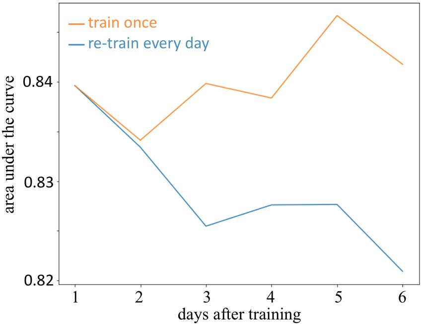
drops as we keep increasing the size of the window further. We attribute this observation10 Dmytro Karamshuk and David Matthews Fig. 7: The impact of the selected training window on the prediction performance of the model. to the highly volatile nature of the flight fares and use a training window of 7 days to train the model in production. Fig. 8: Model staleness of the one-off trained model vs. the model retrained every day. Model staleness To decide how frequently to retrain the model in production we mea- sure its staleness in an experiment (Fig. 8). We consider a six day long period with two variants: when the model is trained once before the start of the experiment and when the model is retrained every single day. The results suggest, that the one-off trained model quickly stales by an average of 0.3% in AUC with every day of the experiment. The model retrained every single day, although also affected by daily fluctuations, outper-
Learning Cheap and Novel Flight Itineraries   11

forms the one-off trained model. This result motivates our decision to retrain the model
every day.

                                                        dropped             added
                 share of total rules, %
                                           13
                                           12
                                           11
                                           10
                                                0   1     2     3     4   5             6
                                                        day of experiment

Fig. 9: Model stability, daily changes of (origin, destination, airline) rules inferred from
the random forest model.

Model stability Frequent retraining of the model comes at a price of its stability, i.e.,
giving the same prediction for the same input day in day out. To explain this phenom-
ena we look at the changes in the rules that the model is learning in different daily
runs. We generate a simplified approximation of our random forest model by pro-
ducing a set of decision rules of a form (origin, destination, airline), representing
the cases when combination itineraries with a given airline perform well on a given
(origin, destination) route. We analyse how many of the rules generated in day Ti−1
were dropped in the day Ti ’s run of the model and how many new ones were added
instead (Fig. 9).
    We see that around 88% of rules remain relevant between the two consecutive days
the remaining ≈ 12% are dropped and a similar number of new ones are added. Our
qualitative investigation followed from this experiment suggested that dropping a large
number of rules may end up in a negative user experience. Someone who saw a com-
bination option on day Ti−1 might be frustrated from not seeing it on Ti even if the
price went up and it is no longer in the top ten of the search results. To account for this
phenomenon we have introduced a simple heuristic in production which ensures that all
of the rules which were generated on day Ti−1 will be included for another day Ti .

4.2   Architecture of the pipeline
Equipped with the observations from the previous section we implement a machine
learning pipeline summarised in Fig. 10. There are three main components in the design
of the pipeline: the data collection process which samples the ground truth space to
12 Dmytro Karamshuk and David Matthews
generate training data; the training component which runs daily to train and validate the
model and the serving component which delivers predictions to the Skyscanner search
engine.
Serving Component
5% 90%
Skyscanner
Data Collection Current Model
Traffic
Apache Kafka Update Model
5%
Report Failure Passed?
Experiments with
Data Archive Challenger Model
AWS S3
Validation Data
Model Validation
5% of the last day
Data Querying
Pre-processing
AWS Athena
Training Data Model Training
7 recent days scikit-learn
Training Component (AWS CF + AWS Data Pipeline)
Fig. 10: The architecture of the machine learning pipeline.
Training infrastructure: The training infrastructure is orchestrated by AWS Cloud For-
mation6 and AWS Data Pipeline7 . The data querying and preprocessing is implemented
with Presto distributed computing framework8 managed by AWS Athena9 . The model
training is done with scikit-learn library on a high-capacity virtual machine. Our deci-
sion for opting towards a single large virtual machine vs. a multitude of small distributed
ones has been dictated by the following considerations:
Data volume: Once the heavy-lifting of data collection and preprocessing is done in
Presto, the size of the resulting training data set becomes small enough to be processed
on a single high capacity virtual machine.
Performance: By avoiding expensive IO operations characteristic of distributed
frameworks, we decreased the duration of a model training cycle to less than 10 min-
utes.
Technological risks: The proposed production environment closely resembles our
offline experimentation framework, considerably reducing the risk of a performance
difference between the model developed during offline experimentation and the model
run in production.
6
https://aws.amazon.com/cloudformation/
7
https://aws.amazon.com/datapipeline/
8
https://prestodb.io/
9
https://aws.amazon.com/athena/Learning Cheap and Novel Flight Itineraries 13
Traffic allocation We use 5% of Skyscanner search traffic to enable ground truth sam-
pling and prepare the data set for training using Skyscanner’s logging infrastructure10
which is built on top of Apache Kafka11 . We enable construction of all possible com-
bination itineraries on this selected search traffic, collecting a representative sample of
competitive and non-competitive cases to train the model. We use another 5% of the
search traffic to run a challenger experiment when a potentially better performing candi-
date model is developed using offline analysis. The remaining 90% of the search traffic
are allocated to serve the currently best performing model.
Validation mechanism We use the most recent seven days, Ti−7 ..Ti−1 , of the ground
truth data to train our model on day Ti as explained in section 4.1. We also conduct
a set of validation tests on the newly trained model before releasing it to the serving
infrastructure. We use a small share of the ground truth data (5% out of 5% of the
sampled ground truth data) from the most recent day Ti−1 in the ground truth data set
with the aim of having our validation data as close in time to when the model appears
in production on day Ti . This sampled validation set is excluded from the training data.
46
44
Recall@10
offline
42 production
40
38
0 1 2 3 4 5 6
day of experiment
Fig. 11: Performance of the model in offline experiments vs. production expressed in
terms of Recall@10 at 5% of quote requests.
4.3 Performance in production
When serving the model in production we allow a budget of an additional 5% of
quote requests with which we expect to reconstruct 45% of all competitive combination
itineraries (recall Fig. 6). From Fig. 11 we note that the recall measured in production
10
More details here https://www.youtube.com/watch?v=8z59a2KWRIQ
11
https://kafka.apache.org/14 Dmytro Karamshuk and David Matthews
deviates by ≈ 5% from expectations in our offline experiments. We attribute this to
model staleness incurred from 24 hour lag in the training data we use from the time
when the model is pushed to serve users’ searches.
Analysing the model’s impact on Skyscanner users, we note that new cheap combi-
nation itineraries become available in 22% of search results. We see evidence of users
finding these additional itineraries useful with a 20% relative increase in the booking
transactions for combinations.
5 Related work
Mining flights data The problem of airline fare prediction is discussed in detail in [2]
and several data mining models were benchmarked in [5]. The authors of [1] modelled
3D trajectories of flights based on various weather and air traffic conditions. The prob-
lem of itinerary relevance ranking in one of the largest Global Distributed Systems was
presented in [14]. The systematic patterns of airline delays were analysed in [7]. And
the impact of airport network structure on the spread of global pandemics was weighed
up in [4].
Location representation Traditional ways to model airline prices have been based on
complex networks [7][4] or various supervised machine learning models [5][14]. A
more recent trend is around incorporating neural embeddings to model location data.
Embeddings have seen great success in natural language processing [13], modelling
large graphs [16] and there has been a spike of enthusiasm around applying neural
embedding to geographic location context with a variety of papers focusing on: a) min-
ing embeddings from sequences of locations [15][20][12][20]; b) modelling geographic
context [19][6][9] and c) using alternative neural architectures where location represen-
tations are learned while optimising towards particular applications [19] and different
approaches are mixed together in [9] and [6]. The practicalities of augmenting existing
non-deep machine learning pipelines with neural embeddings are discussed in [21] and
in [3].
Productionising machine learning systems The research community has recently started
recognising the importance of sharing experience and learning in the way machine
learning and data mining systems are implemented in production systems. In [17] the
authors stress the importance of investing considerable thinking and resources in build-
ing long-lasting technological infrastructures for machine learning systems. The authors
of [10] describe their experiences in building a recommendation engine, providing a
great summary of business and technological constraints in which machine learning
researchers and engineers operate when working on production systems. In [18] the de-
velopers of Google Drive share their experience on the importance of reconsidering UI
metrics and launch strategies for online experimentation with new machine learning fea-
tures. Alibaba research in [11] emphasises the importance of considering performance
constraints and user experience and feedback in addition to accuracy when deploying
machine learning in production.Learning Cheap and Novel Flight Itineraries 15
6 Conclusions
We have presented a system that learns to build cheap and novel round trip flight
itineraries by combining legs from different airlines. We collected a sample of all such
combinations and found that the majority of competitive combinations were concen-
trated around a minority of airlines but equally spread across routes of differing pop-
ularity. We also found that the performance of these combinations in search results
increases as the time between search and departure date decreases.
We formulated the problem of predicting competitive itinerary combinations as a
trade-off between the coverage in the search results and the cost associated with per-
forming the requests to airlines for the quotes needed for their construction. We con-
sidered a variety of supervised learning approaches to model the proposed prediction
problem and showed that richer representations of location data improved performance.
We put forward a number of practical considerations for putting the proposed model
into production. We showed the importance of considering the trade-off between the
model stability and staleness, balancing keeping the model performant whilst minimis-
ing the potential negative impact on the user experience that comes with changeable
website behaviour.
We also identify various considerations we took to deliver proposed model to users
including technological risks, computational complexity and costs. Finally, we provided
an analysis of the model’s performance in production and discuss its positive impact on
Skyscanner’s users.
Acknowledgement
The authors would like to thank the rest of the Magpie team (Boris Mitrovic, Calum
Leslie, James Eastwood, Linda Edstrand, Ronan Le Nagard, Steve Morley, Stewart
McIntyre and Vitaly Khamidullin) for their help and support with this project and the
following people for feedback on drafts of this paper: Bryan Dove, Craig McIntyre,
Kieran McHugh, Lisa Imlach, Ruth Garcia, Sri Sri Perangur, Stuart Thomson and Tatia
Engelmore.
References
1. Ayhan, S., Samet, H.: Aircraft trajectory prediction made easy with predictive analytics. In:
KDD. pp. 21–30 (2016)
2. Boyd, E.: The future of pricing: How airline ticket pricing has inspired a revolution. Springer
(2016)
3. Chamberlain, B.P., Cardoso, A., Liu, C.H., Pagliari, R., Deisenroth, M.P.: Customer life time
value prediction using embeddings. In: Proceedings of the ninth ACM SIGKDD international
conference on Knowledge discovery and data mining. ACM (2017)
4. Colizza, V., Barrat, A., Barthélemy, M., Vespignani, A.: The role of the airline transportation
network in the prediction and predictability of global epidemics. Proceedings of the National
Academy of Sciences of the United States of America 103(7), 2015–2020 (2006)16 Dmytro Karamshuk and David Matthews
5. Etzioni, O., Tuchinda, R., Knoblock, C.A., Yates, A.: To buy or not to buy: mining airfare
data to minimize ticket purchase price. In: Proceedings of the ninth ACM SIGKDD interna-
tional conference on Knowledge discovery and data mining. pp. 119–128. ACM (2003)
6. Feng, S., Cong, G., An, B., Chee, Y.M.: Poi2vec: Geographical latent representation for
predicting future visitors. In: AAAI. pp. 102–108 (2017)
7. Fleurquin, P., Ramasco, J.J., Eguiluz, V.M.: Systemic delay propagation in the us airport
network. Scientific reports 3, 1159 (2013)
8. Guo, C., Berkhahn, F.: Entity embeddings of categorical variables. arXiv preprint
arXiv:1604.06737 (2016)
9. Kejriwal, M., Szekely, P.: Neural embeddings for populated geonames locations. In: Interna-
tional Semantic Web Conference. pp. 139–146. Springer (2017)
10. Liu, D.C., Rogers, S., Shiau, R., Kislyuk, D., Ma, K.C., Zhong, Z., Liu, J., Jing, Y.: Related
pins at pinterest: The evolution of a real-world recommender system. In: Proceedings of the
26th International Conference on World Wide Web Companion. pp. 583–592. International
World Wide Web Conferences Steering Committee (2017)
11. Liu, S., Xiao, F., Ou, W., Si, L.: Cascade ranking for operational e-commerce search. In:
Proceedings of the 23rd ACM SIGKDD International Conference on Knowledge Discovery
and Data Mining. pp. 1557–1565. ACM (2017)
12. Liu, X., Liu, Y., Li, X.: Exploring the context of locations for personalized location recom-
mendations. In: IJCAI. pp. 1188–1194 (2016)
13. Mikolov, T., Sutskever, I., Chen, K., Corrado, G.S., Dean, J.: Distributed representations of
words and phrases and their compositionality. In: Advances in neural information processing
systems. pp. 3111–3119 (2013)
14. Mottini, A., Acuna-Agost, R.: Deep choice model using pointer networks for airline itinerary
prediction. In: Proceedings of the 23rd ACM SIGKDD International Conference on Knowl-
edge Discovery and Data Mining. pp. 1575–1583. ACM (2017)
15. Pang, J., Zhang, Y.: Deepcity: A feature learning framework for mining location check-ins.
arXiv preprint arXiv:1610.03676 (2016)
16. Perozzi, B., Al-Rfou, R., Skiena, S.: Deepwalk: Online learning of social representations. In:
Proceedings of the 20th ACM SIGKDD international conference on Knowledge discovery
and data mining. pp. 701–710. ACM (2014)
17. Sculley, D., Holt, G., Golovin, D., Davydov, E., Phillips, T., Ebner, D., Chaudhary, V., Young,
M., Crespo, J.F., Dennison, D.: Hidden technical debt in machine learning systems. In: Ad-
vances in Neural Information Processing Systems. pp. 2503–2511 (2015)
18. Tata, S., Popescul, A., Najork, M., Colagrosso, M., Gibbons, J., Green, A., Mah, A., Smith,
M., Garg, D., Meyer, C., et al.: Quick access: Building a smart experience for google drive.
In: Proceedings of the 23rd ACM SIGKDD International Conference on Knowledge Discov-
ery and Data Mining. pp. 1643–1651. ACM (2017)
19. Yan, B., Janowicz, K., Mai, G., Gao, S.: From itdl to place2vec–reasoning about place type
similarity and relatedness by learning embeddings from augmented spatial contexts. Pro-
ceedings of SIGSPATIAL 17, 7–10 (2017)
20. Zhao, S., Zhao, T., King, I., Lyu, M.R.: Geo-teaser: Geo-temporal sequential embedding rank
for point-of-interest recommendation. In: Proceedings of the 26th International Conference
on World Wide Web Companion. pp. 153–162. International World Wide Web Conferences
Steering Committee (2017)
21. Zhu, J., Shan, Y., Mao, J., Yu, D., Rahmanian, H., Zhang, Y.: Deep embedding forest: Forest-
based serving with deep embedding features. In: Proceedings of the 23rd ACM SIGKDD
International Conference on Knowledge Discovery and Data Mining. pp. 1703–1711. ACM
(2017)You can also read