PROCESSING LIDAR DATA FROM A VIRTUAL LOGISTICS SPACE - DROPS
←
→
Page content transcription
If your browser does not render page correctly, please read the page content below
Processing LiDAR Data from a Virtual Logistics
Space
Jaakko Harjuhahto
Aalto University, Department of Computer Science, Espoo, Finland
jaakko.harjuhahto@aalto.fi

Anton Debner
Aalto University, Department of Computer Science, Espoo, Finland
anton.debner@aalto.fi

Vesa Hirvisalo
Aalto University, Department of Computer Science, Espoo, Finland
vesa.hirvisalo@aalto.fi

      Abstract
We study computing solutions that can be used close to the network edge in I2oT systems (Industrial
Internet of Things). As a specific use case, we consider a factory warehouse with AGVs (Automated
Guided Vehicles). The computing services for such systems should be dependable, yield high
performance, and have low latency. For understanding such systems, we have constructed a hybrid
system that consists of a simulator yielding virtual LiDAR sensor data streams in real-time and a
sensor data processor on a real cluster that acts as a fog computing node close to the warehouse.
The processing merges the observations done from the individual sensor streams without using the
vehicle-to-vehicle communication links for the complicated computing. We present our experimental
results, which show the feasibility of the computing solution.

2012 ACM Subject Classification Computer systems organization → Embedded and cyber-physical
systems; Computing methodologies → Modeling and simulation; Computing methodologies →
Distributed computing methodologies

Keywords and phrases simulation, hybrid systems, new control applications, fog computing

Digital Object Identifier 10.4230/OASIcs.Fog-IoT.2020.4

Funding This work has been financially supported by the Technology Industries of Finland Centennial
Foundation.

Acknowledgements We would like to thank research assistant Matias Hyyppä for his work on the
dataset creation tools and the anonymous reviewers of this paper for their valuable comments.

 1      Introduction
In this paper, we address the computing structures that are needed in intelligent traffic
systems for warehouse logistics and in the related research and development work. The
traditional systems rely on central controllers that coordinate the motion of the vehicles.
Recent developments in AI (Artificial Intelligence) are enabling many new approaches
including autonomous driving that relies heavily on rich sensor data collected on the traffic
situations.
    The systems need to process large amounts of sensor data in real-time to maintain an
understanding of the ever-changing traffic situation. The computing services for such systems
should be dependable, yield high performance, and have low latency. The traditional terminal
computing devices (e.g., on the vehicles) or cloud computing services based large data centers
are not sufficient. Fog computing solutions are one option to enable such applications (see
[10] and [20] for related approaches).
            © Jaakko Harjuhahto, Anton Debner, and Vesa Hirvisalo;
            licensed under Creative Commons License CC-BY
2nd Workshop on Fog Computing and the IoT (Fog-IoT 2020).
Editors: Anton Cervin and Yang Yang; Article No. 4; pp. 4:1–4:12
                    OpenAccess Series in Informatics
                    Schloss Dagstuhl – Leibniz-Zentrum für Informatik, Dagstuhl Publishing, Germany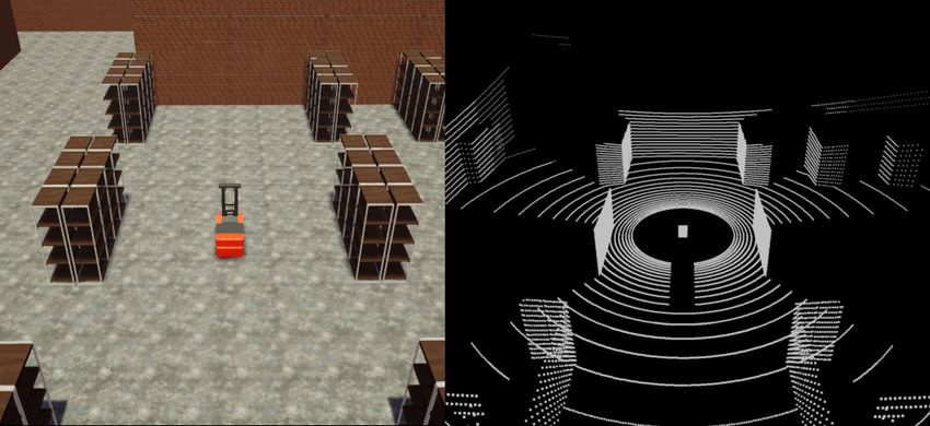
4:2   Processing LiDAR Data from a Virtual Logistics Space

          The fog computing paradigm addresses the ways of acting between devices and centralized
      cloud services, utilizing resources in between them, and thus allowing sufficient resources
      close to the devices. Even though some standards exist (e.g., [7]), many aspects of the
      problem of communicating and managing resources on the Cloud to Things continuum need
      more research. There has been several proposals and studies on the clusters (also mini data
      centers, cloudlets, etc.) needed in fog computing solutions [22].
          Warehouse AGVs are rather typical mobile robots. Their operation is complex including
      localization, motion planning, and control. Traditionally their warehouse environment is
      augmented to ease their operation (by using markers, reflectors, etc.). As flexibility is
      essential and human presence is often needed, the technology is developing toward natural
      navigation. Such navigation solutions are often based on sensors perceiving the environment,
      and the development of such systems typically calls for suitable simulators [4].
          Our study addresses LiDAR (laser scanner) data processing for AGV coordination. For
      efficient coordination of the flow of the traffic inside a warehouse, the LiDAR data of the
      participating vehicles is needed. Using the shared data, vehicles can also help each other to
      see around corners, and thus, avoid being over-cautious, when there is human presence in a
      warehouse. However, constructing a shared real-time view calls for plenty of communication.
      Using, e.g., V2V (Vehicle-to-Vehicle) links for computing the shared view can cause massive
      use of the wireless communication links.
          Our contribution consists of three parts. Firstly, we have built a hybrid setup for research
      and development purposes. Our hybrid setup uses a virtual warehouse with virtual AGVs
      and a real cluster for their data processing. Secondly, we have implemented LiDAR data
      processing that is suitable for control algorithms and does the computing of the shared
      view within the cluster. Our approach supports both scalability and fault-tolerance of the
      processing. Thirdly, we present performance measurements that show the feasibility of
      our approach.
          The structure of this paper is as follows. We begin by reviewing AGV systems for
      warehouse logistics and describing our warehouse case with the simulation model that
      we have made in Section 2. We continue by explaining the designed computation and
      communication architecture in Section 3. We describe our hybrid simulation setup and our
      LiDAR data processing in Section 4. We present our experimentation with the setup in
      Section 5, and discuss our results in Section 6. We end the presentation with our conclusions.

       2     AGVs in a Factory Warehouse
      We have made a model of a warehouse hall. Our modeling is motivated by the modern factory
      warehouses. In this section, we first review modern factory warehouses in Subsection 2.1,
      and then, describe our modeling in Subsection 2.2.

      2.1    Modern Factory Warehouses
      The operation of manufacturing plants depend on logistics. Manufacturing plants typically
      have warehouse spaces, through which the goods needed in production flow. The operation
      of warehouses calls for careful optimization as everything needed should be available, but
      storing excessive amounts of goods should be avoided as the storage costs are usually high. In
      addition to speed, flexibility is essential as factories typically have to adjust their operation
      frequently.
          Warehouse operation in factories is still mostly manual, but automation is entering the
      scene. Warehousing in factories of the future can rely on AGVs and integrated systems
      for logistics. AGVs typically move goods between locations in a plant environment and
J. Harjuhahto, A. Debner, and V. Hirvisalo 4:3
CARLA simulator Realtime simulation Offline (realtime) replay
Warehouse
AGVs Sensor Sensor
data stream Java data stream Data processing
Humans Python client
HDF5-file replay client cluster
TCP TCP
LiDARs
Figure 1 Overview of our setup. CARLA is first used to run our warehouse simulation and
produce sensor data streams in real-time. These streams are captured with a Python client and
stored in a hierarchical data format (HDF5). The HDF5 files can then be used to replay the real-time
sensor data streams without running the CARLA simulator. The advantage of this approach is full
reproducibility and control over sending data to our data processing cluster.
the warehouse is central for them. The AGV system is usually controlled by a centralized
Warehouse Management System (WMS). Both the navigation of the AGVs in flexible
warehouse environments and their co-operation with humans call for advanced sensing
technology.
Sabattini et al. [19] give a view on advanced sensing technology for AGV systems and the
related warehouse operations. Currently, LiDARs are the typical main sensor for AGVs as
they directly yield distance data. However, obstacles limit the view of LiDARs, and limited
understanding of a traffic situation can cause unnecessary slow-downs or complete stops for
the AGVs. This underlines the need for shared sensing and sensor fusion.
In mobile robotics, understanding of traffic situations is often done by using two-
dimensional occupancy grids [4]. An occupancy grid is an abstract representation of the
physical situation, where each grid cell indicates the state of the corresponding physical place.
Occupancy grids can be used together with robot control algorithms (see, e.g., [14]). The
predictions of movements are important for such algorithms, and the history of observations is
useful for such predictions [15]. The coordination of multiple robots in intersections presents
an important and challenging optimization problem, for which DMPC (Distributed Model
Predictive Control) methods are promising [11]. Our design of data processing has been
impacted by the needs of such algorithms.
2.2 A Model for a Warehouse
Our goal was to create a simple, easily modifiable virtual warehouse. This was achieved by
creating a grid-based structure from modular squares and storage shelf units. Each square
is 5 x 5 m2 in size, leaving a moderately large working space between the storage shelves.
A portion of the resulting warehouse is shown in Figure 2. The modular nature of the
warehouse enabled us to experiment with various sizes, for example, varying the storage area
from 20 x 20 m2 to 50 x 50 m2 . As the AGVs sense their surroundings only through LiDARs,
the graphical details of the warehouse are not important. While the shelf-models appear to
be empty in Figure 2, we simplify the scenario by assuming that they are fully populated by
stored objects and therefore preventing LiDARs from seeing through the shelves at all.
3 Computing and Communication Architecture
We consider an AGV system that uses LiDAR sensing for shared environment perception.
As walls limit the sensing, the halls of the whole plant form distinct physical areas, where
shared sensing is the most useful. Thus, in our design we concentrate on sensing inside a
Fo g - I o T 2 0 2 04:4 Processing LiDAR Data from a Virtual Logistics Space
single hall and assume that the processing of the LiDAR data from the hall is done by a
single fog node (i.e., a computing cluster). A large plant can have multiple fog nodes, each
serving one or more distinct areas.
Our architecture design is inspired by the work of Farkas et al. [5] in many ways. They
describe a rather generic approach for using 5G-TSN systems (5G integrated Time-Sensitive
Networking) for industrial applications. The integration of 5G and TSN is rather complex,
but there exists extensive documentation for both 5G systems and TSN systems (see, e.g.,
[17] for further information). However, from the communication perspective of an application
much of the complexity of a 5G system can be abstracted by a TSN system on top of it.
The architecture as such does not limit the number of the AGVs connected to a fog
node or the number of compute nodes inside the cluster. However, the computation and
communication capacity of a fog node limit these numbers in practice.
Figure 3 describes our design. The AGVs are connected to the fog node using TSN
connections over a wireless 5G network. The whole system runs under central control
(SDN controller), which includes the related CUC (Centralized User Configuration) and
CNC (Centralized Network Configuration) elements. The controller coordinates both the
distributed mini-datacenter (i.e., the fog nodes) and the integrated 5G-TSN system. We
assume the cluster intra-connections to be much faster than the wireless connections through
separate interfacing (IF) toward the AGVs.
The connection in TSN system exists between the TSN end stations (ES). The connections
appear as TSN bridges that are virtualized on top of the underlying 5G system. The 5G
system has TSN translation (TT) functionality for mapping the user and control planes
towards TSN. This mapping is essential in hiding the 5G details from the TSN connections.
In our current design, we use only single PDU (Protocol Data Unit) sessions between the end
points. Inside the 5G system, User Plane Functions (UPF) connect to the AGVs through
the links between the base stations (gNB). From the 5G system viewpoint, the AGVs appear
as UEs (User Equipment). In our current design, we have only one UE within an AGV.
4 Hybrid Processing Setup
Our hybrid setup is based on the CARLA simulator [3] producing virtual sensor data streams
and a real cluster processing these data streams. The setup is illustrated in Figure 1. The
sensor streams produced by the simulator are stored in a dataset file. The details of the
simulation and virtual data streams are described in Subsection 4.1.
Figure 2 Virtual model of a warehouse, where workers can walk freely among autonomous
vehicles.J. Harjuhahto, A. Debner, and V. Hirvisalo 4:5
5G system
SDN
Control elements Controller
tion
Control plane
era
Fed
User plane
AGV ES TSN Bridge Compute
TT UE gNB UPF TT ES IF
device
..
virtual bridge
elements Node
..
Switch
TSN Bridge Compute
AGV ES TT UE gNB UPF TT ES IF
elements Node
device virtual bridge
Fog node (cluster)
Figure 3 The designed architecture for a single fog node and its connections in the system. The
fog nodes can be federated under a single SDN (Software Defined Networking) controller. The AGV
devices (left) implement both the TSN (Time Sensitive Networking) end stations and act as 5G
system UEs. The fog node (right) communicates with the AGVs by using TSN connections over the
wireless 5G network.
The sensor data streams are replayed from the stored dataset file in real-time and processed
by the cluster. In our setup, the replay clients simulate the 5G-TSN communication. The
modeling and simulation of the 5G-TSN communication is described in Subsection 4.2.
The processing cluster implements state sharing by distributing the observations computed
from the LiDAR data streams. The details of the processing cluster and the related experiment
are described in Subsection 4.3.
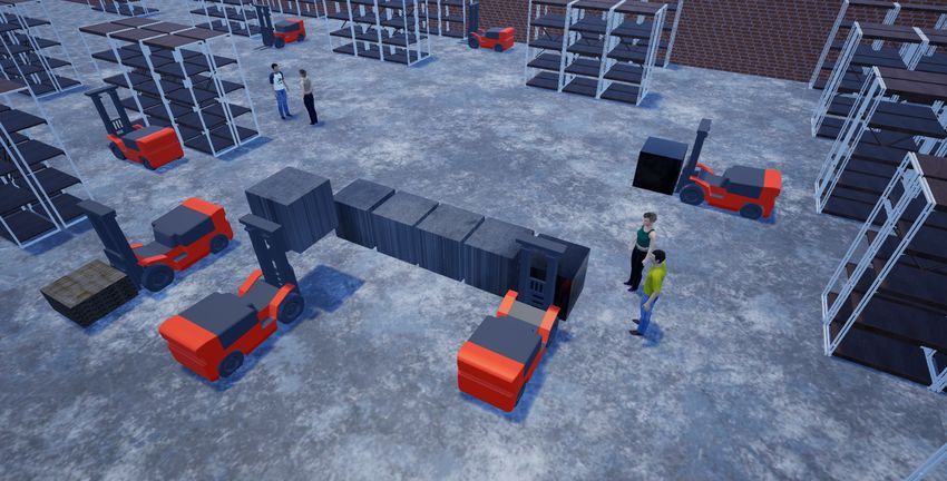
4.1 Generation of Virtual Sensor Data
Figure 4 An example of the data produced by CARLA with a LiDAR sensor attached to an
AGV. Left: RGB view of the simulation scene. Right: 3D view of the LiDAR data.
As shown on the left side of Figure 1, we used CARLA to simulate AGVs and humans
moving together inside a warehouse. CARLA [3] is an open-source simulator made for
autonomous driving research. Its main features include modern rendering pipeline, animated
pedestrians, fully controllable vehicles, pre-made urban cities and various simulated sensors,
such as cameras and LiDARs. Python clients can be used to control the simulation actors
and process sensor data remotely over TCP.
Fo g - I o T 2 0 2 04:6 Processing LiDAR Data from a Virtual Logistics Space
Implementation
Simulator on real hardware
5G-TSN network Scheduler
Compute
Warehouse
node
..
ES simulated bridge ES
..
Switch
Queue
.. ..
Egress
Ingress
Mux
. Compute . .
ES simulated bridge ES
node Queue
Figure 5 On the left side, the simulation of the 5G-TSN system within the hybrid set-up is
shown. The replay client acts as a simulator that communicates with the cluster. On the right side,
details of the TSN connection simulation are shown.
We created a Python client for collecting data from the simulation and storing it in to a
dataset with hierarchical data format (HDF5 [21]). The dataset used in our experiment is
available at [2]. For the work described in this paper, the relevant stored data are LiDAR
point clouds, simulation actor positions and rotations for every time step. Velocities of the
actors and data from all other kinds of sensors can also be included in a dataset on demand,
enabling further development branches for more advanced logistic experiments.
CARLA produces the LiDAR data by performing raycasts from the rotating LiDAR
sensor on each simulation step. Each raycast returns the point of first collision with any
other object along the ray. The resulting data is essentially a set of coordinates in a 3D
space, where the origo is the sensor itself. An example of this data is visualized in Figure 4.
While the LiDAR sensor attempts to imitate its real-life counterparts, it is not completely
realistic in the sense that the measurement are absolute ground truths without any noise or
reflections. Such artefacts can be added to simulate realistic conditions.
4.2 Real-time Simulation
The stored datasets represent situations, where AGVs move and perceive their environment.
As illustrated in Figure 1, these situations are replayed from HDF5 files in real-time. From
the view point of the application, this is identical to a situation, where the CARLA simulator
would be directly connected to the fog system.
The fog system is modeled within the replay client, which acts as a real-time simulator.
The setup is illustrated in Figure 5. The communication between warehouse simulator (i.e.,
a replay based on a CARLA data set) and the fog cluster consists of real data items, but
their motion in the larger communication system is simulated. Real data transmissions
happen between the fog simulator and the computing cluster as the computing cluster is not
virtual but consists of real pieces of hardware. Also, the data transmission within the cluster
are real.
In the simulation of the fog system, we do not simulate the underlying 5G system in detail.
Instead of the detailed simulation, we simulate the TSN bridges on top of the 5G system. In
our setup, their main function is the wireless communication within the AGV system.
Simulating the operation of the TSN connections is illustrated in the Figure 5 (right side).
There can be multiple streams that go over a TSN connection, but we do not model any
hierarchy between the streams. Further, there is no modeling of any complex underlyingJ. Harjuhahto, A. Debner, and V. Hirvisalo 4:7
functions (e.g., traffic shaping). The entering streams (Ingress) are buffered into queues that
are scheduled into a time division multiplexer (Mux) before being sent (Egress). Thus, the
simulation model is rather abstract compared to a real TSN system on top of a 5G network,
but it allows for the testing of various real-time scheduling algorithms together with realistic
delay models of the processing and communication steps.
4.3 Intelligent Traffic Coordination with a Cluster
We use a cluster of small compute nodes to maintain the state of the occupancy grid
and process LiDAR point clouds from AGVs. The server software is written in C++ and
communicates with AGVs and peer nodes with TCP sockets. Data is serialized using
FlatBuffers [6]. Every node runs the same software and maintains a copy of the occupancy
grid state to provide redundancy and availability. In case of node failures, AGVs using the
cluster may simply switch to another node.
Each cluster node can receive data from AGVs. Once a node receives a LiDAR point
cloud, it will check if it has local capacity to process the data frame. If a local worker thread
has signaled that it is ready to pull work, the frame is dispatched to that worker. If no local
worker capacity is available, the data frame is forwarded to the peer node with the most
capacity available at the moment. Each node reports on its available worker capacity to the
rest of the cluster. Figure 6 shows the related communication patterns. Once the cluster has
accepted a LiDAR data frame from an AGV, it guarantees processing of that frame, barring
hardware failure.
Sensor stream
Node #1
Workload sharing
Worker threads Node #2 Node #3
Observation sharing
Figure 6 Processing cluster. The cluster consists of computation nodes, that can share their
workload and observations between each other. Each node has a pool of worker threads. The number
and capabilities of these threads depend on the node’s hardware resources. Each node is capable of
receiving sensor (LiDAR) data from the AGVs. While the ability to share resources enable flexible
setups, in this image each node is receiving a sensor stream from a single AGV.
Processing a set of LiDAR data points is a two-phase process, as shown in Figure 7.
During the first step, we compute which cells the LiDAR rays either hit or pass through
adapting Bresenham’s line algorithm [1] to our occupancy grid. We consider LiDAR ray
hits as having priority. If LiDAR rays have both hit something in a cell and passed through
the cell, we consider the cell occupied. These observations on the states of a subset of all
cells in the occupancy grid are collected and published to every peer node in the cluster.
During the second step, replicated on each node, the observations are committed to the grid
data structure. Finally, the node that received the LiDAR data from an AGV will calculate
the heuristic cell state and return the entire grid to the AGV. This updated occupancy grid
also includes all the observations from other AGVs applied to the compute nodes grid. The
Fo g - I o T 2 0 2 04:8 Processing LiDAR Data from a Virtual Logistics Space
occupancy grid supports concurrent updates from multiple LiDAR frames by implementing
concurrency controls on the level of individual cells. If multiple updates overlap, all the
observations are recorded to be used as inputs for determining the cell’s current state later on.
~10 000 ~100
measurements observations
LiDAR Compute
Update grid
point cloud observations
Figure 7 Simplified process view. In our case, each set of LiDAR measurements consists of
a point cloud with over 10 000 points in a 3D coordinate system. These measurements are then
squeezed into a far fewer number of observations. Each observation determines the state of a single
cell in the grid at that point in time. These observations are then combined with the previous
information of the grid, in order to form an updated understanding of the environment.
Our model of an occupancy grid is static and regular. Using a static grid of predetermined
resolution allows all of the compute nodes to use the same coordinates for occupancy grid
cells without necessitating a fully consistent state coherency protocol stemming from the
use of dynamic grids. For each cell in the grid, we store the timestamp of the most recent
observations of each state we track: ’free’, ’occupied’ and ’vehicle’. Cells that have never
been observed are considered as ’unknown’. The category ’vehicle’ cells are derived directly
from the positions reported by of each of the AGVs. We apply an exponential decay term
(P (t) = e−γt ) to model diminishing trust in the cell’s state as time progresses, unless new
observations are made, refreshing the timestamps. Suitably chosen constants γ for each state
category allows the AGVs using the occupancy grid for guidance decisions to consider the
reliability of the knowledge on the current state of individual cells. Cells never explicitly
revert back to an ’unknown’ state, but AGVs should consider cells with a low reliability as
effectively unknown. Figure 8 presents an example of a small occupancy grid.
Free
Unknown
Occupied
Vehicle
Figure 8 Distributed occupancy grid. Multiple AGVs collaborate to create a shared understanding
of the surrounding environment. The grid is divided into cells, that represent the latest observations
made from the AGV sensor data.
5 Experimental Results
We validated our design by performing an experiment by using pre-recorded sensor data as
described in Section 4.1 to stream LiDAR point clouds to the cluster. The cluster hardware
is Intel Atom x5-8350 based commodity-off-the-shelf (COTS) computers connected to a
router. The cluster consists of seven compute nodes, all running Ubuntu 18.04 LTS. An
additional workstation computer was used to read the sensor data from HDF5 files and push
data frames to the cluster at regular 100 ms intervals. We used a warehouse model of 50
meters by 50 meters and an occupancy grid of 1 m by 1 m cells.J. Harjuhahto, A. Debner, and V. Hirvisalo 4:9
Shared Ingress Node Dedicated Ingress Node per AGV
1 1
0.9 0.9
0.8 0.8
Cumulative distribution function
Cumulative distribution function
0.7 0.7
0.6 0.6
0.5 0.5
0.4 0.4
0.3 0.3
0.2 0.2
2 AGVs 2 AGVs
0.1 4 AGVs 0.1 4 AGVs
6 AGVs 6 AGVs
0 0
40 50 60 70 80 90 100 40 50 60 70 80 90 100
Latency [ms] Latency [ms]
Figure 9 Cumulative distribution of end-to-end latencies in milliseconds. On the left, a single
compute node acts as the ingress point for all of the LiDAR data produced by AGVs. On the right,
each AGV connects to a distinct compute node.
Average total latency
Process LiDAR frame
Compute grid update
Communication
Store observations
0 10 20 30 40 50 60 70
Milliseconds
Figure 10 Breakdown of how the individual steps in the end-to-end process, described above,
contribute to the observed average total latency. The values are from averaging the results over all
of the tests.
The simulation consists of one human walking across the entire warehouse, while 2 to 6
robots follow their own predetermined paths between the storage shelves. The data is
collected over a 30 second simulation at 10 samples per second, which matches the 100 ms
replay interval. The LiDARs are rotating around their axis at 10 Hz, which means that each
LiDAR sensor produces a full 360 degree scan of the environment during each sample. Each
LiDAR produced 2500 data points per frame, or 25000 points per second. The dataset is
designed to start and stop in roughly the same state configuration to support looped replay.
In the experiment, we measure the end-to-end latency from the point where LiDAR
data frame passes through the simulated 5G bridge to the cluster to the point in time
when the cluster has returned a new version of the entire occupancy grid over the same
simulated 5G connection. Our simulated network offered 500 Mbit/s of upstream and
downstream bandwidth divided fairly across every active connection. We perform this
latency measurement for 2, 4 and 6 simultaneous AGVs using two strategies for transferring
data frames to and from the cluster. In the first arrangement, a single compute node in the
cluster acts as service endpoint for all of the AGVs, accepting LiDAR frames and routing
these to peer nodes for processing. In the second arrangement, every AGV connects directly
to a distinct compute node so that the nodes have sufficient local capacity to process the
LiDAR frame and share only the computed observations with the rest of the cluster. Data
is collected over 6k LiDAR frames per AGV. Figure 9 presents the cumulative distribution
functions of these latency measurements. Additional, Figure 10 presents a breakdown of the
relative contribution to the total latency by each of the phases in the end-to-end process.
We measured the CPU utilization of all the compute nodes in the cluster during the
experiment to understand how the system scales in terms of processing data volumes and
how the compute tasks are distributed within the cluster. The results of our utilization
Fo g - I o T 2 0 2 04:10 Processing LiDAR Data from a Virtual Logistics Space
Shared Ingress Node Dedicated Ingress Node per AGV
250 250
node1 node1
node2 node2
Cumulative Node CPU utilization [%] node3 node3
Cumulative Node CPU utilization [%]
200 node4 200 node4
node5 node5
node6 node6
node7 node7
150 150
100 100
50 50
0 0
2 4 6 2 4 6
Number of AGVs Number of AGVs
Figure 11 Cumulative CPU utilization of compute nodes in the cluster. On the left, a single
compute node acts as the ingress point for all of the LiDAR data produced by AGVs. The computer
“node1” acts as the shared ingress point. On the right, each AGV connects to a distinct compute
node.
measurements are presented in Figure 11. The results show that the total compute load is
equivalent for both ingress arrangements, but the compute balance across nodes varies. For
the shared ingress node arrangement, the node acting as the gateway is under significantly
more load than the rest of the cluster. For 6 AGVs, the shared ingress node is under sufficient
load to cause degradation of responsiveness, as is evident in the latency results of Figure 9.
As can be seen from the figures, incoming data streams can be added to the cluster
without significantly affecting the latency. The size of the warehouse is realistic, but even
with a cluster with modest computing power, we are able to get reasonable latencies (on
average 60 ms). It is important to notice that the latencies are about perceiving the overall
situation in the warehouse hall. The individual vehicles may need shorter perception latencies
for their internal control.
A more powerful cluster is needed for handling denser LiDAR streams and more vehicles,
but our solution uses the internal communication links of a cluster to update an occupancy
grid. Using, e.g., vehicle-to-vehicle links for the purpose would be inefficient and slow, as
would be using distant cloud computing capacity.
6 Discussion
Instead of handling LiDAR data locally in the AGVs, our design is based on sending the
LiDAR data to a fog node. Our main motivation is to enable the use of novel computing
intensive methods for shared perception. Recently, methods based on machine learning
have improved significantly and gained attention. Such methods are based on having the
raw data directly available for processing and massive computing capacity for applying the
computationally intensive algorithms (see [18] and [13] for related surveys). We see fog
computing as a good solution for such needs. On one hand, it enables the use of complex
software solutions on computationally powerful hardware. On the other hand, fog computing
nodes can be placed close to the AGVs, which makes short latency times possible.
We have chosen a solution based on 5G-TSN systems as they enable real-time operation
of the communication network. Other options for organizing the communication exist (see,
e.g., [22] for a survey). Such systems are currently under intense research and development
work, but not ready for wide scale experimentation. This has motivated us to use simulation
as the primary method for our studies. However, modeling and understanding the behaviorJ. Harjuhahto, A. Debner, and V. Hirvisalo 4:11
of the related complex software is hard. Software layers abstract the details, and there is
the risk that simulation models do not capture the complex dependencies hidden by the
abstraction layers. Therefore, we have used a hybrid approach, where such software parts
of the system are implemented by using real software running on real hardware. Using a
generic fog simulator, e.g. [9], would give a different view into AGV systems.
We have not used computational accelerators in our experimentation. Using computational
accelerators for handling LiDAR point data is common. It is also typical to use accelerators
in machine learning inference systems. Our intention has been to present an overview of
a perception system based on a fog node. Our own prior work [8] indicates that the use
of typical computational accelerators further complicates the operation of the systems. In
the experimentation presented in this paper, we have used small point clouds instead of
having computational accelerators, e.g. GPUs, in the system. Similarly, we have omitted the
detailed features and analysis of TSN operation as we have concentrated on the system level
properties (for detailed features and analysis of TSN operation see, e.g., [12, 16]).
7 Conclusions
In this paper, we presented our hybrid solution for doing research and development work
on intelligent AGV traffic systems. Our solution combines a virtual warehouse with a real
cluster acting as a fog computing node close to the warehouse. Our experimentation shows
that our implementation of the AGV LiDAR sensor data processing on the cluster is feasible
for producing a shared view of the observations done from the sensor data streams.
The occupancy information that we compute on a cluster yields a shared real-time view
of an observed situation. Our design is based on using hard real-time methods, but in the
experimentation we have used simplifications. We see more detailed analysis of the real-time
behavior is an important direction for future research.
By sharing the observations and keeping up history, our design supports fault-tolerance
and offers information on the motion of the parties in the warehouse. Motion information
is typically needed by the traffic control algorithms that coordinate several vehicles. Also
considering the fault-tolerance aspects, there is a need for further research.
To get results on traffic coordination, a shared control algorithm could be implemented
using the shared LiDAR observation data available in the cluster. Also, AI systems could
be added both to the vehicles and to the management system to understand the interplay
between the autonomy of vehicles and coordinated decisions by the traffic controller.
References
1 Jack E. Bresenham. Algorithm for computer control of a digital plotter. IBM Systems journal,
4(1):25–30, 1965. doi:10.1147/sj.41.0025.
2 Anton Debner, Jaakko Harjuhahto, and Vesa Hirvisalo. A LiDAR dataset from a virtual ware-
house. Aalto University, 2020. URL: https://github.com/Aalto-ESG/fog-iot-2020-data.
3 Alexey Dosovitskiy, German Ros, Felipe Codevilla, Antonio Lopez, and Vladlen Koltun.
CARLA: An open urban driving simulator. In Proceedings of the 1st Annual Conference on
Robot Learning, pages 1–16, 2017.
4 Gregory Dudek and Michael Jenkin. Computational principles of mobile robotics. Cambridge
University Press, 2010.
5 Janos Farkas, Balasz Varga, György Miklos, and Joachim Sachs. 5G-TSN Integration for
Industrial Automation. Ericsson Technology Review, 07/2019.
6 FlatBuffers. The FlatBuffers website, 2020. URL: https://google.github.io/flatbuffers/.
7 OpenFog Consortium Architecture Working Group. OpenFog reference architecture for fog
computing. OPFRA001, 20817:162, 2017.
Fo g - I o T 2 0 2 04:12 Processing LiDAR Data from a Virtual Logistics Space
8 Jussi Hanhirova, Teemu Kämäräinen, Sipi Sipilä, Matti Siekkinen, Vesa Hirvisalo, and Antti
Ylä-Jääski. Latency and throughput characterization of convolutional neural networks for
mobile computer vision. In Proceedings of the 9th ACM Multimedia Systems Conference
(MMSys’18), 2018. doi:10.1145/3204949.3204975.
9 iFogSim. A Toolkit for Modeling and Simulation of Resource Management Techniques in
Internet of Things, Edge and Fog Computing Environments. URL: https://github.com/
Cloudslab/iFogSim.
10 Vasileios Karagiannis. Compute node communication in the fog: Survey and research challenges.
In Proceedings of the Workshop on Fog Computing and the IoT, pages 36–40, 2019. doi:
10.1145/3313150.3313224.
11 Alexander Katriniok, Peter Kleibaum, and Martina Joševski. Distributed model predic-
tive control for intersection automation using a parallelized optimization approach. IFAC-
PapersOnLine, 50(1):5940–5946, 2017. doi:10.1016/j.ifacol.2017.08.1492.
12 Dorin Maxim and Ye-Qiong Song. Delay Analysis of AVB traffic in Time-Sensitive Networks
(TSN). In Proceedings Real-Time Networks and Systems (RTNS’17), 2017. doi:10.1145/
3139258.3139283.
13 Ruben Mayer and Hans-Arno Jacobsen. Scalable Deep Learning on Distributed Infrastructures:
Challenges, Techniques, and Tools. ACM Compututing Surveys, 53(1), February 2020. doi:
10.1145/3363554.
14 Mohamed W. Mehrez, Tobias Sprodowski, Karl Worthmann, George K.I. Mann, Raymond G.
Gosine, Juliana K. Sagawa, and Jürgen Pannek. Occupancy grid based distributed MPC for
mobile robots. In 2017 IEEE/RSJ International Conference on Intelligent Robots and Systems
(IROS), pages 4842–4847, September 2017. doi:10.1109/IROS.2017.8206360.
15 Nima Mohajerin and Mohsen Rohani. Multi-step prediction of occupancy grid maps with
recurrent neural networks. In 2019 IEEE/CVF Conference on Computer Vision and Pattern
Recognition (CVPR), pages 10592–10600, June 2019. doi:10.1109/CVPR.2019.01085.
16 Ahmed Nasrallah, Akhilesh S. Thyagaturu, Cuixiang Wang Ziyad Alharbi, Xing Shao, Martin
Reisslein, and Hesham Elbakoury. Performance Comparison of IEEE 802.1 TSN Time
Aware Shaper (TAS) and Asynchronous Traffic Shaper (ATS). IEEE Access, 7, April 2019.
doi:10.1109/ACCESS.2019.2908613.
17 Arne Neumann, Lukasz Wisniewski, Torsten Musiol, Christian Mannweiler, Borislava Gajic,
Rakash SivaSiva Ganesan, and Peter Ros. Abstraction models for 5G mobile networks
integration into industrial networks and their evaluation. In In Kommunikation und Bild-
verarbeitung in der Automation (Technologien für die intelligente Automation) 12, 2020.
doi:10.1007/978-3-662-59895-5_7.
18 Giang Nguyen, Stefan Dlugolinsky, Martin Bobák, Viet Tran, Álvaro López García, Ignacio
Heredia, Peter Malík, and Ladislav Hluchý. Machine learning and deep learning frameworks
and libraries for large-scale data mining: a survey. Artificial Intelligence Review, 52(1):77–124,
2019. doi:10.1007/s10462-018-09679-z.
19 Lorenzo Sabattini, Elena Cardarelli, Valerio Digani, Cristian Secchi, Cesare Fantuzzi, and
Kay Fuerstenberg. Advanced sensing and control techniques for multi agv systems in shared
industrial environments. In 2015 IEEE 20th Conference on Emerging Technologies Factory
Automation (ETFA), pages 1–7, September 2015. doi:10.1109/ETFA.2015.7301488.
20 Shaik Mohammed Salman, Vaclav Struhar, Alessandro V. Papadopoulos, Moris Behnam, and
Thomas Nolte. Fogification of industrial robotic systems: Research challenges. In Proceedings
of the Workshop on Fog Computing and the IoT, IoT-Fog ’19, page 41–45, New York, NY,
USA, 2019. Association for Computing Machinery. doi:10.1145/3313150.3313225.
21 The HDF Group. Hierarchical data format version 5. URL: http://www.hdfgroup.org/HDF5.
22 Ashkan Yousefpour, Caleb Fung, Tam Nguyen, Krishna Kadiyala, Fatemeh Jalali, Amirreza
Niakanlahiji, Jian Kong, and Jason P. Jue. All one needs to know about fog computing and
related edge computing paradigms: A complete survey. Journal of Systems Architecture,
98:289–330, September 2019. doi:10.1016/j.sysarc.2019.02.009.You can also read