The Cross-Section of Expected Housing Returns
←
→
Page content transcription
If your browser does not render page correctly, please read the page content below
The Cross-Section of Expected Housing Returns

                     Esther Eiling                              Erasmo Giambona
                University of Amsterdam                        Syracuse University
               Amsterdam Business School                  Whitman School of Management
              Ricardo Lopez Aliouchkin                               Patrick Tuijp
                 Syracuse University                               Ortec Finance &
            Whitman School of Management                       University of Amsterdam

                                                January 2019

                                                   Abstract
          This paper performs a large-scale empirical asset pricing analysis of the cross-section of
      residential real-estate returns. Using monthly housing returns for 9,831 different zip codes
      across 178 Metropolitan Statistical Areas (MSAs), we estimate, for each MSA, a multifactor
      model with systematic housing-market risk (U.S. and local MSA) and idiosyncratic zip code-
      specific housing risk. We find that U.S. and MSA housing risks are positively priced in 26%
      and 22% of the MSAs, respectively. The evidence that MSA-level housing-market risk is priced
      in roughly a fifth of all MSAs runs counter to the common belief that the U.S. housing market
      is locally segmented. We also find that idiosyncratic risk is positively priced only in 22% of
      the MSAs, suggesting that the under-diversification of households’ real estate portfolios is not
      widely priced. In the last part of the paper, we link MSA variation in the pricing of risk to MSA
      fundamentals. We find that illiquidity is important for the pricing of the U.S. housing-market
      risk, while homeownership increases the probability that MSA-level risk is positively priced.
      Idiosyncratic risk is more likely to be positively priced in MSAs with less undevelopable land
      and lower liquidity, indicating that under-diversification is more binding when households face
      fewer housing supply constraints and more illiquidity.

Keywords: Expected Housing Returns, Idiosyncratic Risk, Systematic Risk, Market Segmentation.

JEL Classification: G12, R30.

    We thank Joost Driessen, Stuart Gabriel, Andra Ghent, Lu Han, Frank de Jong, Stephen L. Ross, Jacob Sagi,
Simon Stevenson (discussant) and seminar participants at the 2019 ASSA-AREUEA meetings, the UConn Center
for Real Estate 50th Anniversary Symposium, Ortec Finance, and Syracuse University for their helpful suggestions.
Corresponding author: Ricardo Lopez Aliouchkin, Department of Finance, Whitman School of Management, Syracuse
University, 721 University Avenue, Syracuse NY 13244-2450; telephone: +1 315 443 3672. E-mail: rlopezal@syr.edu.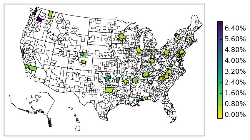
1     Introduction

At the end of 2015, housing represented 49.5% of the median-wealth household portfolio, largely

ahead of stocks (directly and indirectly held), which only represented 3.5% of the portfolio (Panel

Study of Income Dynamics Survey PSID, 2015). Even for households at the top 1% of the wealth

distribution, housing was larger than stocks (29.1% versus 25.2%).1 However, while numerous stud-

ies have investigated the cross-section of expected stock returns (e.g., Fama and French, 1992, 1993

and 2015; Carhart, 1997; Pastor and Stambaugh, 2003), the cross-section of expected housing re-

turns is still largely uncharted territory. In addition, homeownership generates under-diversification

because housing is lumpy and hence limits the ability of a household to invest in other asset classes

(e.g., Flavin and Yamashita, 2002; and Cocco, 2005). Further, households are typically limited in

the extent to which they can diversify the real estate component of their wealth portfolios. The

under-diversification associated with homeownership suggests that idiosyncratic risk should matter

in the housing market. But again, while idiosyncratic volatility has been extensively studied for

stocks (e.g., Goyal and Santa-Clara, 2003; Ang et al., 2006; Herskovic et al., 2016), idiosyncratic

housing risk has hardly been investigated.

    This paper fills these voids by performing an extensive zip code-level asset pricing analysis for a

large cross-section of 9,831 zip code-level U.S. housing returns from Zillow.2 As for commercial real

estate, there is a significant presence of diversified landlords (e.g., local-residential companies, large

apartment and single-family housing REITs, and individuals owning more than one property) in

the residential market.3 When diversified landlords and undiversified owner-occupants participate

in the same housing market, the degree of under-diversification is a function of this participation

and the relative pricing of systematic and idiosyncratic risk becomes an empirical question.4 A few

earlier studies have analyzed the risk-return trade-off in the housing market, but their focus has
    1
      It is at the very top of the households’ wealth distribution that stocks dominate housing (e.g., at the top 0.1%
of the wealth distribution, stocks represented 21.1% of the average portfolio compared to 18.0% for housing). These
figures are in line with those reported by earlier studies (e.g., Campbell, 2006; Guiso and Sodini, 2013; Barras and
Betermier, 2016).
    2
      Several papers have used zip code-level or other aggregation level data from Zillow to analyze mortgage defaults,
foreclosures, and household leverage (e.g. Mian and Sufi, 2009, 2011; Mian, Sufi and Trebbi, 2015; and Adelino,
Schoar and Severino, 2016).
    3
      Ioannides and Rosenthal (1994) document that about 23% of homeowners have more than one property.
    4
      Plazzi, Torous and Valkanov (2008) find a positive relation between idiosyncratic risk and expected returns on
commercial real estate, suggesting that owners of commercial real estate are not always well diversified.

                                                          1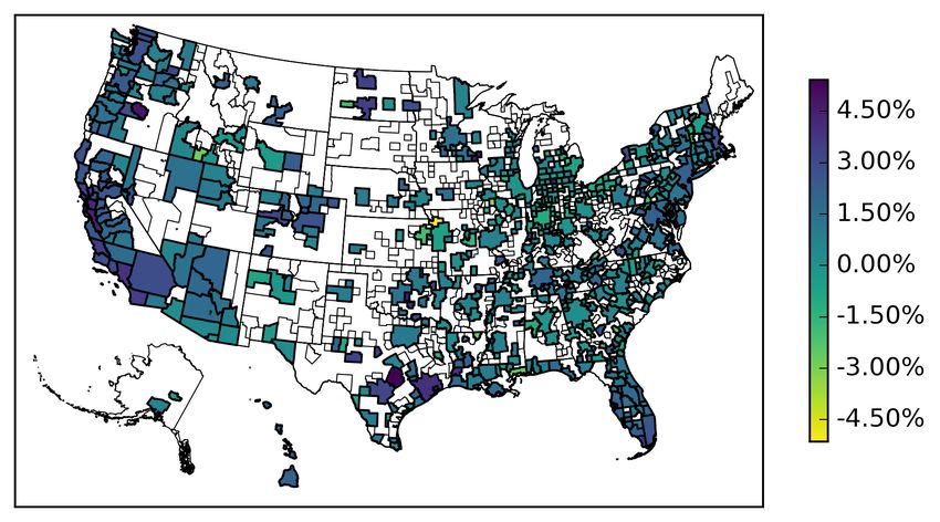
been exclusively on housing returns at the metropolitan statistical area (MSA) level.5 Our zip code-

level data allows us to estimate idiosyncratic risk at the zip code-level, which leads to important

new insights on the pricing of systematic and idiosyncratic risks and on the determinants of these

housing risk premia.

       We estimate risk exposures and prices of risk with respect to U.S. housing market returns

(national factor), MSA-level housing market returns (local factor), and equity market returns using

the Fama and MacBeth (1973) methodology. To estimate zip code-level idiosyncratic housing risk

(IVOL), we follow Ang et al. (2006) and take the standard deviation of the residuals from this

model. Because we have access to zip code-level housing returns, we can estimate our multifactor

model separately for each MSA. This allows us to provide new insights on an additional question,

one that is highly debated in the housing literature: the extent to which the U.S. housing market

is locally segmented.6

       Our sample consists of monthly housing returns for 9,831 zip codes across 178 Metropolitan

Statistical Areas (MSAs) from April 1996 to December 2016.7 To the best of our knowledge, we are

the first to consider monthly housing returns at this highly disaggregate level, covering a large part

of the U.S. housing market. We find striking differences across MSAs on whether a certain type of

risk is priced. Even though we focus on a minimum of only 15 zip codes per MSA, we find that, for

103 MSAs, at least one source of risk carries a significantly positive premium.8 This suggests that

the risk-return relationship in housing is important in the majority of MSAs. Specifically, U.S. and

MSA-level housing-market risks are positively priced in 47 and 39 MSAs, respectively. Notably, the

evidence that MSA-level housing-market risk is priced in roughly a fifth of the MSAs runs counter

to the common belief that the U.S. housing market is locally segmented. Both types of systematic
   5
     See, e.g., Case, Cotter and Gabriel (2011), Han (2013) and Cotter, Gabriel and Roll (2015). One exception is
Cannon, Miller and Pandher (2006), who also consider zip code-level housing returns. However, they only have eight
annual time series observations, which complicates asset pricing tests.
   6
     One possible reason for locally segmented housing markets is that if the local economy is in a downturn, housing
supply might increase (this may result, for instance, from households trying to relocate to markets with better
employment opportunities), while demand may decrease. In turn, this put a downward pressure on local-house
prices.
   7
     Our initial sample includes monthly-housing returns from Zillow for 12,243 zip codes across 571 Metropolitan
Statistical Areas (MSAs) from April 1996 to December 2016. However, to ensure that we have a sufficiently large
cross-section of housing returns, in our estimations of the multifactor model, we require each MSA to have at least
15 zip codes. Because of infrequent trading, time series of housing returns are not available at the property level.
Hence, we rely on the next best thing: zip code-level housing returns from Zillow.
   8
     When we allow for positive and negative risk premia estimates and we use a minimum of 20 zip codes per MSA,
we have a significant price of risk for 76% of all MSAs.

                                                         2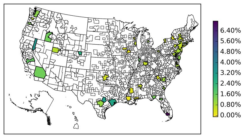
housing risk are positively priced in only eight of the MSAs. The equity market risk is positively

priced in just five MSAs, which suggests that it plays a marginal role in housing.

   Contrary to the expectation that idiosyncratic risk should be widely priced in the housing

market because homeowners typically own only one property (and hence hold undiversified real

estate portfolios), we find that it is positively priced in only 39 MSAs. Both idiosyncratic and

systematic (national and/or local) risks are priced in 19 MSAs.

   We make use of heat maps to help visualize whether there are systemic patterns in the pricing

of the different types of risks across regions. We find that the U.S. housing index is positively priced

in many large MSAs on the East Coast (e.g., New York and Philadelphia), the South (e.g., Austin

and Houston), and the West Coast (e.g., Seattle and Fresno), but also in several small MSAs across

the country. We further find that the average annualized risk premium across MSAs for the U.S.

housing index is 1.07%, which is sizable compared to the average MSA excess return of 0.86%. We

document similar patterns in the pricing of risk for the MSA housing index and idiosyncratic risk,

while, as discussed earlier, the equity market index is hardly ever priced. Overall, our analysis

suggests that U.S. housing index risk, MSA housing index risk, and idiosyncratic risk are priced

in a wide range of different-sized MSAs across the entire U.S., although smaller MSAs command

higher risk premiums.

   In the last part of the paper, we link MSA variation in the estimated prices of risk to MSA

fundamentals using probit regressions. MSA characteristics are obtained from multiple sources,

including Zillow, the U.S. Census and American Community Survey (ACS)-Integrated Public Use

Microdata Series (IPUMS), the Internal Revenue Service (IRS), and the Federal Housing Finance

Agencys Monthly Interest Rate Survey (MIRS). Housing-supply elasticity data are obtained from

Saiz (2010) and Gyourko, Saiz and Summers (2008). We find that U.S.-wide housing-market risk

is more likely to be priced in MSAs with relatively more illiquid housing markets, where liquidity

is measured as average (log) days on the market. MSA-level housing risk is more likely priced in

MSAs where homeownership rates are higher. In these areas, there are fewer renters and hence

fewer well-diversified landlords. Consequently, the marginal investor is more likely to be someone

exposed to local MSA-level housing risk, which then carries a risk premium.

   We also find that the probability of idiosyncratic risk being positively priced is lower in MSAs

                                                   3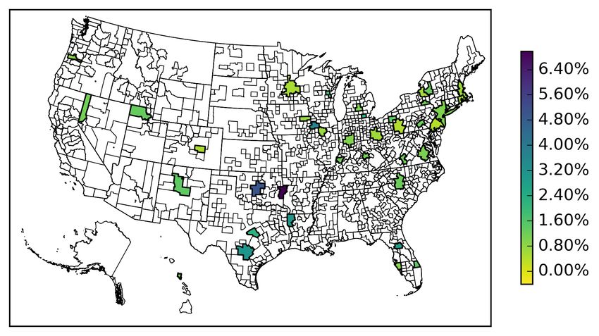
where market liquidity (measured as days-on-market) is higher. Further, we find that idiosyncratic

housing risk is less likely to be positively priced in MSAs with more undevelopable land. To the

extent that more undevelopable land makes it is easier for homeowners to sell existing properties,

these two findings suggest that under-diversification is less binding when liquidity is higher. Finally,

idiosyncratic risk is less likely to be priced for homeowners with strong-hedging incentives within

MSAs. In line with the insights in Sinai and Souleles (2005; 2013) and Han (2013), this result

suggests that homeowners are less concerned with under-diversification if homeownership is an

instrument to benefit from potential house price increases that can be used in the future for the

purchase of a larger house within the same MSA.

       In line with economic theory, we primarily focus on positive price of risk estimates. At the

same time, several studies have found negative premiums for idiosyncratic risk in the cross-section

of equity returns (e.g., Ang et al. 2006).9 Nevertheless, we find that for housing most of the

significant idiosyncratic risk premia are positive which suggests that the idiosyncratic risk puzzle

for equity returns does not extend to the cross-section of housing returns. Hence, our overall results

remain very similar when we allow for negative prices of risk.

       Our main findings pass a significant number of robustness tests. We find that our results hold

in the following conditions: 1) when we restrict the sample period to 1996-2007 to control for

the effects of the subprime crisis; 2) when we estimate our multifactor model for MSAs with a

minimum of 20 instead of 15 zip codes; 3) when we control for housing value and zip code size in

the estimation of our multifactor model; 4) when we estimate our multifactor model without the

stock market risk factor.

       Our paper relates to a growing literature on housing-market risk. Using MSA-level data, Cotter,

Gabriel and Roll (2015) find that, during the boom of the 2000s, a large proportion of MSA housing

returns is explained by a common set of variables (e.g., loan-to-value ratio, industrial production,

and Federal Funds rate), which suggests that MSA housing markets are highly integrated and

offer limited opportunities for diversification.10 Case, Cotter and Gabriel (2011) analyze the risk-
   9
     The empirical evidence for the pricing of idiosyncratic risk of stocks is mixed. Ang et al. (2006) find a strong
negative cross-sectional relationship between idiosyncratic volatility and expected stock returns. In contrast, Fu
(2009), and Huang et al. (2010) find a positive cross-sectional relationship. Conrad, Dittmar and Ghysels (2013) find
no significant cross-sectional risk-return relationship when estimating ex-ante idiosyncratic volatility from options.
Finally, Stambaugh, Yu and Yuan (2015) find a negative cross-sectional relationship for overpriced stocks, and a
positive relation for underpriced stocks.
  10
     In a recent study, Cotter, Gabriel and Roll (2018) document that integration within and among equity, fixed

                                                          4
return relation at the MSA level. Among other things, these authors find that, on average across
MSAs, risk exposure to the U.S. housing market and equity market are positively significant.
Cannon, Miller and Pandher (2006) estimate a single-factor model of housing exposure to the
equity market and find that equity risk and idiosyncratic risk are important in explaining the risk-
return relationship for the overall U.S. housing market. Han (2011; 2013) focuses on the puzzling
negative relation between total risk and return in the U.S. housing market. Using a panel regression
framework, this author finds that this relation can be explained by the hedging that homeownership
provides to households that intend to buy a larger house in the same MSA or a similar size house
in a different, but highly correlated MSA (as predicted by the theory in Sinai and Souleles, 2005).11
In our paper, we estimate a multifactor model with monthly zip code-level data. This allows us
to make four important contributions to the literature: 1) we measure idiosyncratic housing risk
at the zip code-level, which is the most disaggregated-level possible based on data availability; 2)
we pinpoint the risk factors (systematic and/or idiosyncratic) that are priced in each MSA; 3) we
identify the MSA characteristics that can help explain whether a certain risk exposure is priced;
and 4) we shed light on the degree of local segmentation of the U.S. housing market.
The rest of the paper is organized as follows. Section 2 discusses the multifactor models used
to estimate systematic and idiosyncratic risks in the housing market. Section 3 introduces the data
and presents descriptive statistics of all the variables. In section 4, we discuss the types of risk
priced and the magnitude of the estimated risk premia across MSAs. Section 5 relates the cross-
MSA variation in risk premia to MSA-level characteristics. Section 6 concludes. The Appendix
gives more details on the data sources and variables construction. An Online Appendix provides
details on data sources and variable constructions and reports the results of various robustness
tests.
income, and real estate (i.e., Real Estate Investment Trust) has increased significantly after 2000 both within and
among countries, pointing to diminished opportunities for diversification across asset classes and regions.
11
Our paper also relates to a stream of research linking housing returns to stock returns. Lustig and Nieuwerburgh
(2005) show that the ratio of housing wealth to human wealth predict future stock returns. Piazzesi, Schneider and
Tuzel (2007) find that the housing share of total consumption predicts future excess returns. Using a time series of
returns from 1870 to 2015 for several asset classes, Jordà et al. (2018) find that housing outperforms equity prior to
World War II, but the opposite occurs afterwards.
52 Empirical Framework
Our empirical analysis consists of two steps. First, we perform cross-sectional asset pricing tests
to analyze the pricing of systematic and idiosyncratic risk in the housing market. As we discuss in
detail below, we perform these tests for each local housing market (i.e., for each MSA) separately,
in order to allow for local risk factors and to be able to test whether housing markets are locally
segmented or not. In the second step, we analyze differences in the estimated prices of risk across
MSAs by linking them to MSA-level housing market and other economic fundamentals.
2.1 Multifactor Model for the Cross-Section of Expected Housing Returns
To analyze the cross-section of expected U.S. residential housing returns, we estimate multifactor
models using the Fama and MacBeth (1973) approach. While this is similar to the typical analysis
of the cross-section of expected U.S. stock returns, there are two important differences between the
stock market and the housing market that need to be taken into account.
First, there is evidence that housing markets cluster and local aspects matter (e.g. Goetzmann,
Spiegel and Wachter 1998, Cotter, Gabriel and Roll 2015). Therefore, rather than estimating a
single model for the entire cross-section of U.S. housing returns, we allow for local segmentation by
separately estimating an asset pricing model for each MSA. The model includes U.S.-wide housing
returns (and equity market returns) as well as local housing returns as risk factors. In contrast,
existing studies of housing returns (e.g. Case, Cotter and Gabriel 2011 and Cotter, Gabriel and
Roll 2015) only consider U.S.-wide housing and equity-market systematic risk factors.12 Thus, we
estimate a multifactor model separately for each of the 178 MSAs (with a total of 9,831 unique zip
codes) in our estimation sample.13
A second difference between the cross-section of stock returns and the cross-section of housing
returns is the potential role of idiosyncratic risk. While achieving a well-diversified stock portfolio
is straightforward, this is not the case for residential real estate. Homeowners often own only one
property which means they hold an under-diversified real estate portfolio (Flavin and Yamashita
2002 and Cocco 2005). Consequently, not only is systematic risk important for asset prices, but
12
Our approach follows the international finance literature where partially segmented models include both global
and local (regional or country-level) risk factors (see e.g., Bekaert, Hodrick and Zhang 2009).
13
This specification is also in line with Goetzmann, Spiegel and Wachter (1998), who find that zip code-level housing
returns tend to cluster with the return of the central city in their metropolitan area.
6idiosyncratic risk may also play a role (Merton 1987).
We deviate from existing papers that analyze housing returns (e.g., Case et al. 2011, Han
2013 and Cotter, Gabriel and Roll 2015) in two ways. First, we recognize that even though many
homeowners are under-diversified, better-diversified landlords are also active in the residential real
estate market. As we do not know who the marginal investor is, we allow for the possibility that
idiosyncratic risk is priced. We therefore include idiosyncratic volatility in our model, in addition
to the U.S.-wide and local systematic risk factors. In the second stage of our empirical analysis,
we relate the cross-MSA heterogeneity in the pricing of systematic and idiosyncratic risk to various
MSA-level fundamentals, such as the homeownership rate.
Second, to capture the idiosyncratic risk that under-diversified homeowners face, we need to
consider housing returns at the most disaggregated-level. We therefore use zip codelevel housing
returns. Ideally, one would like to estimate idiosyncratic risk at the individual house level. However,
for this purpose we would need a sufficiently large time-series of prices for each house. Even
transaction-level data from multiple listing services (MLSs) would not be suitable since transactions
data at the house level would only give us only a few observations during our roughly 20-year sample
period, and this would not allow us to run any type of time-series regression. This means that
monthly frequency zip codelevel data is, at this point in time, the best and most suitable dataset to
run our type of analysis of idiosyncratic risk across the entire U.S. housing market. Existing papers
generally focus on MSA-level housing returns (e.g., Case et al. 2011, Han 2013 and Cotter, Gabriel
and Roll 2015), which does not allow for an analysis of idiosyncratic housing risk. One exception
is Cannon, Miller and Pandher (2006), who study zip codelevel returns. However, they only have
a time-series of eight annual observations, which complicates asset pricing tests. Further, their
main focus is analyzing the pricing of equity risk across the entire U.S. housing market, rather than
within each MSA, which means they do not allow and cannot test for local market segmentation.
We apply the standard two-step Fama and MacBeth (1973) approach to estimate each mul-
tifactor model. In the first step, we estimate time-series regressions for each zip code to obtain
idiosyncratic risk and the exposures to the systematic risk factors. Given that our full sample
contains 20 years of monthly returns, we use rolling-window regressions based on the previous 48
months.14
14
Following Fama and MacBeth (1973) and Bali and Cakici (2008) among others we also estimate our model using
7Zip Code-Level Risk Exposure Estimation The time-series regression that we use to estimate
the factor exposures and idiosyncratic risk for each zip code i is given by
m mkt hi hi msa orthmsa
ri,s = αi,t + βi,t rs + βi,t rs + βi,t rj,s + εi,s , f or s = t − 47, ..., t, (1)
where ri,s denotes the time-s = t−47, ..., t zip code-level housing return in excess of the risk-free
rate. The risk-free rate is measured as the one-month Treasury bill rate. rsmkt and rshi are U.S.
orthmsa is the orthogonalized
stock market and U.S. housing index excess returns, respectively. rj,s
excess return for MSA j, which is the MSA to which zip code i belongs. We follow Bekaert, Hodrick
and Zhang (2009) and orthogonalize the MSA excess return with respect to the U.S. housing index
excess return using an ordinary least squares regression given by
msa
rj,t = µj + βj rthi + ηj,t , (2)
msa that we use in (1).
where the error term ηj,t is the orthogonalized version of rj,t
Following the literature on stock market idiosyncratic volatility (see Ang et al. 2006), we
estimate zip code-specific idiosyncratic risk as the standard deviation of the residuals from the
p
time-series regression of our multi-factor model specified in (1), that is IV OLi,t = var(εi,s ) for
zip code i.
Next, for each month, we run cross-sectional regressions for all zip-codes within each of the 178
MSAs to estimate prices of risk for each factor in a particular MSA.
MSA-Level Price of Risk Estimation To estimate the MSA-specific prices of risk for each
factor, for each MSA j we run the contemporaneous cross-sectional regression given by
ri,t = λ0j,t + λm m hi hi msa msa ivol
j,t βi,t + λj,t βi,t + λj,t βi,t + λj,t IVOLi,t + ξi,t , (3)
where we only include zip codes i that belong to MSA j and use the risk exposures and idiosyncratic
volatilities as estimated through (1) based on the previous 48 months. We run this cross-sectional
regression for each month t in the sample which yields a time-series of λkj,t for each type of risk k.
60 monthly returns. This limits our sample for the second-stage estimation of prices of risk. Nevertheless, our main
results and conclusions hold using this longer rolling window sample. These results are available upon request.
8The estimate of price of risk λkj for each risk factor is found by taking the time-series average of
the corresponding λkj,t . Finally, we test whether each average price of risk is different from zero.
2.2 Heterogeneity in the Pricing of Risk and Local Housing Market Fundamen-
tals
Our approach of estimating a multifactor model separately for each MSA will yield different esti-
mates of the prices of risk for each local housing area. We may also have differences across MSAs
on whether a price of risk is significant. For instance, we may find that in some MSAs, idiosyncratic
risk is priced, while in others, only systematic risk matters. To better understand the why risk
factors are priced in some MSAs but not in others, in the second step of our empirical analysis,
we investigate which MSA characteristics help explain cross-MSA differences in the pricing of risk.
For this purpose, we estimate a probit regression in which the dependent variable δt is an indicator
equal to one if the price of risk is positive and significant, and zero otherwise. The probit regression
is given by
P r(δt ) = α + Zt| β + εt
We estimate this model separately for each of the estimated prices of risk of the U.S. housing
index, the local MSA return and IV OL. Since we estimate unconditional factor models, we can
only explore cross-MSA differences in estimated prices of risk. Therefore, as independent variables
Zt in the probit regressions, we include time-series averages of the fundamental economic variables
discussed in the next section.
3 Data and Descriptive Statistics
In this section we introduce the data and present descriptive statistics of all quantities used in the
empirical analysis.
93.1 Asset Pricing Analysis Data
The data for residential housing prices are obtained from Zillow. They provide the Zillow Home
Value Index (ZHVI) at a monthly frequency for different aggregation levels ranging from zip code-
level to state-level. The ZHVI is based on estimates on the market value of individual homes that
Zillow calls Zestimates. Since our framework allows for idiosyncratic risk to be priced, we focus
on the lowest aggregation level available, namely zip code-level data. We merge the zip code-level
data with the MSA-level ZHVI data. After merging these datasets, we are left with 12,243 unique
zip codes and 571 unique MSAs for the sample period April 1996-December 2016.15 Zillow also
provides the ZHVI for the entire U.S. residential housing market, which we use in our empirical
analysis as a proxy for U.S. housing market prices.16 To compute housing excess returns we subtract
the one-month Treasury bill rate. These data as well as data on monthly U.S. stock-market excess
returns are obtained from the online data library of Kenneth R. French.17
The zip code-level data from Zillow does not cover all zip codes in each MSA. To obtain a
measure of how well the observed zip codes cover each MSA, we obtain population data per zip
code from the 2010 U.S. Census. We merge this data with the Zillow zip code-level data and
compute the population per MSA. We then compare this population in relation to the reported
MSA total population from the 2010 U.S. Census. We find that, on average, the Zillow zip code-
level data covers 86.5% of total MSA population, with the median coverage being 91.6%. The
Zillow zip code data thus provides good coverage for each MSA.
3.2 MSA-level Fundamental Housing Market and Other Economic Data
In our empirical analysis we not only estimate prices of risk and risk premia, but we also investigate
MSA characteristics that can help explain cross-MSA heterogeneity in the pricing of risk. To
this end, we combine multiple datasets to construct various MSA-level housing market and other
economic variables. Below, we discuss the variables by data source.
15
The 2008 financial crisis falls in the middle of our sample period, and this was a turbulent period for house prices.
Therefore, as a robustness check, we end the sample in 2007 for our empirical analysis (see Section 4.4)
16
Appendix A.1 provides a detailed description on how we merge the different ZHVI geographies.
17
http://mba.tuck.dartmouth.edu/pages/faculty/ken.french/data library.html
10Zillow Data We obtain days-on-market at the MSA-level from Zillow, which we use as a liquidity
measure in our empirical analysis. The data is available for the full sample period.
MIRS Data We obtain data on zip code-level loan-to-value ratio (LTV) from the Federal Housing
Finance Agency’s Monthly Interest Rate Survey (MIRS) for the full sample period. The MIRS
covers a large sample of zip codes for our entire sample period. We first merge this data with
Zillow zip code data to obtain MSA identifiers, since our goal is to aggregate it to the MSA level.
Notably, for some months, the MIRS data contains several LTV values for the same zip code. We
choose take the mean LTV for each zip code. Using the zip code-level LTV, we then aggregate it
MSA-level by taking the median LTV across zip codes within each MSA. This way, we avoid any
data errors or outliers when calculating the MSA-level monthly LTV ratio.18
IRS Migration Data Among our MSA characteristics are measures of across-MSA and within-
MSA hedging incentives first introduced by Han (2013). These measures capture both the likelihood
that households within their local MSAs will trade up to a bigger house in the future, and the
correlation between the local housing market and the market where they plan to move.19 Both of
these measures require data on MSA-to-MSA household migration. Following Sinai and Souleles
(2013), we use county-to-county migration data obtained from the Internal Revenue Service (IRS),
which is aggregated to MSA-to-MSA migration. The IRS provides yearly data on county-to-county
migration and we obtain this data for the period 1996-2016. Unfortunately, the IRS does not
provide the MSA identifier for each county. To obtain MSA identifiers for each county, we merge
the IRS county-to-county migration data with the county-level Zillow data as this data includes
an MSA identifier for each county. Since we are interested in MSA-to-MSA migration, in the next
step, we retain only MSA-to-MSA pairwise migration. This data then allows us to calculate the
number of people that stayed in each MSA every year, which is a key component in the within-MSA
hedging incentive indicator. This pairwise migration data is also needed to compute weights for the
estimation of expected correlations, which are key components of the across-MSA hedging incentive
variable.
18
In our empirical tests, we also use the mean LTV across zip codes as a measure of MSA-level LTV. We find
similar results using this measure and these are available upon request.
19
A detailed description on the construction of both the expected correlation and hedging incentive variables from
Han (2013) and Sinai and Souleles (2013) can be found in Appendix A.2.
11IPUMS Data We use individual data from the U.S. Census and American Community Sur-
vey (ACS) obtained through the Integrated Public Use Microdata Series (IPUMS) database (see
Ruggles et al. 2017). The IPUMS consists of more than 50 high-precision samples of the Amer-
ican population drawn from 15 federal censuses and from the American Community Surveys of
20002012. Geographically, we follow the 2013 definitions of MSAs from the U.S. Office of Manage-
ment and Budget (OMB). Our IPUMS dataset consists of 255 MSAs and has annual data for the
period 20002016. The IPUMS data we use covers household total income, population, homeown-
ership, fraction of population aged 20-45, and rental costs. To obtain MSA-level data, we compute
means, medians, and standard deviations across households within each MSA-year combination,
applying household weights to properly incorporate the stratified sampling scheme. The fraction
of population aged 20-45 is used to construct the hedging incentive variables.
BLS Data Monthly values of the consumer price index (CPI) are from the Bureau of Labor
Statistics (BLS). These data are obtained for our full sample, which runs from April 1996 to
December 2016. We use this data to deflate rental costs and construct a measure of real rent
volatility following Sinai and Souleles (2005).
Housing Supply Constraint Data We also obtain data on local-housing supply constraint
measures. In particular, we use the share of undevelopable land from Saiz (2010), and the Wharton
Residential Land Use Regulation Index (WRLURI) from Gyourko, Saiz and Summers (2008). We
obtain these measures directly from the authors. The data lacks a time series dimension as these
measures are available for the cross-section of MSAs in one particular year. Saiz (2010)’s measure
of the share of undevelopable land is not expected to change much over time as it is estimated by
satellite-generated data on terrain elevation and presence of water bodies. Geographical terrain
does not significantly change in such a short period. The WRLURI is comprised of 11 subindices
based on the local regulatory environment of each MSA in 2008.
3.3 Descriptive Statistics
In Table 1, we present a set of summary statistics for excess housing returns at the zip code,
MSA and U.S. level, as well as U.S. stock market excess returns. These include the number of
12observations, mean, median, minimum, maximum, and standard deviation. All statistics are based
on annualized excess returns. For the zip code-level and MSA-level excess returns we also report
the dispersion across MSAs. Excess returns are computed by subtracting the one-month Treasury
bill rate. For this part of the analysis, we consider the full sample of 12,243 zip codes across 571
MSAs.
[Insert Table 1 here]
The zip code-level statistics, except the cross-sectional dispersion, are computed in three steps.
First, we take the time-series statistic for each zip code. Second, within each MSA we take the
cross-sectional mean of these statistics. Finally, we take the average across MSAs. The cross-
sectional dispersion measure is computed by first taking the time-series mean for each zip code,
next we compute the average within each respective MSA, and finally we take the cross-sectional
standard deviation across MSAs.
The MSA-level statistics, except the dispersion, are computed in two steps. First, we take
the time-series statistic for each MSA. Then, we take the cross-sectional mean of these time-series
statistics. The dispersion measure is computed by first taking the time-series mean of each MSA,
and then taking the standard deviation of these time-series means.
As expected, we find that zip code-level excess housing returns are more volatile than both
MSA- and U.S.-level excess housing returns. The standard deviations are 12.73%, 9.63% and
5.39% per annum, respectively. The zip code-level average excess return (0.84%) is lower than both
the average MSA (0.86%) and U.S. housing index (1.07%) excess housing returns.20 Finally, the
U.S. stock market has both a higher average yearly excess return (7.95%) and a higher standard
deviation (18.76%) than housing returns for any aggregation level.
[Insert Figure 1 here]
In Figure 1 we plot a geographical heat map of the U.S. and highlight the range of average yearly
excess returns for all 571 MSAs present in our sample. In line with our expectations, we see that
the highest excess returns (shown in purple) are mostly found in Californian MSAs. California has
had a large increase in house prices in recent years. On the East Coast we see large excess returns
20
Note that the averages are equally weighted across zip codes and across MSAs. Therefore, we cannot directly
compare these averages based on disaggregate data to U.S.-wide housing returns.
13in the largest MSAs, including New York. Some smaller MSAs such as Syracuse, NY had excess
returns close to zero. We also see very few MSAs with negative average excess returns, and in
general these MSAs are small (e.g. Albany, GA, Bennington, VT, and Chambersburg, PA).
[Insert Figure 2 here]
In Figure 2 we plot a geographical heat map of the U.S. and highlight the range of average yearly
excess returns for all 12,243 zip codes in our sample. As expected, based on the MSA excess returns,
we find that many of the highest excess returns can be found in zip codes in Los Angeles and San
Francisco, CA on the West Coast, and New York, NY on the East Coast.21
[Insert Table 2 here]
In Table 2, we present a set of summary statistics for MSA-level characteristics listed in Section 3.2.
In the second part of our empirical analysis, we will use these variables to help explain cross-MSA
variation in estimated risk premia. Here, we briefly discuss their summary statistics in order to
gain more insight into the characteristics of the local housing markets under consideration.
Note that the most of MSA-level characteristics are available for a smaller set of MSAs than
in the Zillow MSA-level housing price data. For the full sample of 571 MSAs, we can match
characteristics for 214 up to 534 MSAs. At the same time, for our empirical analysis we require a
cross-section of at least 15 zip codes per MSA to be able to estimate prices of risk for that MSA.
Table 2 shows that the average number of zip codes per MSA varies widely. While the average
number of zip codes across MSAs is 21.44, the median is nine, with a minimum of one and a
maximum of 736 zip codes. The constraint of at least 15 zip codes implies that we are can perform
the asset pricing tests for 178 MSAs. We can match all characteristics for 118 of them.
The population across MSAs varies widely as we have very large MSAs (e.g., New York) to
much smaller MSAs (e.g., Syracuse). The share of undevelopable land is, on average, 25.86% with
a median of 18.60%. Both these values are in line with Saiz (2010). Our sample of MSAs has
a notably broad range of shares of undevelopable land with a minimum of 1.04%, a maximum of
86.01%, and standard devation of 21.05%. This means that in some MSAs, almost all available land
21
For 2017, 77 of the 100 most expensive zip codes for housing in the U.S. were found in California,
see e.g. http://www.latimes.com/business/realestate/hot-property/la-fi-hotprop-propertyshark-zip-codes-20180117-
story.html.
14is developable, while in others, less than 20% of the available land can be used for housing. Our
measure of local housing regulations WRLURI has a negative mean of -0.08 and a median of -0.15.
These are in line with Gyourko, Saiz and Summers (2008). The original WRLURI is constructed
to have a mean of zero and a standard deviation of one. The negative average and median in our
sample indicate that the median MSA is less regulated than the average MSA. Further, we see a
broad range of values for the WRLURI in our sample of MSAs, with a minimum of -1.76 and a
maximum of 3.12, with a standard devation of 0.78. Our sample thus contains both highly locally
regulated and relatively unregulated MSAs. The average homeownership rate across our MSAs
is 67.83% with a broad range of values and a high dispersion across MSAs of 6.22%. Volatility
of real rents is on average 4.64%, with a slightly lower median of 4.09%. The average number of
days-on-market for listed houses in our sample of MSAs is roughly 114 days, but liquidity varies
widely across our MSAs with a minimum of 51 days and a maximum of roughly 219 days. Our
sample thus includes both liquid and illiquid local housing markets. The fraction of the population
aged 20-45 is on average 35.42%, with a similar median and a low dispersion across MSAs of 3.53%.
Thus, most MSAs in our sample have a similar number of relatively young households.
The mean within (across) -MSA hedging indicator is 0.50 (0.47), which implies that about 50%
(47%) of local housing markets have strong hedging incentives. The average across-MSA hedging
indicator is in line with Han (2013) but the within-MSA hedging indicator is slightly lower. This
could be explained in part by the fact that we have a different sample of MSAs, and a different
sample period. Most importantly, we use detailed migration data from the IRS to create this
variable. In contrast, Han (2013) uses IPUMS migration data which is only available once every
ten years (i.e., 1990, 2000 and 2010), and assumes that it stays constant in between. As the IRS
migration data is yearly we do not need to assume constant mobility rates within a decade.
Expected correlation is a measure of the correlation between the housing market where house-
holds currently reside and the housing market where they plan to move. Our mean expected
correlation is 0.35, which is lower than the mean of 0.57 found in Sinai and Souleles (2013). How-
ever, if we restrict our MSA sample to match Sinai and Souleles’s 44 MSAs (of which we can match
39 to the Zillow data) we find a similar mean, 0.53 versus 0.57, respectively.
154 Empirical Asset Pricing Results
The first step of our empirical analysis is to estimate the multifactor asset pricing model for each of
the 178 MSAs in our estimation sample. This means that we perform cross-sectional asset pricing
tests for 178 different cross-sections. As discussed in Section 2, our model includes U.S.-wide housing
market and equity market returns, MSA-level housing returns and zip code-level idiosyncratic
volatility. Hence, our framework allows for the pricing of systematic and/or idiosyncratic risk.
Further, our framework also allows us to test whether markets are locally segmented or not.
4.1 Risk Exposure Estimation
We first examine the estimated zip code-level factor exposures and idiosyncratic volatilities (IV OL),
which are based on rolling window regressions based on Equation (1) at the zip-code level using
48 monthly returns. Table 3 presents descriptive statistics of the risk exposures (betas) and the
IV OL estimates of the first-stage time-series regressions. All statistics are computed in two steps.
First, we take the time-series average of the monthly factor exposures and IV OL for each zip code.
Second, we take cross-sectional statistics of these time-series means.
[Insert Table 3 here]
We have sufficient time series observations to run the regressions for all of the 12,243 unique zip
codes except two. In Panel A, we report descriptive statistics for the entire sample. Panel B reports
the same statistics for our estimation sample used in the cross-sectional regressions. As explained
in the previous section, the estimation sample consists of the 178 MSAs with at least 15 zip codes,
resulting in a total of 9,831 zip codes.22
Consistent with existing literature (see e.g., Case and Shiller 1989, and Jordà et al. 2018) in
both panels we find that the average U.S. stock market exposure β m is essentially zero with a
mean (median) of -1.2e-3 (-9.0e-4) and -1.3e-3 (-1.0e-3), respectively. This implies that owning
a house does not generate exposure to stock market risk. Consequently, combining residential
real estate with stocks can potentially lead to substantial diversification benefits.23 Nevertheless,
22
In Section 4.4, we perform our asset pricing tests including only MSAs with at least 20 zip codes and find similar
results.
23
In the robustness tests discussed in the following section, we exclude the equity market factor and find very
similar results.
16Cotter, Gabriel and Roll (2018) find declining diversification benefits after 2000 across a range of
assets including equity, debt and real estate within and across countries.
A one-factor model for housing returns including only the U.S. housing index would be similar
to a CAPM for stock returns, and the CAPM predicts an (weighted) average stock market beta
equal to one. In both the full and the estimation sample, we find that indeed the average U.S.
housing index beta is close to one at 0.92 and 0.97, respectively. The beta does vary substantially
across MSAs, as indicated by the cross-MSA dispersion of 0.75. Further, we find that zip code-level
housing returns carry a substantial exposure to local MSA-level housing returns (orthogonalized
with respect to U.S.-wide housing returns). The mean (median) β msa is 0.72 (0.74) and 0.71 (0.75)
in the two panels. These beta estimates are relatively less dispersed with a cross-MSA standard
deviation of 0.41 and 0.43, respectively. These results suggest that allowing for locally segmented
housing markets may be important. However, to fully address the issue of market segmentation,
we need to estimate prices of risk, which we do in the next section.
The monthly IV OL has a mean (median) of 0.60% (0.53%) and 0.58% (0.51%) in the full and
estimation samples, respectively. The dispersion across MSAs is 0.29% and 0.30%, respectively.
To understand these values in relation to total risk, we also compute the rolling window standard
deviation of zip code excess returns as a proxy for total risk (volatility). To be consistent with
our estimation of IV OL, we use 48 months rolling windows. In comparison, the monthly total
volatility has a mean (median) of 0.82% (0.76%) and 0.78% (0.73%) respectively for our full and
estimation samples. We compute the ratio of IV OL to total volatility to see the share of total
risk that IV OL represents. We find that on average (median) across zip codes IV OL represents
75.36% (77.41%) and 76.04% (78.16%), respectively, of total volatility. This means that IV OL
represents roughly 75% of total risk in the housing market. This resonates with the stock market
idiosyncratic volatility literature, which finds that stock volatility consists mostly of idiosyncratic
volatility (e.g., Ang et al. 2009). Nevertheless, systematic risk still represents roughly 25% of total
risk. These results point to the fact that it is crucial to decompose total risk into systematic and
idiosyncratic risk, and analyze each risk separately in order to get a full picture of housing-market
risk. Notably, this variance decomposition does not necessarily imply that idiosyncratic risk is
priced. To draw conclusions about the sources of risk that drive expected housing returns, we need
17to perform second-stage Fama-Mac Beth cross-sectional regressions. We discuss those results in
the following section.
4.2 Estimation of Prices of Risk
We estimate MSA-specific prices of risk for each risk factor by running the cross-sectional regression
specified in (3) within each of the 178 MSAs in our estimation sample, using the risk exposures as
estimated in Section 4.1.
Asset pricing theory predicts that the price of market risk is positive. In line with this, we choose
to focus on positive prices of risk for all our types of risk and perform single-sided statistics tests.
Furthermore, in Section 5 we link these positive risk premia estimates to economic fundamentals.24
First, Table 4 presents descriptive statistics for the estimated prices of risk.
[Insert Table 4 here]
We report the number of MSAs that have significant positive prices of each risk at a 10% significance
one-sided level using Newey-West standard errors with two lags. We also report the average price
of risk and the dispersion across MSAs. We then look at how many MSAs have two, three or all
significant prices of risk.
U.S. Stock Market For the stock market return, we find that out of 178 estimated MSAs only
five (2.81%) have positive and significant U.S. stock market price of risk estimates, with an average
price of risk of 0.21 per annum, and a dispersion of 0.93. These findings, coupled with our previous
results showing that the U.S. stock market beta is close to zero for zip code-level housing returns,
suggests that the U.S. stock market risk plays a negligible role in the pricing of the cross-section of
residential housing returns.
U.S. Housing Index For the housing index return, we find that out of 178 estimated MSAs,
47 (26.40%) have significantly positive U.S. housing index prices of risk. The average price of risk
across MSAs is 0.01 per annum with a dispersion of 0.04. Previously, we found that the average
U.S. housing index beta in our estimation sample was, at 0.97, remarkably close to 1. These two
24
In Section 4.4 we relax this assumption, allow prices of risk to be both positive and negative, and find similar
results.
18results imply that U.S. housing risk is relevant for the cross-section of residential housing returns.
Note that based on pure chance, we could expect to find significant price of risk estimates in 10%
of the MSAs, and 26.40% surpasses this threshold level.
Local MSA Return For the local MSA housing risk factor (orthogonalized with respect to
the U.S. housing return), we find that out of 178 estimated MSAs, 39 (21.91%) have significantly
positive local MSA return prices of risk, with an average of 0.01 per annum and dispersion of 0.06.
This result shows that housing markets are not always locally segmented, as in roughly 78% of
MSAs local risk is not priced.
Idiosyncratic Volatility For IV OL we find that out of 178 estimated MSAs, 39 (21.91%) have
significantly positive IV OL prices of risk. The average IV OL price of risk is 2.05 per annum
with a dispersion of 9.93. This means that in roughly 78% of our estimated MSAs, idiosyncratic
risk is not priced. This finding stands in contrast to the argument that IV OL should be widely
priced in the housing market because homeowners typically own only one property (and hence hold
under-diversified real estate portfolios).
Factor Pricing Patterns In the bottom panel of Table 4, we report the number of MSAs that
have one or more significant prices of risk. We find that 78 MSAs have either λmsa or λhi significant,
which means that in 43.82% of our MSAs systematic risk (local or national) matters. Furthermore,
in 69 and 76 MSAs, respectively, we find that either λmsa or λivol , or λhi or λivol are significant,
which means that in 38.76% or 42.70% either systematic or idiosyncratic risk matters. We also
note in 101 MSAs either λmsa or λivol or λhi is significant, which means that 56.74% of MSAs have
systematic or idiosyncratic risk priced.25 While we find that at least one of the type of risks is priced
in a majority of our MSAs, it is interesting to see how many MSAs have both type of risks priced.
We find that only eight MSAs have both local and national risk priced, which represents 4.49% of
all estimated MSAs. Further, we find that just nine or 10 MSAs have both systematic (λmsa or
25
When we impose a minimum of 20 zip codes per MSA and we allow for both positive and negative price of risk
estimates, we find that for 77% of MSAs there is at least one source of risk that carries a significant risk premium.
This suggests that the lack of statistical significance may in some MSAs be related to the relatively small cross-section
of zip codes. At the same time, when we set the minimum at 20 zip codes, we lose a number of smaller MSAs. The
results of this robustness check are discussed in Section 4.4. Furthermore, when we link the risk premia estimates to
economic fundamentals, we control for the number of zip codes within each MSA.
19λhi ) and idiosyncratic (λivol ) risk priced, which represents 5.06% and 5.62% of all estimated MSAs,
respectively. Finally, only three MSAs have all three types of risk priced, which represents just
1.69% of all estimated MSAs.26 In the bottom of Table 4 we show that while we observe 178 MSAs
with at least one month of estimated price of risk, we find that 103 (57.87%) have one or more
significant prices of risk, 48 (26.97%) have two or more, 11 (6.18%) have three or more and none
have all four significant prices of risk.27
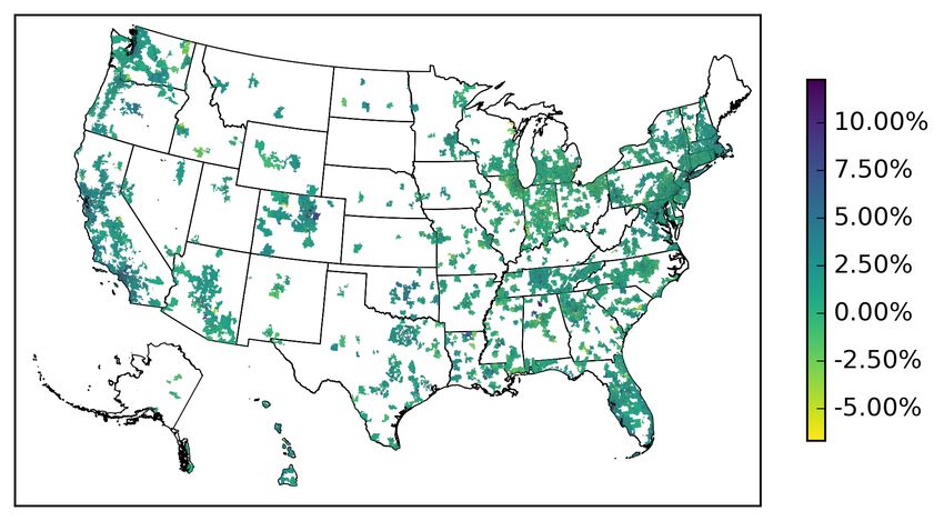
To investigate patterns in the pricing of risk across the U.S., in Figures 3a, 4a, 5a and 6a we
plot geographical heat maps of the U.S. and highlight in purple MSAs where the each respective
price of risk is positive and significant, and in yellow MSAs where each respective price of risk is
not significant.
[Insert Figures 3a and 4a here]
In Figure 3a we see that the U.S. stock market is not significantly priced in the majority of our
MSAs. On the other hand, in Figure 4a we see that the U.S. housing index is positively priced
in many East Coast MSAs, including New York and Philadelphia. It is also priced in some large
southern U.S. MSAs such as Austin and Houston. In the West Coast, we see that the U.S. housing-
market risk is priced in Seattle and Fresno. While the U.S. housing-market risk is priced in many
large MSAs, it is also priced in several small MSAs across the country such as e.g. Cedar Rapids,
IA, Salem, OR, and Savannah, GA, among others. These results show that the U.S. housing index
is priced in a wide range of different sized MSAs across the U.S.
[Insert Figure 5a here]
In Figure 5a we see that the local MSA return is priced in a broader set of MSAs that are located
all throughout the country, including Charlotte, Chicago, Dallas and Philadelphia. However, we
also see that the local MSA return is priced in many smaller MSAs (e.g.,San Luis Obispo, CA,
Yakima, WA, and Watertown, NY). Thus, we also find that the local MSA return is priced in wide
range of different sized MSAs across the U.S. This finding is in line with earlier papers showing that
housing markets cluster and that local aspects matter for housing returns (Goetzmann, Spiegel and
26
These three MSAs are Cedar Rapids, IA, Oklahoma City, OK and Philadelphia, PA.
27
In untabulated results, we find that, on average across MSAs, this three-factor model including idiosyncratic
volatility explains 27.99% of the cross-sectional variation in zip code excess returns.
20Wachter 1998). Nevertheless, in many of our estimated MSAs we do not find evidence of locally
segmented markets.
[Insert Figure 6a here]
Finally, in Figure 6a we find that IV OL is priced in many large East Coast MSAs, including Boston,
New York and Philadelphia. IV OL is also priced in a few large MSAs in the southern part of the
U.S. including San Antonio. While we see that IV OL is positively priced in many East Coast
MSAs, it is also priced in several large MSAs throughout the U.S. including Charlotte, Pittsburgh,
Minneapolis-St. Paul, and Columbus. Further, IV OL is also priced in small MSAs across the U.S.
(e.g. Appleton, WI, Ocala, FL, Peoria, IL, and Utica, NY). These results also suggest that IV OL
is priced in a wide range of MSAs across the entire U.S.
Prices of Risk and Risk Premiums While in Table 4 we present descriptive statistics of
prices of risk, in Figures 3a, 4b, 5b and 6b we focus instead on the risk premia associated with
each type of risk. For this purpose, we plot geographical heat maps of the U.S. and highlight the
range of annualized risk premia for each type of risk in MSAs where the respective price of risk is
significant.28
[Insert Figures 3b, 4b, 5b and 6b here]
In Figure 3b we see that in the very few MSAs where the U.S. stock market has a positive significant
price of risk, the risk premium is relatively low ranging from 0.15% to 1%. In Figure 4b we see
that in the majority of MSAs the U.S. housing index risk premium is economically large, ranging
from 2.40% to 4.00%, while the highest risk premium is found in Naples, FL at 7.13%. For the
local MSA return risk premium, Figure 5b shows that the values are somewhat lower, with the
majority of MSAs having an annualized risk premium ranging between 1.60% to 3.20%, while the
highest risk premium is found in Yakima, WA at 6.93%. Finally, Figure 6b shows IV OL has an
annualized risk premium in the majority of MSAs ranging from 3.20% to 4.80%, with the highest
risk premium found in Fort Smith, AR at 6.98%.
28
The risk premium for each risk is calculated in several steps. First, we calculate the time-series average beta for
each zip code. Second, we multiply each zip codes average beta with the estimated price of risk for the respective
MSA. Finally, we take the average across zip codes within each respective MSA. Risk premia are annualized by
multiplying by 12.
21[Insert Figure 7 here]
In Figure 7 we plot the average annualized risk premium across MSAs for each type of risk, as well
as the total risk premium composition. We also include the number of MSAs where each risk is
significantly priced. We see that the IV OL risk premium is the largest, on average between 1.55%
and 2.05%. The local MSA return risk premium commands the second highest with an average
between 0.88 and 1.15%, while the U.S. housing index has an average risk premium between 0.48%
and 1.06%. All three risk premia are large compared to the average annual MSA-level excess
return of 0.86% as seen in Table 1. In particular, the average yearly IV OL risk premium is almost
twice the size of the average MSA-level excess return.29 Finally, we see that the IV OL yearly risk
premium is largest in MSAs where all there risks are priced and constitutes more than half of the
total risk premium in these MSAs. On the other hand, we see that in MSAs where more than one
risk is priced, the U.S. housing index commands a low risk premium and constitutes a small part
of the total risk premium.
We saw in Table 3 that IV OL commands roughly 75% of the total risk at the zip code-level.
Since idiosyncratic risk represents on average the largest part of total risk, it is not surprising that
we find that it also commands the highest risk premium in MSAs where it is significantly priced.
Further, given the relative importance of idiosyncratic versus systematic risk, as well as local versus
national risk, our results also suggest that when analyzing the risk-return relationship in the cross-
section of residential housing returns, it is crucial to not only decompose total risk into systematic
and idiosyncratic risk but also to allow for local and national systematic risk.
[Insert Table 5 here]
4.3 Negative Prices of Risk
In line with asset pricing theory, throughout our main analysis we analyze only positive prices of
risk. In Table 5 we relax this assumption and allow prices of risk to be either positive or negative.
We find that the majority of U.S. housing index, local MSA return, and IV OL prices of risk are
positive. U.S. housing risk is significantly priced in 41 MSAs, with 34 (83%) carrying positive
29
Note, that this is not a perfect comparison since the average excess return from Table 1 is across all 571 MSAs
in the full sample, while the average IV OL risk premium is only for MSAs in which this price of risk is significant.
22You can also read