Mathematical Model of Freezing in a Porous Medium at Micro-Scale
←
→
Page content transcription
If your browser does not render page correctly, please read the page content below
Commun. Comput. Phys.                                                     Vol. 24, No. 2, pp. 557-575
doi: 10.4208/cicp.OA-2017-0082                                            August 2018

Mathematical Model of Freezing in a Porous Medium
at Micro-Scale
Alexandr Žák1, ∗ , Michal Beneš1 , Tissa H. Illangasekare2 and
Andrew C. Trautz2
1 Department of Mathematics, Faculty of Nuclear Sciences and Physical Engineering,
Czech Technical University in Prague, Trojanova 13, Praha, Czech Republic, 120 01.
2 Center for Experimental Study of Subsurface Environmental Processes, Colorado

School of Mines, Golden, Colorado 80401, USA.

Received 4 April 2017; Accepted (in revised version) 3 November 2017

           Abstract. We present a micro-scale model describing the dynamics of pore water phase
           transition and associated mechanical effects within water-saturated soil subjected to
           freezing conditions. Since mechanical manifestations in areas subjected to either sea-
           sonal soil freezing and thawing or climate change induced thawing of permanently
           frozen land may have severe impacts on infrastructures present, further research on
           this topic is timely and warranted.
               For better understanding the process of soil freezing and thawing at the field-scale,
           consequent upscaling may help improve our understanding of the phenomenon at the
           macro-scale.
               In an effort to investigate the effect of the pore water density change during the
           propagation of the phase transition front within cooled soil material, we have designed
           a 2D continuum micro-scale model which describes the solid phase in terms of a heat
           and momentum balance and the fluid phase in terms of a modified heat equation that
           accounts for the phase transition of the pore water and a momentum conservation
           equation for Newtonian fluid. This model provides the information on force acting on
           a single soil grain induced by the gradual phase transition of the surrounding medium
           within a nontrivial (i.e. curved) pore geometry. Solutions obtained by this model show
           expected thermal evolution but indicate a non-trivial structural behavior.

AMS subject classifications: 74N20, 74F10, 76S05, 80A22

Key words: Freezing, mechanics, phase-transition, soil, micro-scale.

∗ Corresponding author.
                      Email addresses: alexandr.zak@fjfi.cvut.cz (A. Žák),
michal.benes@fjfi.cvut.cz (M. Beneš), tillanga@mines.edu (T. H. Illangasekare),
atrautz@mines.edu (A. C. Trautz)

http://www.global-sci.com/                        557                       c 2018 Global-Science Press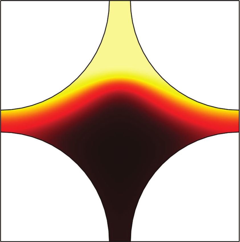
558                                   A. Žák et al. / Commun. Comput. Phys., 24 (2018), pp. 557-575

1 Introduction
Improved understanding of the thermal, mechanical, and wetting behavior of soil or
rock mass during freezing or melting is needed to address emerging environmental and
industrial problems. These problems include: the design and maintenance of structures
[1,2] in regions suffering from substantial temperature fluctuations; the exploitation of oil
and gas resources in cold regions [3]; the underground storage of liquefied petroleum or
natural gas within rock caverns [4], and the leakage of methane or carbon dioxide from
melting permafrost into the atmosphere [5, 6].
    A review of the literature related to these problems suggests that freezing-thawing be-
havior involves many complex processes (occurring during temperature shifts on the ma-
terial surface) which consist of several effects that arise from the bulk nature of each ma-
terial component, the interfacial interaction of the components, and the porous structure
of the material. Individual effects can be identified as: (i) the temperature dependence of
thermal and mechanical properties of constituents; (ii) the abrupt volume change during
the phase transition of the wet medium; (iii) the surface tension between different phases;
(iv) the drop of the freezing point of water associated with the surface tension effects; (v)
the drainage of water pushed out of the freezing zones into air voids; (vi) the swelling
of the soil material during freezing due to the suction of liquid water from unfrozen to
frozen regions and the consequent growth of the ice mass; (vii) the movement of the ice-
liquid interface during the cooling or warming of the material; (viii) the movement of
the ice body; (ix) the opening of microcracks during freezing and the collapse of the void
spaces during melting. Each of these effects contribute to the overall behavior differently
under different conditions that are dependent primarily on the type of thermal setting
(uniform or under a thermal gradient), its rate, soil material saturation, kind of soil/rock
material, porosity, etc.
    So far, several models have been developed that only partly describe the freezing-
thawing behavior. They are usually created for specific scenarios under which some par-
tial effects are allowed to prevail, and others neglected. This can be seen in the case
of models that only consider the heat balance during the freezing and thawing pro-
cesses [7, 8]. Other models deal solely with the frost heave [9–11], the upward move-
ments of saturated soil with a high bearing capacity due to growth and movement of
great masses of ice, under freezing conditions in the presence of a thermal gradient. The
mechanism of frost heave has been identified by [12] and an explanation of the role of
the premelted water in force action between soil constituents has been presented by [13].
In these models, cooling conditions are often assumed, and the swelling and movement
processes are dominantly taken into account without regard for the volume differences
caused by phase transition. However, in more general situations, volume changes of
constituents can have a substantial influence on the bearing capacity [4].
    Another shortcoming of the related models arises from their reliance on simplified
assumptions or approximations of effects that are observed experimentally at the macro-
scopic scale. A lack of detailed microscopic considerations during model design may thus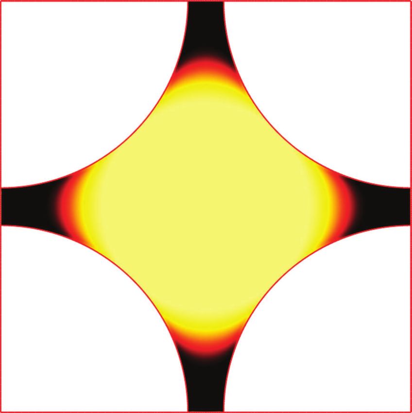
A. Žák et al. / Commun. Comput. Phys., 24 (2018), pp. 557-575                         559

lead to a lower ability of such models to fully capture soil freezing-thawing dynamics that
might occur under different general conditions. A departure from the micromechanical
considerations can be found in constitutive models of the frost heave [14, 15]. Early at-
tempts to provide more complex models for freezing soils have shortcomings such as the
absence of thawing as the reverse process [16], the incorporation of nonlinear variational
approach into thermodynamics of soil freezing [17], or the fact that they were derived by
control-volume balances rather than a fundamental thermodynamic approach [18]. As
a result, there is currently no appropriate complete macroscopic model of such complex
behavior of the soil materials. These shortcomings in model formulations can arise from
the deliberate suppression of certain effects or incomplete knowledge of all contributing
phenomena within porous media at both micro- and macro-scale.
    In an effort to enhance the knowledge of the porous media freezing and thawing
problem, we model some commonly neglected effects in order to verify, or correct, cur-
rent modeling approaches. In order to discover the microscopic mechanical behavior
of freezing and melting porous media and to assess its contribution to the macroscopic
behavior, we have developed a micro-scale model describing the thermomechanical in-
teractions occurring within a saturated soil material undergoing liquid component phase
transition. The dynamics as incorporated allows for the volume change of the phases that
affects the geometries of the interfaces.
    In Section 2, we discuss model assumptions and summarize the basic mechanical
continuum models of single phase media. Consequently, we incorporate a heat balance
and describe the coupling of all phases and physics. The formulation of a final micro-
scale thermomechanical model of the phase-change phenomenon is presented. Section
3 contains several computational experiments that use the model to study the freezing
dynamics within a micro-scale geometry and determine temperature dependencies of
some physical properties of freezing soil useful in upscaling.

2 Micro-scale model
The composition of natural soils is usually very complicated. In order to model soil
behavior, some assumptions on the structure are made.

2.1 Structural assumptions
During the temperature shifts at the ground surface around 0◦ C, several property changes
of the upper soil layer can occur as a consequence of the phase change of water in
pores. These include both mechanical and thermal properties which can vary substan-
tially when the volume of the pore water exceeds 80 % of the soil porosity. Therefore, a
saturated soil model is a convenient simplification for describing soil freezing problems
focusing on the dynamics of force interactions. This simplification is thus adopted herein.
     When describing the problem at the microscopic level, the dimensions of pores are
not negligible with regard to the dimensions of the considered pore region; therefore, the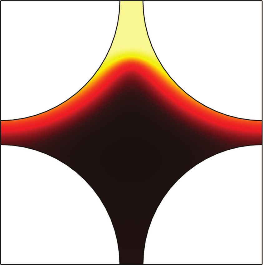
560                                         A. Žák et al. / Commun. Comput. Phys., 24 (2018), pp. 557-575

                                                          Ωi
                                  Γli
                                                         ice
                        Ωl                                            Γis
                     liquid water
                                             Γls                    Ωs

                                                               solid grain

                             Figure 1: An illustration of elementary domain Ω.

soil material has to be considered heterogeneous and consisting of clearly distinguished
and connected phases. In general, a micro-scale elementary domain∗ (MED) of freezing
saturated soil, Ω, consists of separated connected subdomains for liquid water, ice, and
soil pore skeleton along with all their mutual boundaries. A domain illustration and the
particular notation of the all domain parts are shown in Fig. 1.
    Since the motivation comes from the soil freezing phenomena, the particle and pore
sizes are considered in order of 0.1µm up to 1mm implying their surface curvatures in
orders of magnitudes between 103 and 107 m−1 . At such scales, the ratio of particle vol-
ume and particle surface becomes not-negligible, and the interface between the phases
can be characterized using the capillary theory. The Gibbs-Thomson relation then yields
depressions of the melting point of up to −1.5K for a water-ice surface.

2.2 Fluid-structure description
Focusing on the dynamics of force interactions, we now recall equations for structural be-
havior (allowing only the most important physics of the problem) using the Lagrangian
formalism. This formalism is commonly used as a standard framework for strain de-
scription of solid materials, because a difference between the initial (reference) and final
(deformed) state is subject of the interest, and thus the history of infinitesimal volumes
movement is desired. Since our concern for changes of mechanical states of the porous
media is similar, we will stay within this framework and need to relate the descriptions
of all medium components to it.
    The subdomains of Ω are occupied by the corresponding phases, which are assumed
to be continua. As the subdomains can deform by the effects of physical processes, the
∗ This term aims to characterize qualitatively rather than quantitatively a part of the considered heteroge-
neous material. For the model descriptive part, we just need to include volumes of all material’s elements,
in which the elements can be represented by their corresponding bulk properties, in the domain and do not
require any other properties of such domain so far. Naturally, assumptions on the domain can be raised as
the model has been designed for the application in an upscaling process. Then, for example, REV could be
considered.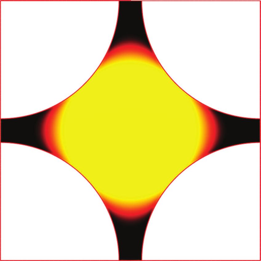
A. Žák et al. / Commun. Comput. Phys., 24 (2018), pp. 557-575                                      561

task is to characterize locally the displacement vector, u = Φ( X,t)− X, where X is the
position of an arbitrary point of a phase at the initial state and Φ( X,t) is the point’s
position at time t (the Lagrangian flow). We introduce the corresponding notations for
differential expressions: ∇ = (∂/∂X1 ,∂/∂X2 ) is the formal vector of partial derivatives in
Lagrangian coordinates, ∇ x = (∂/∂x1 ,∂/∂x2 ) is the formal vector of partial derivatives
in Eulerian coordinates, x is the Eulerian position vector, ∂/∂t( X,t) (i.e. with indication
of independent variables) is the partial derivative with respect to time in Lagrangian
coordinates, and ∂/∂t (i.e. without indication of independent variables) is the partial
derivative with respect to time in Eulerian coordinates.
    Solid parts of the MED are assumed to be (linear) elastic solid continua. We consider a
solid material marked by subscript j, j ∈{i,s}, with the initial density ̺ j , which is initially
contained in domain Ω j . The local momentum equation reads,

                    ∂vL
               ̺j       ( X,t) = ∇· P j ( X,Φ( X,t),t)+ ̺ j f ( X,t)         in Ω j , j ∈ {i,s} ,   (2.1)
                     ∂t
where vL is the Lagrangian velocity, P stands for the first Piola-Kirchhoff stress tensor,
and f is the exterior bulk force. The stress tensor can be expressed using the Cauchy
stress tensor σ as follows,

                                  P( X,Φ( X,t),t) = J F−1 σ (Φ( X,t)) ,                             (2.2)

where J = detF and F is the deformation gradient, Fmn = ∂Φ m /∂X n . Given that the
material is subjected to small deformations, the Piola-Kirchhoff stress tensor can be ap-
proximated by the Cauchy stress tensor, i.e. P ∼ = σ. As in [19], let e be the small strain
tensor,
                                          1
                                 e( u ) =    ∇u +(∇u)T ,
                                          2
then the Cauchy stress tensor can be linked to this tensor via the constitutional equation
for the linear elasticity,
                                         σ = ce,
where c is the elasticity tensor, which, for the case of an isotropic homogeneous material,
can be fully characterized by two material parameters, e.g. by Young’s modulus Ej and
by Poisson’s ratio νj . Denoting the unit tensor by I, the equation then yields,

                                    Ej                  νj Ej ∇· u j
                          σj =             e(u j )+                     I,   j ∈ {i,s} .            (2.3)
                                 (1 + νj )          (1 + νj )(1 − 2νj )

In the remaining text, we consider the aforementioned assumptions on the solid phases.
    The fluid component of the MED is assumed to act as a slightly compressible viscous
Newtonian fluid. Its strain behavior can be described using relations based on those
derived for an incompressible fluid and considering reference configuration dependency.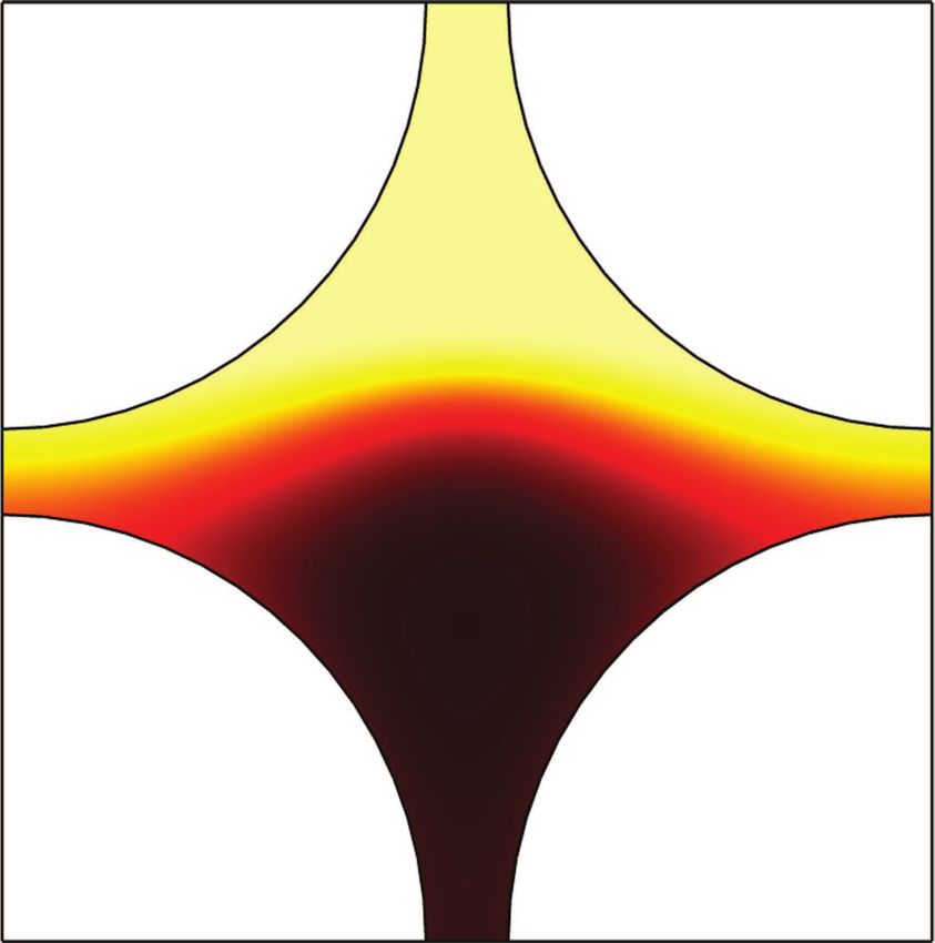
562                                          A. Žák et al. / Commun. Comput. Phys., 24 (2018), pp. 557-575

    Typically, the momentum equation of an incompressible Newtonian fluid is described
in the Eulerian coordinates by,

                                  ∂v
                             ̺l      + v ·∇ x v = ∇ x · σ l + ̺l f ,              (2.4)
                                  ∂t
where v is the Eulerian velocity, and

                                  σ l = − pI + µ ∇ x v +(∇ x v)T ,                                     (2.5)

where p is the pressure and µ is the viscosity of the fluid. Since the fluid stress tensor de-
pends on the pressure variable as well, the momentum equation must be supplemented
with an additional relation. The common choice is the continuity equation, which for an
incompressible fluid is the divergence-free vector field.
   For our purpose, the slightly compressible fluid flow can be described with the conti-
nuity equation in the form,
                                     1
                                          p +∇· u( X,t) = 0,
                                   ̺ l El
and with momentum equation (2.4) transformed into the Lagrangian coordinates (like
in [20]).
    At phase interfaces in Ω, the balance of corresponding quantities has to be considered.
They are described, in general, by the nonlinear equations coupling the state of neighbor-
ing phases (for details, see [21, 22]). In agreement with [20], the coupling of mechanical
state expresses continuity of velocity and balance of forces. At the solid-solid interface,
we consider continuity of the Lagrangian velocities, whereas at the liquid-solid interface,
we couple the fluid velocity at the deformed interface to the Lagrangian velocity with
respect to the initial (non-deformed) interface Γ(0). These conditions read as follows:

  vLs ( X,t) = vLi ( X,t)   on   Γis (0) ,    v(Φ( X,t),t) = vLj ( X,t) , j ∈ {i,s}    on    Γlj (0) . (2.6)

The balance of forces in terms of continuity of normal stresses across the deformed inter-
faces can be determined using the corresponding stress tensors which are distinctively
derived within Eulerian coordinates. To provide relations in terms of Lagrangian coordi-
nates, we transform the equations and obtain the conditions at the solid-solid interface

                 J −1 F (Ps − Pi )( X,Φ( X,t),t) n(Φ( X,t),t) = 0 on Γis (0)          (2.7)

and at the liquid-solid interface

            J −1FP j ( X,Φ( X,t),t)− σ l (Φ( X,t),t) n(Φ( X,t),t) = 0             on    Γlj (0) .      (2.8)

Here n stands for the normal vector of the interface in the Eulerian description, and j ∈
{i,s}. As conditions (2.6)-(2.8) are nonlinear and nonlocal, we apply the small-strain
assumption, and use their linearized forms, for simplicity.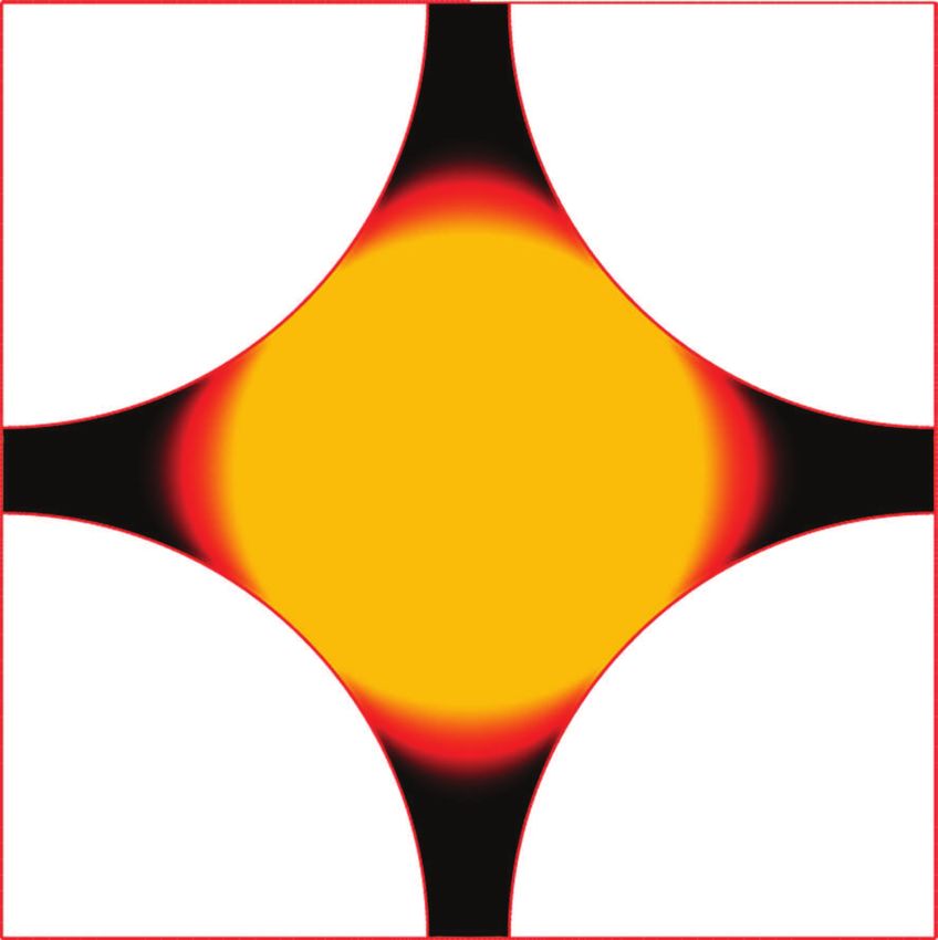
A. Žák et al. / Commun. Comput. Phys., 24 (2018), pp. 557-575                                    563

    In addition, if more interfaces intersect, another condition should be specified. For a
local equilibrium, a contact angle condition (Young’s law) may be provided

                                           γis = γls + γcosθ,                                     (2.9)

where θ is the contact angle (between liquid-ice and liquid-grain interfaces), γ, γis , and
γls are the surface energy between liquid water and ice, ice and rock skeleton, and liquid
water and rock skeleton, respectively. The contact angle characterizes the energetic influ-
ence of the rock material. However in a dynamical situation, the no-slip condition gives
arise to non-integrable flow singularities at the site of contact lines [23], indicating that
the above model approach describes the physics improperly. Thus the flow conditions at
the interface need to be reconsidered more in detail, as indicated in [24], or the flow near
the contact lines needs to be remodelled. There are several ways of relieving the singu-
larity problem including introduction of a slip law, a precursor film, or a diffuse interface
(e.g., [25–28]). In what follows, we use a diffuse interface approach.

2.3 Heat balance
Passing to the thermal behavior, we have to state heat conditions and laws within the
considered domain. Considering infinitesimal changes of the pore shape, the thermal
description can be related to the reference geometry. Here we provide the heat balance
with respect to temperature T = T ( X,t).
    Heat transport within each phase is expressed by a heat equation. Assuming a phase
with the specific heat capacity c j which is (initially) located in subdomain Ω j and which
is equipped with the instantaneous heat flux density q j , the heat equation for the phase
reads,
                      ∂T
               ̺ j c j ( X,t) = −∇·(J F−1 q j (Φ( X,t),t))    in Ω j , j ∈ {i,l,s} .     (2.10)
                      ∂t
    At the interfaces, we require continuity of the temperature and additional conditions
in terms of the heat flux. While heat fluxes can be assumed to be equal at the skeleton-
ice and skeleton-liquid interfaces, the joining of two phases of a single material must be
considered for the ice-liquid interface. According to theory, a phase transition is coupled
with the latent heat of the phase transition. Since the specific latent heat of melting of
water, lM , is very high (about 334 kJ/kg at the normal conditions), it must be included
in the heat flux balance at the interface. In contrast, the effect of the interfacial energy is
assumed to be small compared to the latent heat, [29], and can therefore be neglected in
the interfacial balance consideration. The thermal conditions then read,

                                   Ts ( X,t) = Tj ( X,t)                       on   Γ js (t) ,   (2.11)
       [qs − q j ](Φ ( X,t),t)· n (Φ( X,t),t) =0                               on   Γ js (t) ,   (2.12)
                                   Tl ( X,t) = Ti ( X,t)                       on   Γli (t) ,    (2.13)
                                                                      −1
       [qi − ql ](Φ ( X,t),t)· n (Φ( X,t),t) =̺i lM vΓ (Φ( X,t),t)J        F   on   Γli (t) ,    (2.14)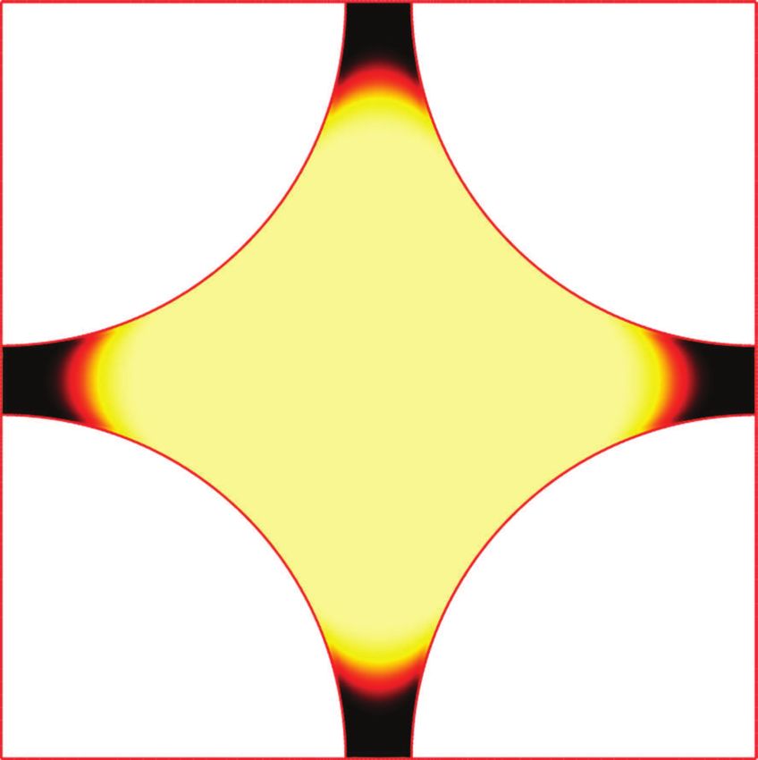
564                                        A. Žák et al. / Commun. Comput. Phys., 24 (2018), pp. 557-575

    where vΓ denotes the difference between the present Eulerian normal velocity of the
interface and its mechanical part, and j ∈ {i,l }.
    The heat flux density q j can be given by Fourier’s law, which in Lagrangian coordi-
nates reads
                                q j = −k j ∇ x Tj = −k j ∇ Tj F−1 ,                (2.15)
where k j is thermal conductivity of the phase j.
    In dealing with the thermomechanics at the scale of the interest, one should take the
effect of interfacial curvature on the condition of local equilibrium of two phases into
consideration as well. Assuming the effect of pressure is small and so too the interfacial
entropy, the condition can be expressed by the Gibbs-Thomson equation which reads,

                                 T0 − TM ( X,t)
                        ̺ i lM                  = γκ ( X,t)      on      Γli (t) ,                 (2.16)
                                       T0

where T0 is the bulk freezing point of water, TM is the local temperature value of the ice-
liquid equilibrium, γ is the surface energy of water, and κ is the curvature of the interface.

2.4 Interface model
Although the sharp interface physical model we have established above simplifies the
nonlinearities by assuming only linear relations, this may be an improper approach in
situations where the phase interface in the pore geometry is defined by temperature.
While an isothermal movement of an interface within the purely mechanical approach
represents a position change of the material points of the reference interface, (allowing
for thermal dependencies) the situation is different in the case of the two phase inter-
face of a single material. Since the liquid-ice interface is specified by the characteristic
temperature of the local phase equilibrium, its deformation is defined by the develop-
ment of the temperature field. Thus, the assumption of the linear deformation of the
interface does not need to be necessarily correct. Another shortcoming, considering the
Lagrangian framework, could be that such an interface represents a source object for the
material points within the subdomain. To avoid these difficulties, we adopt an united
description of the pore phases considering the two corresponding subdomains as one.
We can create such unified description of the pore subdomain by defining a function φ
that locally indicate the phase.
    The simplest expression of the phase indication function can be obtained using the
Heaviside step function ϑ as follows,

                                   φ( X,t) = ϑ ( TM ( X )− T ( X,t)) .                             (2.17)

The above function assigns 1 for the frozen phase (T ≤ TM ) and 0 for the melted phase
(T > TM ). Although such a definition is quite intuitive and natural, it introduces singulari-
ties with respect to the terms containing the phase-dependent quantities of the governing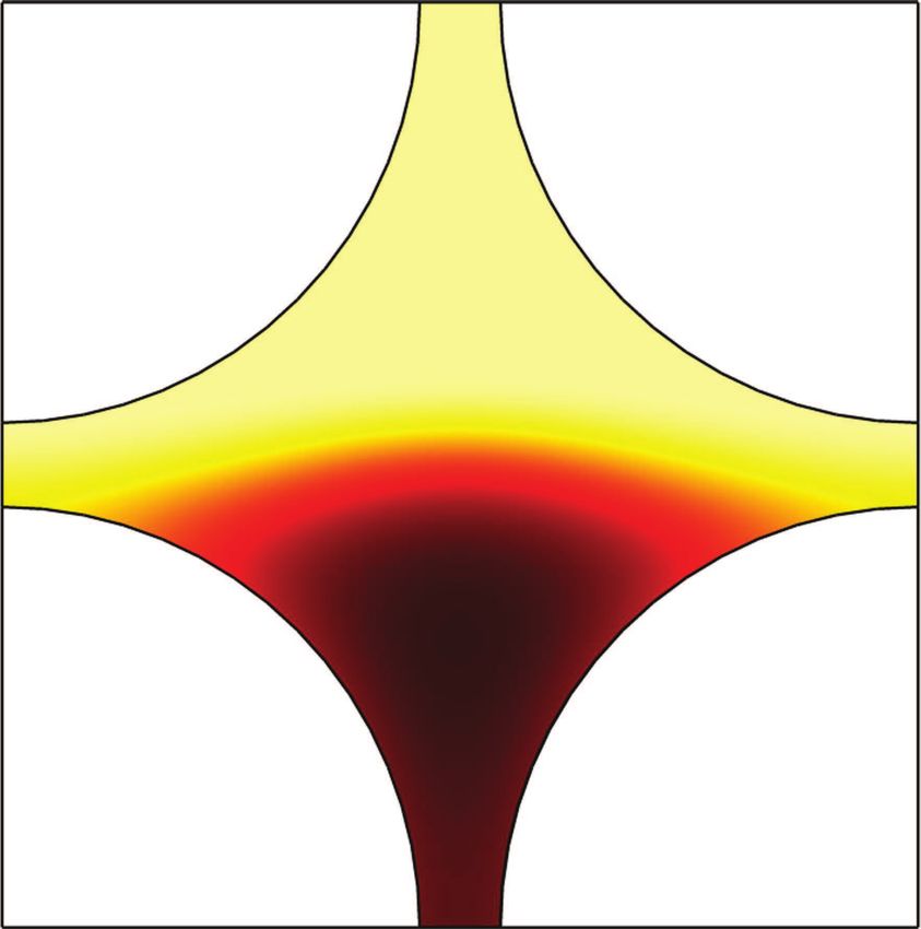
A. Žák et al. / Commun. Comput. Phys., 24 (2018), pp. 557-575                           565

laws. The problem description involving (2.17) would thus require an additional math-
ematical treatment, like in [30], and increased numerical realization demand. Therefore,
for convenience, we use a regularized form of the Heaviside step function in the phase
function definition, i.e.,
                                   φ( X,t) = ϑǫ ( TM ( X )− T ( X,t)) .                (2.18)

The regularization ϑǫ is carried out by smoothing the transition of the original Heaviside
function within the interval (−ǫ,ǫ). Convergence of the partial problem involving the
regularization using a similar smooth field has been shown in [30]. This definition allows
us to formulate the model equations in the classical way and to meet better computational
constraints.
     Full thermomechanical description of the investigated phenomenon requires deter-
mination of the liquid-ice interface. This would generally require another dynamic law
to provide the local equilibrium interface within the pore domain and to indicate the
parts of domain occupied by corresponding phases. The sharp-interface and diffuse-
interface methods (like the phase-field method or level-set method) have been widely
used in modeling of phase-transition phenomena, mostly under conditions assuming
constant specific volumes or limited structural variability. In our case both energy and
mechanical balance are crucial, and incorporation of another dynamic law would further
increase computational complexity. The diffused-interface models have been analyzed
and frequently used in the context of the interface tracking problems (see [31–35]).
     In order to avoid such difficulties, we simplify the model and assume that pore and
grain geometry is symmetric. Then we take advantage of this symmetry and estimate
the value of the interface curvature at each position in the pore in advance as described
below.
     Assuming symmetrical configuration of grains of equal size within the two-dimen-
sional domain and the perfect wetting property of the grain material when a water-ice
interface meets the grain surface (although the corresponding generalization for the hy-
drofilic property can be made), we can explore features of envelope surfaces (curves in
2D — see [36, 37]) and approximate the shape of ice phase growing from the center of the
pore subdomain by a circular pattern before it reaches the grain boundaries and by the
pattern given by the envelope curves when the phase interface becomes tangent to grains
after arriving into narrower parts of the pore.
     First the function r( X ) is determined at each point of the pore as follows. For X ∈ B0
(circle with a radius given as the distance of grains to the center of geometry M0 ), r( X )
is the radius of B0 . For X in the pore complement of B0 , r( X ) is the radius of the en-
velope circle determined as in Fig. 2 by solving a system of quadratic equations aris-
ing from geometric considerations. Then, the curvature is pre-calculated by the formula
κ ( X )= 1/r( X ). The particular melting temperature distribution in the pore can be prede-
termined using the Gibbs-Thomson equation (2.16). Eventually this approach allows to
use an expected distribution of TM ( X ) in calculation of phase-indication function (2.18).
566 A. Žák et al. / Commun. Comput. Phys., 24 (2018), pp. 557-575
O XC TC C
X
T
XM
T′
M
Figure 2: Scheme of symmetric geometrical (with axis of symmetry MO) configuration of grains (circles with
black boundary and centers C) surrounded by ice and liquid water after the ice phase reached the grain surface.
The water-ice interface going through an arbitrary point X of the pore meniscus is approximated by (red)
envelope curve TXT′ which is presented by an arc that is convex when seeing as a part of the ice phase
boundary. The point X can be associated with the radius r ( X ) of the circle (with gray boundary and center
M) corresponding to the arc. Size of the radius can be obtained from consideration of the equilibrium value of
contact angle at triple point T and of geometrical properties of triangles COM and XXM M.
2.5 Formulation of mathematical model
Denoting the pore domain by Ω p = Ωl ∪ Γli ∪ Ωi , the common heat balance law in the pore
domain reads,
∂Tp ∂φ
̺c ( X,t)+ ̺i lM ( X,t) = ∇· k∇ Tp ( X,t) in Ωp , (2.19)
∂t ∂t
where temperature Tp is naturally taken as,
Tl
in Ωl ,
Tp = TM on Γli , (2.20)
T
i in Ωi ,
and ̺, c, and k here represent effective values of the density, the specific heat capacity,
and the thermal conductivity of the material within the pore, respectively. The effective
values develop with regard to the current phase content and can be described with the
aid of the phase-indication function as well. They read,
̺ = φ̺i +(1 − φ)̺l , c = φci +(1 − φ)cl , k = φki +(1 − φ)kl .
Using this approach, we overcome the problem of variability of the phase volume by
making the interface thermally defined within the pore subdomain.A. Žák et al. / Commun. Comput. Phys., 24 (2018), pp. 557-575 567
Due to this approach, we can also provide unified laws of the structural description.
The Navier equation that holds in the pore domain is expressed in form,
∂2 u p
̺ ( X,t) = ∇· σ ( X,t) in Ωp , (2.21)
∂t2
where σ is the effective value of the stress tensor and is given as,
β i Ei
σ = φσ i +(1 − φ)σ l + φξ , ξ= I. (2.22)
1 − 2νi
Tensors σ i and σ l stand for the stress tensor of ice ((2.3) for j = i) and liquid water (2.5),
respectively. Tensor ξ represents, in the Lagrangian framework, the additional stresses
in ice that mimic the structural change during the phase transition. This tensor can be
characterized by β i , the volume expansion ratio of ice.
Now we are able to state the mathematical formulation of the considered problem of
freezing dynamics of porous media at the micro-scale level.
Consider time interval I = (0,tfinal ) and space domain Ω with its corresponding sub-
division (see Fig. 1) and with a specific symmetry allowing to have a distribution of cur-
vatures of phase interfaces in the form of a function κ ( X ) as described in Section 2.4.
The governing system for unknown functions T,u: I × Ω → R, where the functions are
naturally (with regard to the assumptions) composed as,
Ts in Ωs ∪ Γis ∪ Γls , us in Ωs ∪ Γis ∪ Γls ,
T= u= (2.23)
Tp in Ωl ∪ Ωi ∪ Γli , u p in Ωl ∪ Ωi ∪ Γli ,
reads (for t > 0) as,
∂Tp ∂φ
̺c ( X,t)+ ̺i lM ( X,t) = ∇·(k∇ Tp ( X,t)) in Ωp , (2.24)
∂t ∂t
∂2 u p
̺ 2 ( X,t) = ∇· σ ( X,t) in Ωp , (2.25)
∂t
p
+∇· u p ( X,t) = 0 in Ωp , (2.26)
̺ l El
∂Ts
̺s cs ( X,t) = ∇·(ks ∇ Ts ( X,t)) in Ωs , (2.27)
∂t
∂2 u s
̺s 2 ( X,t) = ∇· σ s ( X,t) in Ωs , (2.28)
∂t
Ts ( X,t) = Tp ( X,t) , us ( X,t) = u p ( X,t) on Γis ∪ Γls , (2.29)
ks ∇ Ts ( X,t)· n = k∇ Tp ( X,t)· n, σ s ( X,t)· n = σ ( X,t)· n on Γis ∪ Γls , (2.30)
T0 − TM ( X )
̺ i lM = γκ ( X ) in Ωp . (2.31)
T0
Specifying the domain geometry and supplementing the previous relations with ap-
propriate boundary conditions and an initial condition, we get the final mathematical568 A. Žák et al. / Commun. Comput. Phys., 24 (2018), pp. 557-575
model that can be used to give some information on soil freezing-thawing dynamics for
specific scenarios. The particular setup of considered domains and boundary and initial
conditions will be discussed in the following section in the context of the corresponding
computational results.
3 Computational results
The model described in the previous sections allows qualitative and quantitative infor-
mation on thermomechanical phenomena to be obtained for the freezing of pore water in
saturated soils at the scale determined in Section 2.1. Here we present several computa-
tional results which demonstrate thermomechanical behavior of the saturated grain-pore
structure under freezing.
The considered computational domain is square-shaped with the side length of 6.6µm
and is described in more detail in the further text. This particular geometry is illustrated
in Fig. 3(a) having its dimensions and corresponding temperature equilibrium distribu-
tion depicted in Fig. 3(b).
The mentioned computations were obtained numerically by means of the finite-
element code implemented in the environment of Comsol Multiphysics 3.5a [38]. All re-
sults below were computed using the triangular Lagrangian quadratic elements of max-
imal size of 0.05µm within the pore subdomain and solving 75570 degrees of freedom
within one symmetric half of the considered domain. The time evolution was governed
by the BDF solver with adaptive time stepping using the maximal step size of 10−4 s.
3.1 Vertical freezing
In order to provide some information on the microscopic freezing dynamics within an
upper soil layer subjected to constant cooling ambient conditions, we have performed
simulations under the following scenario.
The modeled scenario represents a vertical cross-section within a small region of the
soil material with an ideal (symmetrical) geometry and realistic physical dimensions and
properties. Its geometry is comprised of a group of four disjoint regions which represent
the soil grains and a region denoting the pore water filled pore. The particle grid is fixed
at the grain centers and the grains are allowed to deform (within the domain). The pore
content can move within the domain. The entire sample domain is subjected to a vertical
thermal gradient induced by heat flux q given on the top sample boundary. The bound-
ary and initial conditions for this particular scenario are listed in Table 1 with the notation
depicted in Fig. 3(a). The values of parameters used in simulations are presented in Ta-
ble 2. The considered configuration of porous medium sample induces the distribution
of the local equilibrium temperature as shown in Fig. 3(b).
In order to stress the importance of taking the shape of the geometry at the micro-scale
into account, this scenario has also been compared with a situation where, irrespective of
the geometry, the traditional macro-scale assumption of a constant freezing point valueA. Žák et al. / Commun. Comput. Phys., 24 (2018), pp. 557-575 569
Γt
Γ ps
Ωp
h
Ωs r
Γs Γs
Γb
(a) (b)
Figure 3: (a) Illustration and notation of the considered computational domain. Γ b , Γ s , and Γ t denote the
bottom, side, and top part of the sample outer boundary, respectively. The particular settings on these boundaries
are stated in Table 1. (b) Local equilibrium temperature distribution generated for the case of the perfect wetting
(θ = 0) for simplicity. Colors stand for the local equilibrium temperature (in [◦ C]) in the pore (size in [m]) induced
by the Gibbs-Thomson law.
Table 1: Boundary and initial conditions for geometry in Fig. 3(a). Here n stands for the outward normal vector,
q is the heat flux.
Variable Boundary Γt Boundary Γs Boundary Γb Domain Ω
u1 (σ (u)· n)1 = 0 u1 = 0 (σ (u)· n)1 = 0 u1 |t=0 = ∂u1 /∂t|t=0 = 0
u2 u2 = 0 (σ (u)· n)2 = 0 u2 = 0 u2 |t=0 = ∂u2 /∂t|t=0 = 0
T k∇ T · n = q k∇ T · n = 0 k∇ T · n = 0 T |t=0 = ∂T/∂t|t=0 = 0
Table 2: Simulation settings.
Symbol Value Symbol Value Symbol Value
cl 4.2 [kJ/(kg·K)] ci 2.1 [kJ/(kg·K)] cs 1 [kJ/(kg·K)]
ǫ 0.05 [1] El 5.33 [GPa] Ei 7.8 [GPa]
Es 75 [GPa] h 0.6 [µm] kl 0.6 [W/(m·K)]
ki 2.18 [W/(m·K)] ks 2 [W/(m·K)] lM 334 [kJ/kg]
µ 180 [Pa·s] νi 0.33 [1] νs 0.33 [1]
q 100 [W/m] r 3 [µm] ̺l 1000 [kg·m−3 ]
̺i 920 [kg·m−3 ] ̺s 2500 [kg·m−3 ] ξ 0.13 [GPa]
(γ = 0 in condition (2.16)) within the pore is used. The comparison of the freezing dynam-
ics obtained by the model (2.24)-(2.31) for the both cases is provided by Fig. 4, in which
constant freezing temperature results are on the left and the scenario results are on the570 A. Žák et al. / Commun. Comput. Phys., 24 (2018), pp. 557-575
(a) initial condition and color scale (e) t = 3.5[s]
(b) t = 0.5[s] (f) t = 4.5[s]
(c) t = 1.5[s] (g) t = 5.5[s]
(d) t = 2.5[s] (h) t = 6.5[s]
Figure 4: Comparison of the freezing dynamics. Color denotes the phases - light stands for ice phase and dark
for liquid water; remaining colors signify the diffused interface. At each time snapshot the left image is the
result for the constant equilibrium temperature (TM = −0.08[ ◦ C]). The image on the right is the result for the
equilibrium temperature distribution obtained by involving the Gibbs-Thomson relation (Fig. 3(b)).
right. The left series depicts intuitive simple dynamics in which the freezing front moves
downward following the temperature gradient as the sample cools. The pore geometry
influences the phase and temperature pattern by different thermal capacities and con-A. Žák et al. / Commun. Comput. Phys., 24 (2018), pp. 557-575 571
Figure 5: Comparison of the freezing dynamics in terms of the pore volume change. Red dashed curve stands
for the constant freezing point assumption in the pore, and blue solid curve stands for the freezing temperature
reflecting the Gibbs-Thomson law.
ductivities only. The frozen area spreads out progressively from the upper cooler parts
of the pore domain towards the bottom warmer parts following preferentially the heat
pathways which are created under the specific thermo-geometric setting. However, the
right series shows that ice begins to appear in the circular area with the lowest boundary
curvature after the sample has been supercooled and then spreads into the pore menisci
as cooling continues. This dynamics shows that the interface curvature influence pre-
dominates the influence of the temperature gradient induced by cooling. The difference
can also be seen in the progress of the pore deformation. As shown in Fig. 5, the pore vol-
ume change is approximately linear in the case of the constant freezing point (red dashed
curve) and nonlinear in the case of pore geometry induced freezing temperature (blue
solid curve). The influence of geometry causes an abrupt change to a larger deforma-
tion after the pore is sufficiently supercooled and the ice begins to become present. This
change is then followed by a small and gentle change to the final deformed state.
3.2 Parametric study
The model further enables the force action exerted on the grain boundary during the
freezing process to be evaluated. This is depicted in Fig. 6 in terms of the vertical compo-
nent of the resultant force applied by the freezing pore content along the visible bound-
ary of the upper left grain particle.
We also show the dependency of the calculated solutions on regularization parame-
ter ǫ of the pore phase coupling (2.18). Lowering the overlap width of the various phase
models (i.e. decreasing the value of ǫ) produces sharper solutions in both shapes of the
temporal quantities and changes of characteristic course of the freezing evolution. The
latter property thus causes a slightly earlier initiation of the changes. This is due to the
reduced effect of averaged behavior on the diffused interface. These results were pro-
duced for the setting described in Table 2 and with the values of ǫ in Fig. 6 and the same
conditions as in Table 1.572 A. Žák et al. / Commun. Comput. Phys., 24 (2018), pp. 557-575
Figure 6: Study of the model behavior with respect to parameter ǫ. The study is presented in terms of the
vertical component of resultant force applied by the freezing pore content along the visible boundary part of the
upper left grain particle. The results are plotted for ǫ = 0.03 (red line), 0.05 (orange dashed line), 0.075 (green
dash-dot line), and 0.1 (blue dotted line).
3.3 Averaging mean values
The model can be also used to determine temperature dependencies of the material prop-
erties of the soil which can be used for future upscaling investigations. Since differences
in the temperature within such a tiny domain at one moment are small (∝ 10−5 ), the
mean value of the temperature over the whole domain can be considered as a variable
describing the state of the investigated volume Ω, and the mean values of the material
parameters can therefore be related to this state quantity. The particular relations com-
puted for the same setting (see Tables 1 and 2) as in the previous case are depicted in
Fig. 7.
4 Conclusion
The model presented in the paper was created using natural multi-phase and multi-
physics coupling of classical single-phase and single-physics continuum models. The
model conceptualization allows for the simulation of the dynamics of the thermomechan-
ical interaction during phase transitions at the microscopic scale that was considered, as
well as generation of information on the distinctive properties and on structural changes
during phase transition. The model is intended to provide preliminary results in an effort
to broaden the knowledge of freezing and thawing processes in porous media. Therefore,
the current scope of the model — two-dimensional symmetric scenarios — is planned to
be generalized and extended to include other phenomena.
The current model indicates key factors such as: non-trivial thermodynamics of fluid-
structure interaction during the phase transition influenced by curved grain geometry, or
characteristic courses of the force action exerted on grains within a single pore that might
be confronted by some macro-scale modeling approaches. The article also indicated howA. Žák et al. / Commun. Comput. Phys., 24 (2018), pp. 557-575 573
Figure 7: The mean values of some material properties as functions of the temperature.
the obtained computational results can be averaged in order to provide a suitable infor-
mation for larger, practical scales.
Acknowledgments
Partial support of the project of Czech Ministry of Education, Youth and Sports [Kontakt
II LH14003, 2014-2016]; the project of the Czech Science Foundation [No. 17-06759S]; and
of the project of the Student Grant Agency of the Czech Technical University in Prague
[No. SGS14/206/OHK4/3T/14 2014-2016].
References
[1] G. Beskow, Soil freezing and frost heaving with special application to roads and railroads,
Reprinted 1991 CRREL Spec. Rep. 91-23: The Swedish Geological Society, C, no. 375, Year
Book no.3 (Translated by J.O. Osterberg), 1935.
[2] G. L. Guyman, R. L. Berg and T. V. Hromadka, Mathematical model of frost heave and thaw
settlement in pavements, CRREL Report 92-2, U.S. ACoE, Cold Regions Res. and Eng. Lab.,
1993.
[3] L.-C. Lundin, Water and heat flows in frozen soils. Basic theory and operational modeling,
Ph.D. thesis. Uppsala University, Uppsala, Sweden, 1989.574 A. Žák et al. / Commun. Comput. Phys., 24 (2018), pp. 557-575
[4] M. Furuzumi, Y. Takeshita, M. Kurashige, F. Nishimura, K. Hirose and K. Imai, Thermal and
freezing strains on a face of wet sandstone samples under a subzero temperature cycle, J.
Therm. Stresses, 27 (2004), 331–344.
[5] J. Abraham, Methane release from melting permafrost could trigger dangerous global
warming, The Guardian, October 13, 2015.
[6] J. Li, Y. Luo, S. Natali, E. Schuur, J. Xia, E. Kowacyk and Y. Wang, Modeling permafrost thaw
and ecosystem carbon cycle under annual and seasonal warming at an Arctic tundra site in
Alaska, J. Geophys. Res.: Biogeosciences, 119/6 (2014), 1129–1146.
[7] K. Hansson, J. Šimůnek, M. Mizoguchi, L.-C. Lundin and M. Th. van Genuchtenet, Water
flow and heat transport in frozen soil: Numerical solution and freeze-thaw applications,
Vadose Zone J., 3 (2004), 693–704.
[8] D. J. Nicolsky, V. E. Romanovsky and G. G. Panteleev, Estimation of soil thermal properties
using in-situ temperature measurements in the active layer and permafrost, Cold Reg. Sci.
Technol., 55 (2009), 120–129.
[9] R. D. Miller, Frost heaving in non-colloidal soils, Proc. 3rd Int. Conference on Permafrost,
Edmonton, Canada, (1978), 707–713.
[10] R. R. Gilpin, A Model for the prediction of ice lensing and frost heave in soils, Water Resour.
Res., 16/5 (1980), 918–930.
[11] A. W. Rempel, Microscopic and environmental controls on the spacing and thickness of
segregated ice lenses, Quaternary Res., 75 (2011), 316–324.
[12] S. Taber, The mechanics of frost heaving, J. Geol., 38 (1930), 303–317.
[13] A. W. Rempel, J. S Wettlaufer and M. G Worster, Premelting dynamics in a continuum model
of frost heave, J. Fluid Mech., 498 (2004), 227–244.
[14] D. Blanchard and M. Frémond, Soil frost heaving and thaw settlement, Proc. 4th Int. Symp.
on Ground Freezing Rotterdam, Netherlands, 1985.
[15] R. L. Michalowski, A Constitutive model of saturated soils for frost heave simulations, Cold
Reg. Sci. Technol., 22/1 (1993), 47–63.
[16] O. Coussy, Poromechanics of freezing materials, J. Mech. Phys. Solids, 53 (2005), 1689–1718.
[17] J. Hartikainen and M. Mikkola, Thermomechanical model of freezing soil by use of the the-
ory of mixtures, Proc. of the 6th Finnish Mechanics Days, Oulu, Finland, 1997, 1–6.
[18] N. Li, F. Chen, B. Xu and G. Swoboda, Theoretical modeling framework for an unsaturated
freezing soil, Cold Reg. Sci. Technol., 54 (2008), 19–35.
[19] M. Brdička, B. Sopko and L. Samek, Continuum Mechanics, Academia, Prague, 2000 (in
Czech).
[20] A. Mikelić and M. F. Wheeler, On the interface law between a deformable porous medium
containing a viscous fluid and an elastic body, Math. Mod. Meth. Appl. S., 22 (2012), 1–32.
[21] M. E. Gurtin and I. Murdoch, A Continuum Theory of Elastic Material Surfaces, Arch. Ra-
tional Mech. Anal., 57 (1975), 291–323.
[22] M. E. Gurtin and A. Struthers, Multiphase Thermomechanics with Interfacial Structure.
3. Evolving Phase Boundaries in the Presence of Bulk Deformation, Arch. Rational Mech.
Anal., 112 (1990), 97–160.
[23] S. Davis, Interfacial fluid dynamics, In: G. Batchelor, H. Moffatt, M. Worster , editors. Per-
spectives in Fluid Dynamics, Cambridge University Press, 2002.
[24] M. G. Worster, Solidification of Fluids, In: G. Batchelor, H. Moffatt, M. Worster , editors.
Perspectives in Fluid Dynamics, Cambridge University Press, 2002.
[25] P. de Gennes, Wetting: statics and dynamics, Rev. Mod. Phys., 57 (1985), 827–863.
[26] D. M. Anderson, G. B. McFadden and A. A. Wheeler, Diffuse-Interface Methods in FluidA. Žák et al. / Commun. Comput. Phys., 24 (2018), pp. 557-575 575
Mechanics, NIST Report 6018, 1997.
[27] P. Yue, J. J. Feng, C. Liu and J. Shen, A diffuse-interface method for simulating two-phase
flows of complex fluids, J. Fluid Mech., 515 (2004), 293–317.
[28] K. E. Teigen, P. Song, J. Lowengrub and A. Voigt, A diffuse-interface method for two-phase
flows with soluble surfactants, J. Comput. Phys., 230/2 (2011), 375–393.
[29] M. E. Gurtin, On the two-phase Stefan problem with interfacial energy and entropy, Arch.
Ration. Mech. An., 96/3 (1986), 199–241.
[30] A. Žák, M. Beneš and T. H. Illangasekare, Analysis of model of soil freezing and thawing,
IAENG International Journal of Applied Mathematics, 43/3 (2013), 127–134.
[31] G. Caginalp, An Analysis of a Phase Field Model of a Free Boundary, Arch. Rational Mech.
Anal., 92 (1986), 205–245.
[32] A. A. Wheeler, B. T. Murray and R. J. Schaefer, Computation of Dendrites using a Phase Field
Model, Physica D, 66 (1993), 243–262.
[33] C. M. Elliott, M. Paolini and R. Schätzle, Interface Estimates for the Fully Anisotropic Allen-
Cahn Equation and Anisotropic Mean Curvature Flow, Math. Models Methods Appl. Sci.,
6 (1996), 1103–1118.
[34] M. Beneš, Diffuse-Interface Treatment of the Anisotropic Mean-Curvature Flow, Applica-
tions of Mathematics, 48/6 (2003), 437–453.
[35] H. Abels, H. Garcke and G. Grün, Thermodynamically Consistent, Frame Indifferent Dif-
fuse Interface Models for Incompressible Two-Phase Flows with Different Densities, Math.
Models Methods Appl. Sci., 22/3 (2012), 40pp.
[36] N. Kruithof and G. Vegter, Envelope Surfaces, Proc. 26th Annual Symp. on Comp. Geometry
(SCG ’06), Sedona, Arizona, USA, (2006), 411–420.
[37] D. Velichová, Constructive Geometry, electronic book, Department of Mathematics, Faculty
of Civil Engineering, Slovak Technical University, Bratislava, 2003.
[38] https://www.comsol.comYou can also read